New robust estimators for the fixed effects negative binomial model: a simulation and real-world applications to European panel data

This study introduces a more flexible approach by employing the fixed effects negative binomial model to address challenges associated with outliers and dispersion. Unlike previous studies that focused on the robust estimation of the Poisson model with fixed effects, which assumes equidispersion and cannot handle dispersion in count panel data, we develop novel estimators specifically designed for the fixed effects negative binomial panel regression model in the presence of outliers, under-dispersion, and over-dispersion. The methodology is assessed through comprehensive simulation experiments across different scenarios. A comprehensive empirical analysis is conducted using updated and extended panel datasets on COVID-19 and patent applications in Europe. The results of both Monte Carlo simulation and the empirical studies indicate that the robust estimators: the robust fixed negative binomial Huber, fixed negative binomial Hampel, and fixed negative binomial Tukey estimators, outperform the classical non-robust fixed negative binomial estimator.

1 Introduction

The negative binomial (NB) regression model has become a widely utilized tool in panel data analysis across various fields, including economics, healthcare, demography, and environmental sciences (see Ahmed et al. [1], Abonazel et al. [2], and Youssef et al. [3]). Panel data analysis has emerged as a prominent area of research in econometrics literature as it involves studying data along both the temporal and sectoral dimensions to derive the maximum benefit from the available data. Panel datasets combine cross-sectional and time-series observations, enabling a more in-depth analysis of the data over time [4, 5]. By including individual-specific fixed effects, panel data can account for these differences and provide more accurate estimates of the effects of the variables of interest. Within this framework, count panel data models are particularly relevant when the dependent variable represents non-negative integer values generated from counting the occurrence of a particular event, for example, the number of accidents on roads, patents granted to countries and companies, and the number of deaths due to a specific disease (see Winkelmann [6]).

One of the key challenges in analyzing count panel data is the issue of over-dispersion; this problem appears when the variance of the dependent variable is greater than the mean. Therefore, the NB panel model has a dispersion parameter ϕ_i; this parameter allows var(y_it) > E(y_it). This violates the core assumption of the classical Poisson model and often leads to inefficient or biased estimates. To address this limitation, the NB model is a powerful statistical model that is commonly used in analyzing count data. Unlike the Poisson model, the NB model is capable of handling over-dispersion in count panel data; this characteristic makes it an important model in various fields, such as economics, finance, public health, criminology, environmental health, transportation, finance, and law, where it provides a more flexible and accurate approach for analyzing count data. Therefore, several studies have focused on the use of the NB model. For example, Cameron and Trivedi [7], Yaacob et al. [8], Hana [9], Al-Taweel and Algamal [10], Alobaidi et al. [11], Rashad et al. [12], Niang et al. [13], Liu et al. [14], and Suryadi et al. [15].

Therefore, the FENB model is great importance in statistical analysis due to its ability to address over-dispersion in count panel data and control unobserved heterogeneity among individuals or entities in panel data. The model captures individual-specific or entity-specific characteristics that are constant over time. The FENB model finds applications in various fields such as economics, public health, criminology, and social sciences. Youssef et al. [16] conducted a study on estimating the number of patents in some high-income countries using the NB model and Poisson model based on the panel data models. The research aimed to develop accurate models for predicting patents. The results indicate that the FENB model is more suitable and performs better in analyzing the data. This research offers valuable contributions to the field of patent analysis by providing reliable models for estimating patents, enhancing our understanding of the factors that influence global patent trends, and providing useful insights for researchers and policymakers in the field of estimating patents. Kumara and Chin [17] conducted a study analyzing accident data for 41 countries over 15 years. They used the FENB model to examine the effect of socioeconomic and infrastructure factors on fatal road accidents in the Asia-Pacific region. The study also employed the AIC statistic to assess the suitability of the model. Guimaraes [18] used the FENB model under a specific set of assumptions. The study showed that this model effectively addresses over-dispersion. This research emphasizes the significance of the FENB model for accurately analyzing count panel data, particularly in the presence of over-dispersion. In the FENB model, Hausman et al. [19] added the individual fixed effects α_i and the NB dispersion parameter (ϕ_i) into the model. Then, the FENB model given is

$\begin{array}{l}f(y_{it}|{\theta }_i)=\frac{\Gamma ({\lambda }_{it}+y_{it})}{\Gamma ({\lambda }_{it})\Gamma (y_{it}+1)}{\left(\frac{1}{1+{\theta }_i}\right)}^{{\lambda }_{it}}{\left(\frac{{\theta }_i}{1+{\theta }_i}\right)}^{y_{it}},\\ i=1,2,\dots ,N;t=1,2,\dots ,T,& (1)\end{array}$

where y_it is the dependent variable and takes values of non-negative integers, i.e., y_it ≥ 0. The mean and the variance of the NB model with fixed effects are not equal. Γ(·) is the gamma function, and ${\theta }_i=\frac{{\alpha }_i}{{\varphi }_i}$ is the parameter of the individual effects and dispersion, which is assumed to be constant over time for each cross section, while λ_it depends on covariates by the function $ln({\lambda }_{it})=X_{k,it}^{\prime }\beta$.

We can use the conditional maximum likelihood (CML) estimation method to estimate the parameters of the FENB model [19]. The NB model with fixed effects assumes that for a given cross section (i), the dependent variable (y_it) is independent over time and $\sum _{t=1}^T{y}_{it}$ has a NB distribution with parameters θ_i and $\sum _{t=1}^T{\lambda }_{it}$, where

${\displaystyle \sum _{t=1}^T}{y}_{it}~\text{NB}\left[{\theta }_i{\displaystyle \sum _{t=1}^T}{\lambda }_{it},\left({\theta }_i{\displaystyle \sum _{t=1}^T}{\lambda }_{it}\right)(1+{\theta }_i)\right].$

For an individual (i), the dependent variable y_it is independent over time as follows:

$\begin{array}{l}f\left({\displaystyle \sum _{t=1}^T}{y}_{it}\right)=\left[\frac{\Gamma \left({\displaystyle {\sum }_{t=1}^T}{\lambda }_{it}+{\displaystyle {\sum }_{t=1}^T}{y}_{it}\right)}{\Gamma \left({\displaystyle {\sum }_{t=1}^T}{\lambda }_{it}\right)\Gamma \left({\displaystyle {\sum }_{t=1}^T}{y}_{it}+1\right)}\right]\\ \left[{\left(\frac{1}{1+{\theta }_i}\right)}^{{\displaystyle {\sum }_{t=1}^T}{\lambda }_{it}}\right]\left[{\left(\frac{{\theta }_i}{1+{\theta }_i}\right)}^{{\displaystyle {\sum }_{t=1}^T}{y}_{it}}\right].\end{array}$

The joint probability function for the i^th observation for Equation 1 is

$\begin{array}{l}f(y_{i1},\dots ,y_{iT})={\displaystyle \prod _{t=1}^T\{\left[\frac{\Gamma ({\lambda }_{it}+y_{it})}{\Gamma ({\lambda }_{it})\Gamma (y_{it}+1)}\right]}\\ \left[{\left(\frac{1}{1+{\theta }_i}\right)}^{{\lambda }_{it}}\right]\left[{\left(\frac{{\theta }_i}{1+{\theta }_i}\right)}^{y_{it}}\right]\end{array}$

Then, the conditional joint probability function for the i^th observation is

$\begin{array}{r}f(y_{i1},\dots ,y_{iT}|{\displaystyle \sum _{t=1}^T}{y}_{it})=\left[\frac{\Gamma \left({\displaystyle {\sum }_{t=1}^T}{\lambda }_{it}\right)\Gamma \left({\displaystyle {\sum }_{t=1}^T}{y}_{it}+1\right)}{\Gamma \left({\displaystyle {\sum }_{t=1}^T}{\lambda }_{it}+{\displaystyle {\sum }_{t=1}^T}{y}_{it}\right)}\right].\\ \times \left({\displaystyle \prod _{t=1}^T}\frac{\Gamma ({\lambda }_{it}+y_{it})}{\Gamma \left({\lambda }_{it}\right)\Gamma \left(y_{it}+1\right)}\right)\end{array}$

The CML estimation of the NB model with fixed effects can be obtained by maximizing the following log CML function:

$\begin{array}{l}L(y_{i1},\dots ,y_{iT}\mid {\displaystyle \sum _{t=1}^T{y}_{it}})={\displaystyle \sum _{i=1}^N\{\ln \Gamma \left({\displaystyle \sum _{t=1}^T{\lambda }_{it}}\right)+\ln \Gamma \left({\displaystyle \sum _{t=1}^T{y}_{it}}+1\right)}\\ -\ln \Gamma \left({\displaystyle \sum _{t=1}^T{\lambda }_{it}}+{\displaystyle \sum _{t=1}^T{y}_{it}}\right)+{\displaystyle \sum _{t=1}^T[\ln \Gamma ({\lambda }_{it}+y_{it})-\ln \Gamma ({\lambda }_{it})}\\ -\ln \Gamma (y_{it}+1)]\}.\end{array}$

For a more comprehensive understanding of CML estimation and its applications see Yousse et al. [16, 20]. In the context, the FENB model is particularly useful because it not only accounts for over-dispersion but also controls for unobserved, time-invariant heterogeneity among individuals. This makes the FENB model a powerful tool for analyzing panel count data with complex structures. However, one major issue that has been neglected in the literature is the effect of outliers on parameters estimation in the FENB model. Outliers can occur due to rare events or abnormal changes in specific units over time. Classical estimation techniques, such as the CML, are known to be highly sensitive to such outliers. This highlights the need for robust estimation methods that can produce accurate and stable results even in the presence of outliers. Despite the progress made in developing robust estimators for the fixed effects Poisson model by Ahmed et al. [1], Abonazel et al. [2], and Youssef et al. [3], there has been little interest in extending these robust methods to the NB model. This gap in literature provides a key motivation for the present study.

2 Robust FENB model estimates

According to the work of Youssef et al. [3], who introduced robust estimation methods for the Poisson fixed effects panel model, this study extends the robustness framework to the NB case to accommodate both under-dispersion and over-dispersion in count panel data. Accordingly, this section aims to develop robust estimators for the FENB model in the presence of dispersion and outliers, based on the Huber, Hampel, and Tukey weight functions. The performance of these estimators is evaluated through Monte Carlo simulations under varying levels of outliers, dispersion levels, cross-sectional sizes, and time dimensions. Furthermore, the proposed methods are applied to real-world datasets in two empirical applications involving selected European countries, providing strong evidence of their practical effectiveness.

The NB model addresses over-dispersion that may exist in the data, where the model provides more accurate and reliable estimates; this makes it suitable for a wide range of applications in various fields. The count panel data can contain outliers, and these outliers can have a significant impact on the estimated parameters, where some studies focus on addressing outliers in some models using different estimation methods (see for example Huber [21, 22], Rousseeuw and Leroy [23], Garay et al. [24], Toka and Cetin [25], Susanti et al. [26], Maronna et al. [27], Tüzun et al. [28], Youssef et al. [3, 29], and Ke et al. [30]). On the other hand, panel data regression models may suffer from outliers that can negatively affect classical estimation methods, where there are limited studies on robust estimation methods for fixed effects panel data regression model (see Beyaztas and Bandyopadhyay [31], Amelia et al. [32], Víšek [33], and Bramati and Croux [34]).

In this context, there is not a specific robust method available for estimating parameters in the FENB regression model. Therefore, we propose a robust estimation method for NB regression to deal with count panel data when these data contain outliers. The method utilizes robust estimation techniques that are less sensitive to the influence of outliers, providing more accurate and robust parameter estimates. These methods are based on weight functions that include Huber, Hampel, and Tukey bisquare and minimize the residuals, aiming to improve the robustness and reliability of parameter estimation in the presence of outliers, see for example Hampel et al. [35] and Venables and Ripley [36]. The residuals of the i^th observation for the FENB model can be expressed as

$R_{it}=y_{it}-\left(\frac{{\alpha }_i}{{\varphi }_i}{\displaystyle \sum _{t=1}^T}exp(X_{k,it}^{\prime }\beta )\right).$

The robust estimator for the FENB model can be obtained by minimizing the objective function (ρ) concerning all β, which can be expressed as follows:

$\begin{array}{ll}{\widehat{\beta }}_R=min{\displaystyle \sum _{i=1}^N}{\displaystyle \sum _{t=1}^T}\rho \left(\frac{{\xi }_{it}}{{\widehat{\sigma }}_{MAD}}\right),& (2)\end{array}$

where ${\xi }_{it}=\frac{R_{it}}{{\left({\widehat{\theta }}_i\sum _{t=1}^T{\lambda }_{it}\right)}^{1/2}}$, ${\lambda }_{it}=exp(X_{k,it}^{\prime }\beta )$, and ${\widehat{\sigma }}_{MAD}$ is the estimated standard deviation, where calculated using the median absolute deviation, which is defined as follows:

${\widehat{\sigma }}_{\text{MAD}}=1.4826\times Med\left(|{\xi }_{it}-Med({\xi }_{it})|\right),$

where Med is the median. Based on the function ρ(ξ_it), we can obtain the robust estimator of β by differentiating the objective function (ρ) concerning the parameters β, and equate the partial derivatives to zero in Equation 2, this yields the following expression:

$\begin{array}{ll}{\displaystyle \underset{\beta }{min}}{\displaystyle \sum _{i=1}^N}{\displaystyle \sum _{t=1}^T}\psi \left(\frac{{\xi }_{it}}{{\widehat{\sigma }}_{MAD}}\right)\frac{\partial }{\partial \beta }{\xi }_{it}=0,& (3)\end{array}$

where ψ(u_it) is called the influence function and equal ${\rho }^{\prime }(u_{it})$. We can rewrite the Equation 3 by using the weight function _ξ(u_it), which equals $\frac{\psi (u_{it})}{u_{it}}$, and then, we can obtain the first-order condition for robust estimators as follows:

$\begin{array}{ll}{\displaystyle \sum _{i=1}^N}{\displaystyle \sum _{t=1}^T}{\xi }_{it}^{\prime }{W}_{\xi }({\xi }_{it}){\xi }_{it}=0,& (4)\end{array}$

where ${\xi }_{it}^{\prime }=\frac{\partial }{\partial \beta }{\xi }_{it}$ and W_ξ(ξ_it) is matrix (NT × NT). Three robust estimates for β in the FENB model can be obtained by solving Equation 4 using the weight functions of Huber (W_HR(ξ_it)), Hampel (W_HM(ξ_it)), and Tukey bisquare (W_TK(ξ_it)), as introduced by Baltagi [37] and Youssef et al. [3] in the context of panel data.

We will present an algorithm for handling outliers in the NB panel data model with fixed effects to obtain stable and robust estimates as follows:

1. Estimate the CML estimator (${\widehat{\beta }}_{\mathrm{\text{NOFNB}}}$) using the algorithm presented by Hausman et al. [19] as an initial estimation.

2. Calculate residuals value ${\xi }_{it}=\frac{R_{it}}{{\left({\widehat{\theta }}_i\sum _{t=1}^T{\lambda }_{it}\right)}^{1/2}}$ based on the previous estimation.

3. Calculate median absolute deviation ${\widehat{\sigma }}_{\mathrm{\text{MAD}}}$.

4. Calculate standardized residuals $u_{it}=\frac{{\xi }_{it}}{{\widehat{\sigma }}_{\mathrm{\text{MAD}}}}$.

5. Calculate the values of the weight function W_ξ(ξ_it). We can use one of the three functions: W_HR(ξ_it), W_HM(ξ_it), and W_TK(ξ_it).

6. Estimate one of the three estimators (${\widehat{\beta }}_{\mathrm{\text{FNBHR}}},{\widehat{\beta }}_{\mathrm{\text{FNBHM}}},$ or ${\widehat{\beta }}_{\mathrm{\text{FNBTK}}}$) based on the weight function W_ξ(ξ_it) used in the previous step.

7. Repeat steps 2–6 to obtain the convergent estimates of ${\widehat{\beta }}_{\mathrm{\text{FNBHR}}},{\widehat{\beta }}_{\mathrm{\text{FNBHM}}},$ or ${\widehat{\beta }}_{\mathrm{\text{FNBTK}}}$ estimators.

8. Examine the significance of the explanatory variables on the response variable and compare the performance of these estimators using some criteria; for example, the Akaike information criterion (AIC) and Bayesian information criterion (BIC). The AIC and BIC are calculated as follows:

$\text{AIC}=2k-2log(likhod);\text{BIC}=klog(n)-2log(likhod),$

where k is the number of coefficients, and likhod denotes maximum likelihood values.

3 Simulation design and evaluation of estimators

In this section, we will present an algorithm to evaluate the impact of outliers on the estimates of the FENB model using a Monte Carlo simulation procedure to conduct a comprehensive analysis to understand the flexibility of the NB model with fixed effects in the presence of outliers. The simulation was conducted using R software. This algorithm was designed specifically for the Monte Carlo simulation study of the FENB model, where it aims to assess the model's sensitivity and accuracy in various conditions. The results from this simulation are expected to contribute significantly to the existing literature, offering an accurate perspective on the applicability and reliability of the FENB model in empirical research, especially in fields where extreme values are not merely outliers but pivotal points of interest. The algorithm utilized for conducting the Monte Carlo simulation study of the FENB model is as follows:

1. We can construct the panel dataset to calculate the total samples size (n) as follows:

(a) Set the dimensions for the cross-sectional size at N = 50, 100, 200, and 400 to indicate small, moderate, and large units, respectively.

(b) Set the dimensions for time-series size at T = 5, 10, and 20 to indicate various sizes for the time periods.

2. We generate the count panel dataset by following these steps:

(a) The values of true parameters for β₁, β₂, and β₃ were selected to be 1.

(b) The dispersion parameter (ϕ) was set at 1/2 and 2 to denote under-dispersion and over-dispersion, respectively.

(c) The explanatory variables $(X_{it}^k)$ were generated from a uniform distribution on the interval (−1, 1).

(d) Generate the response variable (y_it) from the NB distribution with an average ${\theta }_i\sum _{t=1}^T{\lambda }_{it}$.

(e) Set the outliers (τ%) to be 0%, 5%, 10%, 15%, and 20% of the total observations for the response variable. When the proportion of outliers is zero (τ = 0%), it indicates that the count panel dataset does not contain any outliers.

(f) Generate the outliers from NB distribution with an average $4\mathrm{\text{IQR}}\left[{\theta }_i\sum _{t=1}^T{\lambda }_{it}\right]$, where IQR is the interquartile range.

3. Estimate the non-robust estimator (${\widehat{\beta }}_{\mathrm{\text{NOFNB}}}$) of the generated FENB model.

4. Estimate the proposed robust estimators (${\widehat{\beta }}_{\mathrm{\text{FNBHR}}},{\widehat{\beta }}_{\mathrm{\text{FNBHM}}},$ or ${\widehat{\beta }}_{\mathrm{\text{FNBTK}}}$) of the generated FENB model with the following steps:

(a) Calculate residuals value ${\xi }_{it}=\frac{R_{it}}{{\left({\widehat{\theta }}_i\sum _{t=1}^T{\lambda }_{it}\right)}^{1/2}}$ based on the previous estimation.

(b) Calculate median absolute deviation ${\widehat{\sigma }}_{\mathrm{\text{MAD}}}$.

(c) Calculate standardized residuals $u_{it}=\frac{{\xi }_{it}}{{\widehat{\sigma }}_{\mathrm{\text{MAD}}}}$.

(d) Calculate the values of the three functions: W_HR(ξ_it), W_HM(ξ_it), and W_TK(ξ_it).

(e) Estimate the three robust estimators (${\widehat{\beta }}_{\mathrm{\text{FNBHR}}},{\widehat{\beta }}_{\mathrm{\text{FNBHM}}},$ and ${\widehat{\beta }}_{\mathrm{\text{FNBTK}}}$) based on the three weight functions (W_HR(ξ_it), W_HM(ξ_it), and W_TK(ξ_it)) calculated in the previous step.

(f) Repeat steps (a)–(e) to obtain the convergent estimates of ${\widehat{\beta }}_{\mathrm{\text{FNBHR}}},{\widehat{\beta }}_{\mathrm{\text{FNBHM}}},$ and ${\widehat{\beta }}_{\mathrm{\text{FNBTK}}}$ estimators.

5. For all simulation experiments, we conducted 500 replications.

6. We evaluate the performance of these estimators through the following steps:

(a) The mean squared error (MSE) and mean absolute error (MAE) are calculated for N, T, ϕ, and τ different for each parameter separately as follows:

$\text{MSE}=\frac{1}{\text{L}}{\displaystyle \sum _{l=1}^{\text{L}}}{({\widehat{\beta }}_l-\beta )}^2;\text{MAE}=\frac{1}{\text{L}}{\displaystyle \sum _{l=1}^{\text{L}}}|{\widehat{\beta }}_l-\beta |,$

where ${\widehat{\beta }}_l$ represents the estimated coefficient vector in the l^th experiment of L replicated simulations, and β denotes the true coefficient vector.

(b) The mean relative efficiency (MRE) is calculated for all T and τ for each N and ϕ separately to evaluate the efficiency of estimators (FNBHR, FNBHM, and FNBTK). The MRE is calculated using the following formula:

$\text{MRE}({\widehat{\beta }}_R)=\frac{\text{MSE}({\widehat{\beta }}_{NOFNB})}{\text{MSE}({\widehat{\beta }}_R)},$

where ${\widehat{\beta }}_R$ is ${\widehat{\beta }}_{FNBHR}$, ${\widehat{\beta }}_{FNBHM}$, and ${\widehat{\beta }}_{FNBTK}$ estimators. The best efficient estimator is the one with the highest MRE.

The simulation results are presented in Tables 1–4 for small, moderate, and large sample sizes. These tables report the total MSE and total MAE values for four estimators: the classical (non-robust) estimator NOFNB and three robust estimators (FNBHM, FNBHR, and FNBTK). The simulation is conducted under various scenarios defined by cross-sectional sizes (N = 50, 100, 200, and400), time periods (T = 5, 10, and20), outlier proportions (τ = 0%, 5%, 10%, 15%, and20%), and two dispersion levels representing under-dispersion (ϕ = 0.5) and over-dispersion (ϕ = 2).

Table 1

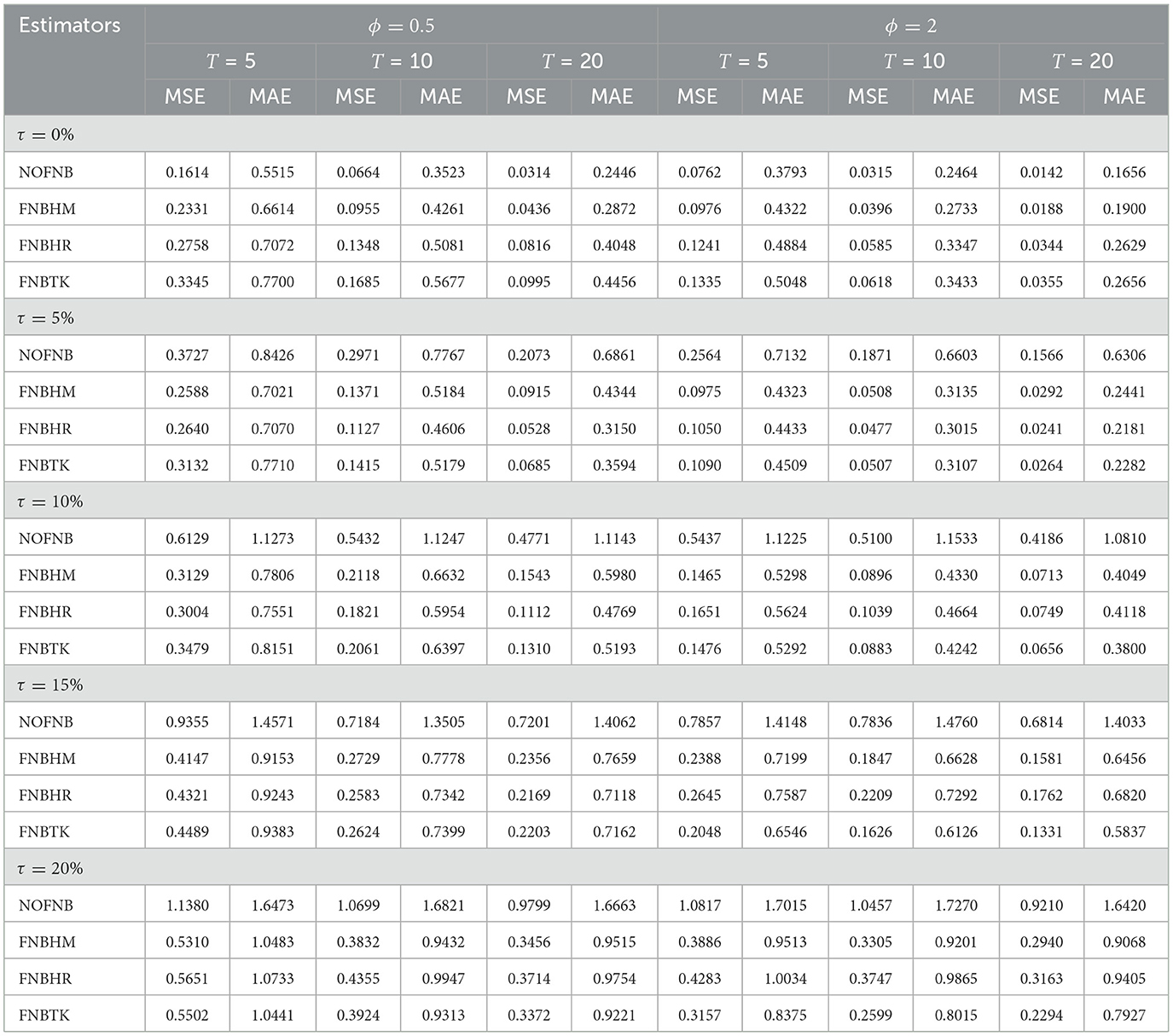
Table 1. MSE and MAE values of non-robust and robust estimates when N = 50.

Table 2

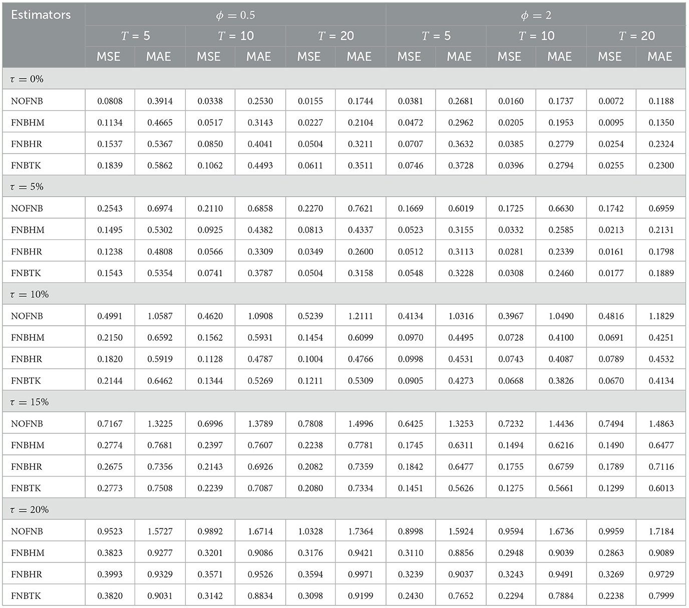
Table 2. MSE and MAE values of non-robust and robust estimates when N = 100.

Table 3

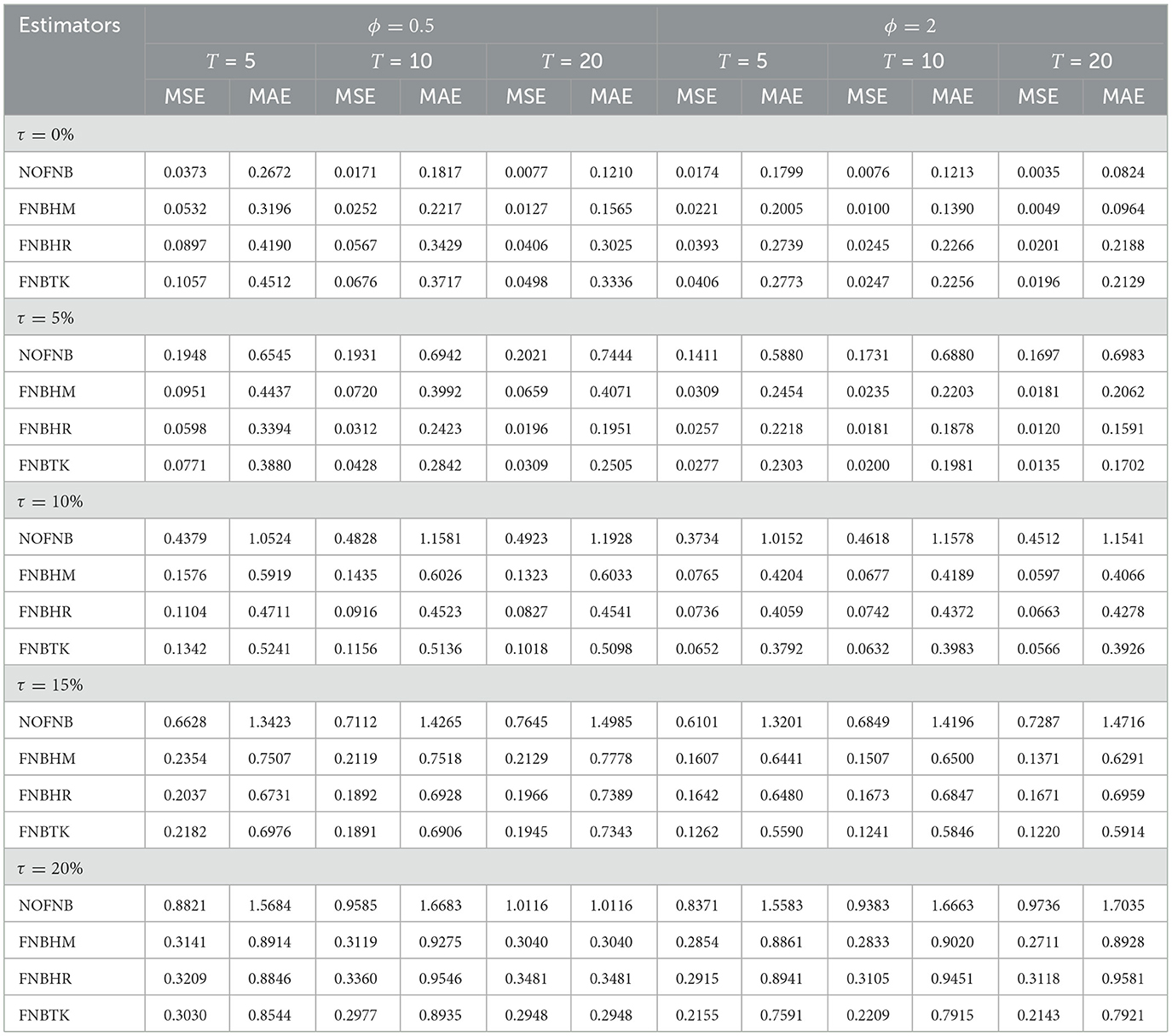
Table 3. MSE and MAE values of non-robust and robust estimates when N = 200.

Table 4

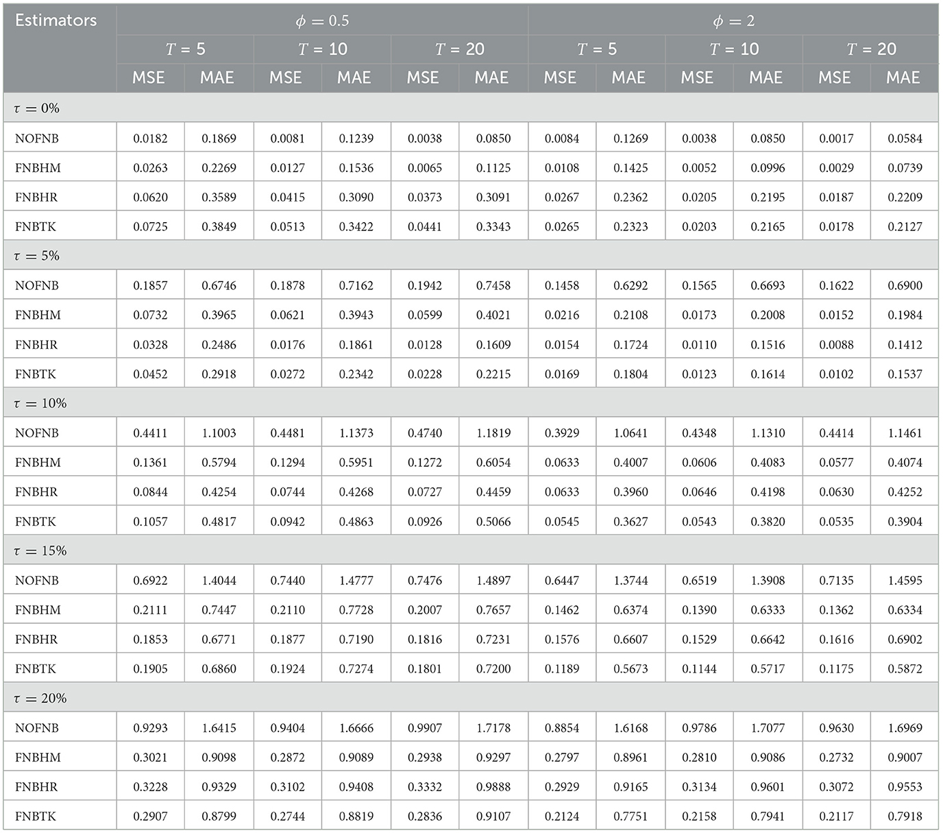
Table 4. MSE and MAE values of non-robust and robust estimates when N = 400.

In the context of clean data free from outliers (τ = 0%), the NOFNB estimator consistently performs better than the proposed estimators (FNBHM, FNBHR, and FNBTK) across all cases of N, T, and ϕ. This suggests that under ideal data conditions, the classical CML method offers higher efficiency. For example, at N = 50, ϕ = 0.5, T = 5, and τ = 0%, the MSE of the NOFNB estimator is 0.1614, whereas the values for FNBHM, FNBHR, and FNBTK are 0.2331, 0.2758, and 0.3345, respectively.

In contrast, when the data contain outliers (τ > 0%), the FNBHM, FNBHR, and FNBTK estimators outperform the classical NOFNB estimator. The presence of outliers negatively affects the performance of NOFNB, leading to inflated error values, while the robust methods maintain greater stability and accuracy. For instance, at N = 200, ϕ = 2, T = 20, and τ = 10%, the MSE values of FNBHM, FNBHR, and FNBTK are 0.0597, 0.0663, and 0.0566, respectively, compared to 0.4512 for NOFNB.

Moreover, as the proportion of outliers increases, both MSE and MAE tend to rise; however, the rate of increase is slower for the proposed estimators than for the NOFNB. For example, when τ increases from 10 to 15% at N = 100, ϕ = 2, and T = 10, the MAE values of FNBHM, FNBHR, and FNBTK increase from 0.4100, 0.4087, and 0.3826 to 0.6216, 0.6759, and 0.5661, respectively, while the MAE of NOFNB jumps from 1.0490 to 1.4436. These results highlight the greater robustness of the proposed estimators in the presence of outliers.

As the number of cross-sectional units increases from N = 50 to N = 400, the values of MSE and MAE generally decrease for all estimators, indicating enhanced estimation accuracy due to the larger unit's size and increased information. For example, when T = 10, τ = 5%, and ϕ = 2, the MSE of the classical estimator NOFNB decreases from 0.1871 at N = 50 to 0.1565 at N = 400. Similarly, for the proposed robust estimator FNBTK, the MSE drops from 0.0507 to 0.0123 over the same increase in N. This decreasing trend is consistently observed for both robust and non-robust estimators. However, robust estimators continue to offer more reliable estimates in the presence of outliers, regardless of the value of N. Although the classical estimator benefits significantly from increased sample size under clean data conditions, it becomes less reliable when the data contain outliers.

Increasing the time dimension (T) also enhances the performance of all estimators by providing more repeated observations over time. When holding N = 200, ϕ = 2, and τ = 10% fixed, increasing T from 5 to 20 leads to a noticeable reduction in both MSE and MAE values. For instance, the MSE of the proposed estimator FNBHM decreases from ~0.0765 at T = 5 to 0.0597 at T = 20, reflecting a substantial improvement in estimation precision. This trend highlights the importance of longer time-series dimensions in reducing estimation error, even in the presence of moderate levels of outliers. We also find that, when comparing the performance across both under-dispersion (ϕ = 0.5) and over-dispersion (ϕ = 2) scenarios, the robust estimators generally maintain their superiority in the presence of outliers.

The MRE for robust estimators (FNBHR, FNBHM, and FNBTK) is illustrated in Figures 1, 2 clustered by percentages of outliers (from 5 to 20%) and time-series (from 5 to 20) for all units separately. The evaluation was performed separately for two cases; the first case expresses under-dispersion (ϕ = 0.5), while the second case expresses over-dispersion (ϕ = 2).

Figure 1

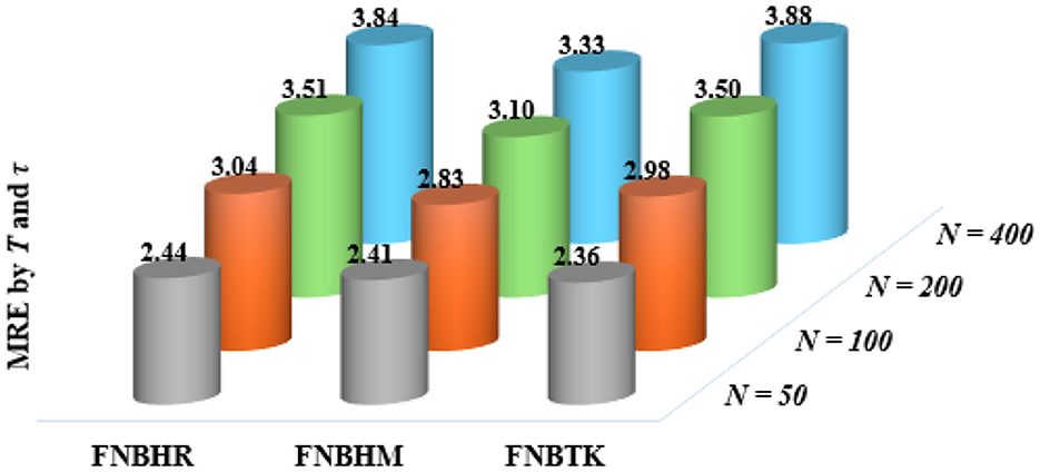
Figure 1. MRE of the robust estimates when ϕ = 0.5.

Figure 2

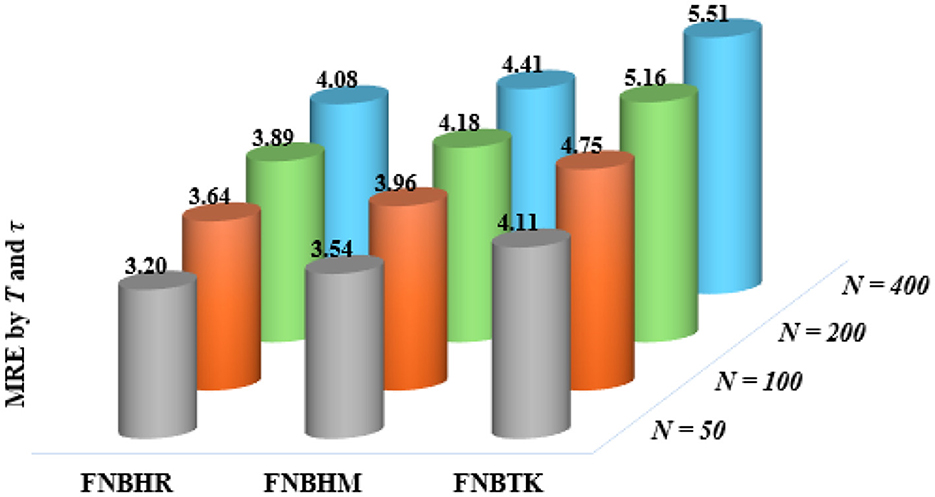
Figure 2. MRE of the robust estimates when ϕ = 2.

The results presented in Figures 1, 2 highlight the differences in estimators performance under varying dispersion levels. The efficiency of these estimators increases when increasing the size of the cross section (N), the time series (T), the percentage of the outliers (τ), and the dispersion parameter (ϕ), but the FNBTK estimator remains more efficient. Overall, the findings indicate that the MRE values of the FNBTK estimator are consistently higher than those of the FNBHR and FNBHM estimators. This suggests that the FNBTK estimator is more efficient than the other two robust estimators across all scenarios of N, T, τ, and ϕ.

4 Real-life panel data applications

The practical relevance of the proposed estimation methods is evaluated through real-life panel data applications from selected European countries, representing different types of count panel data frequently encountered in public health and economic contexts. To demonstrate the flexibility and robustness of these estimators under real-world conditions, two empirical case studies are presented. The first application utilizes COVID-19 data, while the second focuses on patent data, providing insights into the dynamics of innovation and economic development over time. Both datasets exhibit the panel structure necessary to evaluate the performance of classical and robust estimators under varying degrees of heterogeneity, over-dispersion, and the presence of outliers. Through these applications, the practical value and adaptability of the proposed methods are highlighted across real-world scenarios.

4.1 COVID-19 application

In recent years, the global emergence of COVID-19 has led to profound disturbances in healthcare systems, economic structures, and social dynamics worldwide. The availability of COVID-19-related data has played a pivotal role in facilitating research focused on understanding the virus's spread and evaluating the effectiveness of public health actions. Such data have proven essential for researchers, policymakers, and healthcare institutions striving to mitigate the pandemic's impact and address its multifaceted challenges.

Comprehensive and reliable COVID-19 datasets have provided a solid foundation for conducting empirical research. These datasets have not only enhanced our understanding of pandemic dynamics but have also spurred advancements in statistical modeling, particularly in the fields of count panel data analysis, panel data techniques, and robust estimation approaches. As a result, COVID-19 data have become instrumental in applying and validating modern statistical methods, promoting innovation in methodology, encouraging interdisciplinary collaboration, and contributing to the design of evidence-based policies. In this context, the use of such data highlights the practical relevance and empirical strength of the proposed estimation techniques, especially in addressing real-world problems associated with public health crises.

This application employs a daily panel dataset on COVID-19, covering ten European countries during the period from June 23, 2021, to January 21, 2022. The data were obtained from the World Health Organization website. The analysis includes five variables, with the response variable being the number of new COVID-19-related deaths (y_it). The explanatory variables are the number of confirmed cases per 1,000 individuals (X₁), the number of patients in intensive care units per 100 individuals (X₂), the logarithm of new COVID-19 tests (X₃), and the logarithm of the number of individuals who received COVID-19 vaccinations (X₄).

Figure 3 presents boxplots of the study variables that exhibit outliers across the selected countries. A visual examination of the boxplots reveals the presence of outliers in the y_it as well as in the explanatory variables: X₁, X₂, and X₃. Furthermore, an over-dispersion test was conducted, and the results indicated a statistically significant presence of over-dispersion in the data, with a p-value < 0.001.

Figure 3

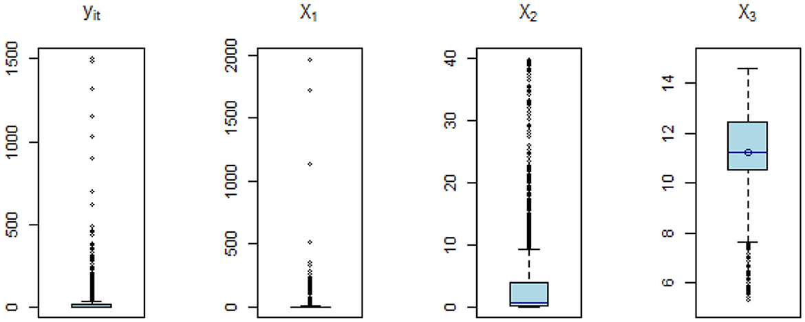
Figure 3. Box plots of COVID-19 variables containing outliers.

The algorithm described in Section 2 is applied to obtain the estimators' results, aiming to derive more accurate estimates and enhance the robustness and reliability of the analysis. Table 5 presents the coefficient estimates from the NB panel model using both non-robust and robust methods. The results in Table 5 summarize the estimated coefficients for the NB panel model applied to the COVID-19 dataset. The NOFNB estimator, which does not account for outliers, produces significantly different coefficient values compared to the robust estimators.

Table 5

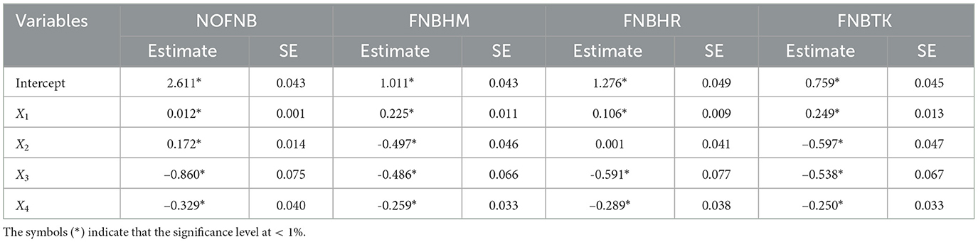
Table 5. Coefficient estimates for various estimators using the COVID-19 dataset.

To evaluate the performance of these estimators, we refer to the goodness-of-fit measures reported in Table 6. These measures clearly show that the robust estimators yield lower values for AIC and BIC, demonstrating their superior performance. Among them, the FNBTK estimator achieves the lowest values across all criteria, confirming its effectiveness in handling outliers in count panel data.

Table 6

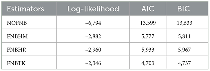
Table 6. Goodness-of-fit measures for the estimators in COVID-19 dataset.

4.2 Patents application

Another empirical application is conducted to evaluate the performance of the proposed estimators using patents data. In the global economy, patents stand as cornerstones of innovation, economic growth, and competitive advantage, particularly in high-income European countries. These countries have long recognized the real value of intellectual property rights in creating an environment that supports and promotes research, development, and marketing the new ideas. Patents, by providing exclusive rights to inventors for a defined period, encourage the development and dissemination of innovative technologies, thus propelling advancements in various sectors including healthcare, information technology, and green energy. Moreover, in the context of the European single market, patents play a pivotal role in harmonizing standards, facilitating cross-border trade, and enhancing the region's attractiveness to investors and entrepreneurs from around the globe. Consequently, understanding the importance of patent protection in these countries is a crucial element in comprehending their economic resilience and their ability to find pioneering solutions to global challenges. In this context, we will employ the patents dataset to evaluate various estimators.

In our application, we are interested in estimating patent applications. As defined by the World Intellectual Property Organization, a patent application is associated with either a new method of operation or a novel technical problem solution. We based our sample selection on the patent data for high-income European countries available on the World Bank website. This sample includes 17 countries classified as high-income, covering the years from 2005 until 2020. In this analysis, we focus on the patents (PATEN) as the dependent variable. The independent variables are the number of researchers in research and development (NUMRD) per 1000 people, the logarithm of the research and development expenditures (RDEXD), the logarithm of the GDP per capita (GDPPC), the logarithm of the exports of technological goods (ICTEXP), and the rate of unemployment (UNEMP).

Figure 4 displays box plots for the variables that exhibit outliers across the countries under study. Specifically, the box plots indicate that the response variable and UNEMP contain outlier values, while the remaining variables do not show apparent outliers. Also, we conducted an over-dispersion test and the results indicated a significant presence of over-dispersion in the data < 0.001 significance level. Table 7 shows the findings of the NB panel model of non-robust and robust estimates.

Figure 4

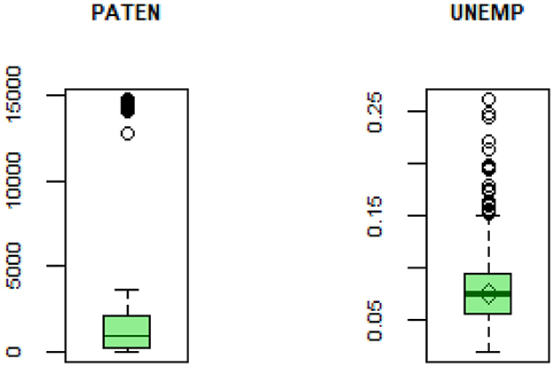
Figure 4. Box plots of patent variables containing outliers.

Table 7

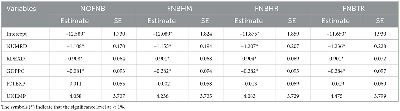
Table 7. Coefficient estimates for various estimators using the patent dataset.

After assessing the AIC and BIC criteria, as illustrated in Table 8, to a conclusion that robust estimates for the NB panel model outperformed non-robust estimates in terms of effectiveness, which indicates that the robust estimators FNBHM, FNBHR, and FNBTK outperform when compared to the NOFNB non-robust estimator. The criterion for determining the best estimator relies on selecting the one with the lowest value for either AIC or BIC. This finding emphasizes the importance of selecting robust estimators for enhanced accuracy and reliability in evaluating the results. In addition, the FNBTK estimator demonstrates better performance compared to the other estimators. The findings clearly demonstrate that robust estimators outperform classical estimator when outliers are present.

Table 8

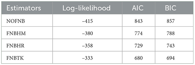
Table 8. Goodness-of-fit measures for the estimators in patent dataset.

5 Conclusion

In this research study, we have presented proposed robust estimators for the FENB panel model. To evaluate the performance of these estimators, we conducted the simulation study and applied them to real panel datasets. By combining Monte Carlo simulation and the applications of real data, we can conduct a comprehensive evaluation of the proposed estimators, ensuring their effectiveness and reliability. This dual approach allows us to assess the estimators' performance across different situations, providing a comprehensive understanding of their robustness and practical utility under diverse conditions.

The simulation results indicate that in the absence of outliers, the NOFNB estimator outperforms the robust estimators, but, when outliers are present, the proposed robust estimators (FNBHM, FNBHR, and FNBTK) exhibit higher effectiveness compared to the non-robust estimator. Furthermore, the results of the empirical studies in European countries indicate that the proposed robust estimators are more efficient than other estimators when outliers are present in the datasets. In addition, the FNBTK robust estimator demonstrates greater efficiency compared to FNBHM and FNBHR robust estimators.

The results of this study are expected to have practical implications for researchers and policymakers in the field of scientific research and development. In addition, it contributes to the advancement of statistical methodology for analyzing count panel data in the presence of outliers and provides a better understanding of the factors influencing count panel data in different fields by emphasizing the importance of the NB panel model. In future work, we plan to propose new robust estimators for the FENB model or for one of the other count panel data models.

Data availability statement

Publicly available datasets were analyzed in this study. The first data can be found at: https://www.who.int/data. The second data can be found at: https://databank.worldbank.org/. The files for both datasets are found in the Supplementary material.

Author contributions

MA: Formal analysis, Investigation, Methodology, Resources, Software, Validation, Visualization, Writing – original draft, Writing – review & editing. EE: Funding acquisition, Investigation, Methodology, Project administration, Resources, Software, Supervision, Validation, Writing – review & editing. EA: Conceptualization, Data curation, Formal analysis, Investigation, Methodology, Resources, Validation, Visualization, Writing – original draft, Writing – review & editing. AE-M: Data curation, Funding acquisition, Investigation, Project administration, Resources, Software, Supervision, Visualization, Writing – review & editing.

Funding

The author(s) declare that no financial support was received for the research and/or publication of this article.

Conflict of interest

The authors declare that the research was conducted in the absence of any commercial or financial relationships that could be construed as a potential conflict of interest.

Generative AI statement

The author(s) declare that no Gen AI was used in the creation of this manuscript.

Any alternative text (alt text) provided alongside figures in this article has been generated by Frontiers with the support of artificial intelligence and reasonable efforts have been made to ensure accuracy, including review by the authors wherever possible. If you identify any issues, please contact us.

Publisher's note

All claims expressed in this article are solely those of the authors and do not necessarily represent those of their affiliated organizations, or those of the publisher, the editors and the reviewers. Any product that may be evaluated in this article, or claim that may be made by its manufacturer, is not guaranteed or endorsed by the publisher.

Supplementary material

The Supplementary Material for this article can be found online at: https://www.frontiersin.org/articles/10.3389/fams.2025.1638596/full#supplementary-material

References

1. Ahmed EG, Abonazel MR, Al-Ghamdi MN, Elshamy HM, Khattab IG. Proposed robust estimators for the Poisson panel regression model: application to COVID-19 deaths in Europe. Commun Math Biol Neurosci. (2024) 2024:121. doi: 10.28919/cmbn/8795

Crossref Full Text | Google Scholar

2. Abonazel MR, Youssef AH, Ahmed EG. On robust M, S and MM estimations for the Poisson fixed effects panel model with outliers: simulation and applications. J Stat Comput Simul. (2025) 95:1190–207. doi: 10.1080/00949655.2024.2449102

Crossref Full Text | Google Scholar

3. Youssef AH, Abonazel MR, Ahmed EG. Robust M estimation for Poisson panel data model with fixed effects: method, algorithm, simulation, and application. Stat Optim Inf Comput. (2024) 12:1292–305. doi: 10.19139/soic-2310-5070-1996

Crossref Full Text | Google Scholar

4. Baltagi BH. Econometric Analysis of Panel Data. Hoboken, NJ: John Wiley and Sons Ltd (2005).

Google Scholar

5. Abonazel MR, Ahmed EG, El-Baz ST, Ebrahim EEM. How economic policies drive climate change: a comparative analysis of groups of middle- and high-income countries. Int J Energy Econ Policy. (2025) 15:447–55. doi: 10.32479/ijeep.17853

Crossref Full Text | Google Scholar

6. Winkelmann R. Econometric Analysis of Count Data. Berlin: Springer-Verlag. (2008).

Google Scholar

7. Cameron AC, Trivedi PK. Regression Analysis of Count Data. Cambridge: Cambridge University Press (2013). doi: 10.1017/CBO9781139013567

Crossref Full Text | Google Scholar

8. Yaacob WFW, Lazim MA, Wah YB. A practical approach in modelling count data. In: Proceedings of the Regional Conference on Statistical Sciences. Shah Alam: Malaysia Institute of Statistics, Faculty of Computer and Mathematical Sciences, University Technology MARA (UiTM) (2010). p. 176–183.

Google Scholar

9. Hana N. Negative binomial regression model for road crash severity prediction. Mod Appl Sci. (2018) 12:38–46. doi: 10.5539/mas.v12n4p38

Crossref Full Text | Google Scholar

10. Al-Taweel Y, Algamal Z. Some almost unbiased ridge regression estimators for the zero-inflated negative binomial regression model. Period Eng Nat Sci. (2020) 8:248–55. doi: 10.21533/pen.v8i1.1107

Crossref Full Text | Google Scholar

11. Alobaidi NN, Shamany RE, Algamal ZY. A new ridge estimator for the negative binomial regression model. Thailand Stat. (2021) 19:115–24.

Google Scholar

12. Rashad NK, Hammood NM, Algamal ZY. Generalized ridge estimator in negative binomial regression model. J Phys Conf Ser. (2021) 1897:012019. doi: 10.1088/1742-6596/1897/1/012019

Crossref Full Text | Google Scholar

13. Niang MA, Diop A, Seck CT, Faye I, Ndao A, Sy IA, et al. negative binomial regression analysis for COVID-19 death cases in Senegal. Int J Stat Appl Math. (2022) 7:6–12. doi: 10.22271/maths.2022.v7.i3a.817

Crossref Full Text | Google Scholar

14. Liu R, Heo I, Liu H, Shi D, Jiang Z. Applying negative binomial distribution in diagnostic classification models for analyzing count data. Appl Psychol Meas. (2023) 47:64–75. doi: 10.1177/01466216221124604

PubMed Abstract | Crossref Full Text | Google Scholar

15. Suryadi F, Jonathan S, Jonatan K, Ohyver M. Handling overdispersion in Poisson regression using negative binomial regression for poverty case in West Java. Procedia Comput Sci. (2023) 216:517–23. doi: 10.1016/j.procs.2022.12.164

Crossref Full Text | Google Scholar

16. Youssef AH, Abonazel MR, Ahmed EG. Estimating the number of patents in the world using count panel data models. Asian J Probab Stat. (2020) 6:24–33. doi: 10.9734/ajpas/2020/v6i430167

Crossref Full Text | Google Scholar

17. Kumara SSP, Chin HC. Study of fatal traffic accidents in Asia Pacific countries. Transp Res Rec. (2004) 1897:43–7. doi: 10.3141/1897-06

PubMed Abstract | Crossref Full Text | Google Scholar

18. Guimaraes P. The fixed effects negative binomial model revisited. Econ Lett. (2008) 99:63–6. doi: 10.1016/j.econlet.2007.05.030

PubMed Abstract | Crossref Full Text | Google Scholar

19. Hausman JA, Hall BH, Griliches Z. Econometric models for count data with an application to the patents-R&D relationship. Econometrica. (1984) 52:909–38. doi: 10.2307/1911191

PubMed Abstract | Crossref Full Text | Google Scholar

20. Youssef AH, Abonazel MR, Ahmed EG. The performance of count panel data estimators: a simulation study and application to patents in Arab countries. J Math Comput Sci. (2021) 11:8173–96. doi: 10.28919/jmcs/5852

PubMed Abstract | Crossref Full Text | Google Scholar

21. Huber P. Robust estimation of a location parameter. Ann Math Stat. (1964) 35:73–101. doi: 10.1214/aoms/1177703732

Crossref Full Text | Google Scholar

22. Huber PJ. Robust Statistics. Hobokn, NJ: John Wiley & Sons (1981). doi: 10.1002/0471725250

Crossref Full Text | Google Scholar

23. Rousseeuw PJ, Leroy AM. Robust Regression and Outlier Detection. Hobokn, NJ: John Wiley & Sons (1987). doi: 10.1002/0471725382

Crossref Full Text | Google Scholar

24. Garay AM, Hashimoto EM, Ortega EMM, Lachos VH. On estimation and influence diagnostics for zero-inflated negative binomial regression models. Comput Stat Data Anal. (2011) 55:1304–18. doi: 10.1016/j.csda.2010.09.019

PubMed Abstract | Crossref Full Text | Google Scholar

25. Toka O, Cetin M. The comparing of S-estimator and M-estimators in linear regression. Gazi Univ J Sci. (2011) 24:747–52.

Google Scholar

26. Susanti Y, Pratiwi H, Sulistijowati S, Liana T. M estimation, S estimation, and MM estimation in robust regression. Int J Pure Appl Math. (2014) 91:349–60. doi: 10.12732/ijpam.v91i3.7

Crossref Full Text | Google Scholar

27. Maronna RA, Martin RD, Yohai VJ. Robust Statistics: Theory and Methods. Hoboken, NJ: John Wiley & Sons (2019). doi: 10.1002/9781119214656

Crossref Full Text | Google Scholar

28. Tüzen F, ErbaŞ, OlmuŞ H. A simulation study for count data models under varying degrees of outliers and zeros. Commun Stat-Simul Comput. (2020) 49:1078–1088. doi: 10.1080/03610918.2018.1498886

Crossref Full Text | Google Scholar

29. Youssef AH, Abonazel MR, Kamel AR. Efficiency comparisons of robust and non-robust estimators for seemingly unrelated regressions model. WSEAS Trans Math. (2022) 21:218–44. doi: 10.37394/23206.2022.21.28

Crossref Full Text | Google Scholar

30. Ke S, Phillips PC, Su L. Robust inference of panel data models with interactive fixed effects under long memory: a frequency domain approach. J Econom. (2024) 241:105761. doi: 10.1016/j.jeconom.2024.105761

Crossref Full Text | Google Scholar

31. Beyaztas BH, Bandyopadhyay S. Data driven robust estimation methods for fixed effects panel data models. J Stat Comput Simul. (2022) 92:1401–25. doi: 10.1080/00949655.2021.1996576

PubMed Abstract | Crossref Full Text | Google Scholar

32. Amelia M, Sadik K, Sartono B. The study of robust estimators on panel data regression model for data contaminated with outliers. In: Proceedings of the 1st International Conference on Statistics and Analytics, Bogor, Indonesia, 2-3 August 2019. Bogor (2020). doi: 10.4108/eai.2-8-2019.2290517

Crossref Full Text | Google Scholar

33. Víšek JÁ. Estimating the model with fixed and random effects by a robust method. Methodol Comput Appl Probab. (2015) 17:999–1014. doi: 10.1007/s11009-014-9432-5

Crossref Full Text | Google Scholar

34. Bramati MC, Croux C. Robust estimators for the fixed effects panel data model. Econometr J. (2007) 10:521–40. doi: 10.1111/j.1368-423X.2007.00220.x

Crossref Full Text | Google Scholar

35. Hampel F, Ronchetti E, Rousseeuw P, Stahel W. Robust Statistics: The Approach Based on Influence Functions. Hoboken, NJ: John Wiley & Sons (1986).

Google Scholar

36. Venables WN, Ripley BD. Modern Applied Statistics with S, 4th Edn. Cham: Springer (2002). doi: 10.1007/978-0-387-21706-2

Crossref Full Text | Google Scholar

37. Baltagi BH. The Oxford Handbook of Panel Data. Oxford Handbooks. Oxford: Oxford University Press (2015). doi: 10.1093/oxfordhb/9780199940042.001.0001

Crossref Full Text | Google Scholar