Directed graph theory for the analysis of biological regulatory networks

Synchronous regulated biological networks are often represented as logical diagrams, where the precise interactions between elements remain obscured. Here, we introduce a novel type of excitation-inhibition graph based on Boolean logic, which we term “logical directed graph” or simply, “logical digraph.” Such a logical digraph facilitates the representation of every conceivable regulatory interaction among elements, grounded in Boolean interactions. The logical digraph includes information about connectivity, dynamics, limit cycles, and attractors of the network. As proof of application, we utilized the logical digraph to analyze the operations of the well-known neural network that produces oscillatory swimming in the mollusk Tritonia. Our method enables a seamless transition between a regulatory network and its corresponding logical digraph, and vice versa. Additionally, we demonstrate that the spectral properties of the so-called state matrix provide mathematical evidence explaining why the elements within attractors and limit cycles contain information about the dynamics of the biological system. More specifically, the non-zero entries of the Perron-Frobenius eigenvector of the state matrix indicate the attractors and limit cycles of the network. We demonstrate that each connected component of the regulatory network has exactly one attractor or limit cycle. Open software routines are available for calculating the components of the network, as well as the attractors and limit cycles. This approach opens new possibilities for visualizing and analyzing regulatory networks in biology.

1 Introduction

Synchronous regulatory networks in biology are formed when a collection of elements, such as molecules, neurons, or individuals, interact with one another to determine a dynamic system in discrete time steps. The overall behavior of a synchronous network is governed by a specific transition function. Detailed experimental investigations into the workings of synchronous regulatory networks can be enhanced by mathematical models that replicate the network's behavior, aiding in the development of new hypotheses and experiments. In this article, we present a quantitative method based on Boolean algebra to replicate behaviors and identify missing elements within the network.

Regulatory networks are typically studied by illustrating interactions among elements in the network using an excitation-inhibition graph [1–9]. For example, a and b represent two interacting elements, each having a binary Boolean behavior. We may now suppose that activation of a turns b on. Such activation, or excitation, can be described as a → b. If by contrast, a inhibits b, the expression will be a ⊣ b. That simple description can now be enriched in Boolean terms by using 1 to indicate an active state and 0 to indicate an inactive or inhibited state. However, this notation alone is insufficient to explain more sophisticated interactions. For example, element a may be activated when element b is inhibited. Alternatively, element a may remain unchanged upon activation of element b. Such naturally occurring interactions cannot be described solely by the excitatory and inhibitory connections. An alternative approach to describing networks and circuits in biology is to use the logical electrical diagrams commonly employed in engineering. However, these diagrams act as black boxes, where the precise interactions between the elements remain concealed from sight [5].

To overcome these limitations, we propose a digraph (directed graph) that we will refer to as a logical digraph of the biological system. The logical digraph is constructed using eight logical connectives and their combinations, representing every possible interaction between any two elements. When combined with appropriate Boolean functions, the digraph accurately defines the dynamics of the biological regulatory system. In addition to being algorithmic, our method reports on the system's attractors and limit cycles, which correspond to the Perron-Frobenius eigenvectors of the state matrix that describes the transition from one state to another over time. Therefore, the state matrix contains information about the dynamics of the biological network [10]. As new concepts arise throughout the paper, they are applied to the simple neural circuit that controls swimming in the mollusk Tritonia to exemplify the use of the logical digraph.

2 The logical digraph of a regulatory biological system. Definitions and basic notions

A regulatory biological system and its dynamics can be described by the quartet of symbols ($\mathcal{G}$, $\mathcal{S}$, F, η). The symbol $\mathcal{G}$ ={g₁,…,g_n} represents a finite assembly of n elements (genes, neurons, cells, or nodes), each of which can acquire either the Boolean active state (on, true) with a value of 1, or the inactive state (off, false) with a value of 0. We will denote the set of Boolean values as Z₂ = {0,1}, along with their usual Boolean operations: addition (⊕) and multiplication (⊗), which are described in Table 1. The glossary contains definitions of the terms.

Table 1

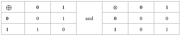
Table 1. Values of the Boolean sum and multiplication of two interacting elements in a regulatory network.

In the set ${\mathbb{Z}}_2^n$ = {(a₁, …, a_n): a_i ∈ ℤ₂ for each j=1,…,n} the j-th coordinate corresponds to the element g_j of $\mathcal{G}$. This set contains all the possible states (0,1) of the elements of $\mathcal{G}$, which we will refer to as state-vectors. All the state-vectors of biological system are contained in $\mathcal{S},$ which is a subset of ${\mathbb{Z}}_2^n.$

The symbol η represents the regulatory network as a digraph whose vertices are the state vectors (the elements of $\mathcal{S}$). η informs about the time-evolution of the regulatory cycle. In the expression (a₁, …, a_n) → (b₁, …, b_n), the arrow means that the state (a₁, …, a_n) changes to the state (b₁, …, b_n) in a time unit. These changes are described by the transfer function F= (f₁,…, f_n) of the system, and can be defined by n Boolean functions f_j: ${\mathbb{Z}}_2^n\to {\mathbb{Z}}_2$that describe how the elements of $\mathcal{G}$ act on element g_j. In other words, the transfer function F goes from ${\mathbb{Z}}_2^n$to ${\mathbb{Z}}_2^n$ and the arrow (a₁, …, a_n) → (b₁, …, b_n) in η means the transfer function (b₁, …, b_n)= F(a₁, …, a_n).

3 Logical connectives

We can now proceed by employing logical connectives that indicate excitation and inhibition. To begin, we will again use the excitation connective to clarify the essentials of utilizing connectives:

1. Excitation. An active a (a = 1) induces the transition of b from inactive (b = 0) to active (b = 1). The binary value 1 represents excitation from a to b, and is represented as a → b. However, the excitation value depends on the initial states of either component. As shown in Table 2, connective a → b, if a is off (a = 0), b will remain inactive (b = 0). Note, however, that if b is initially active, the activation of a also provides a 1 value. In contrast, the initial value of b remains unchanged when a = 0.

Table 2

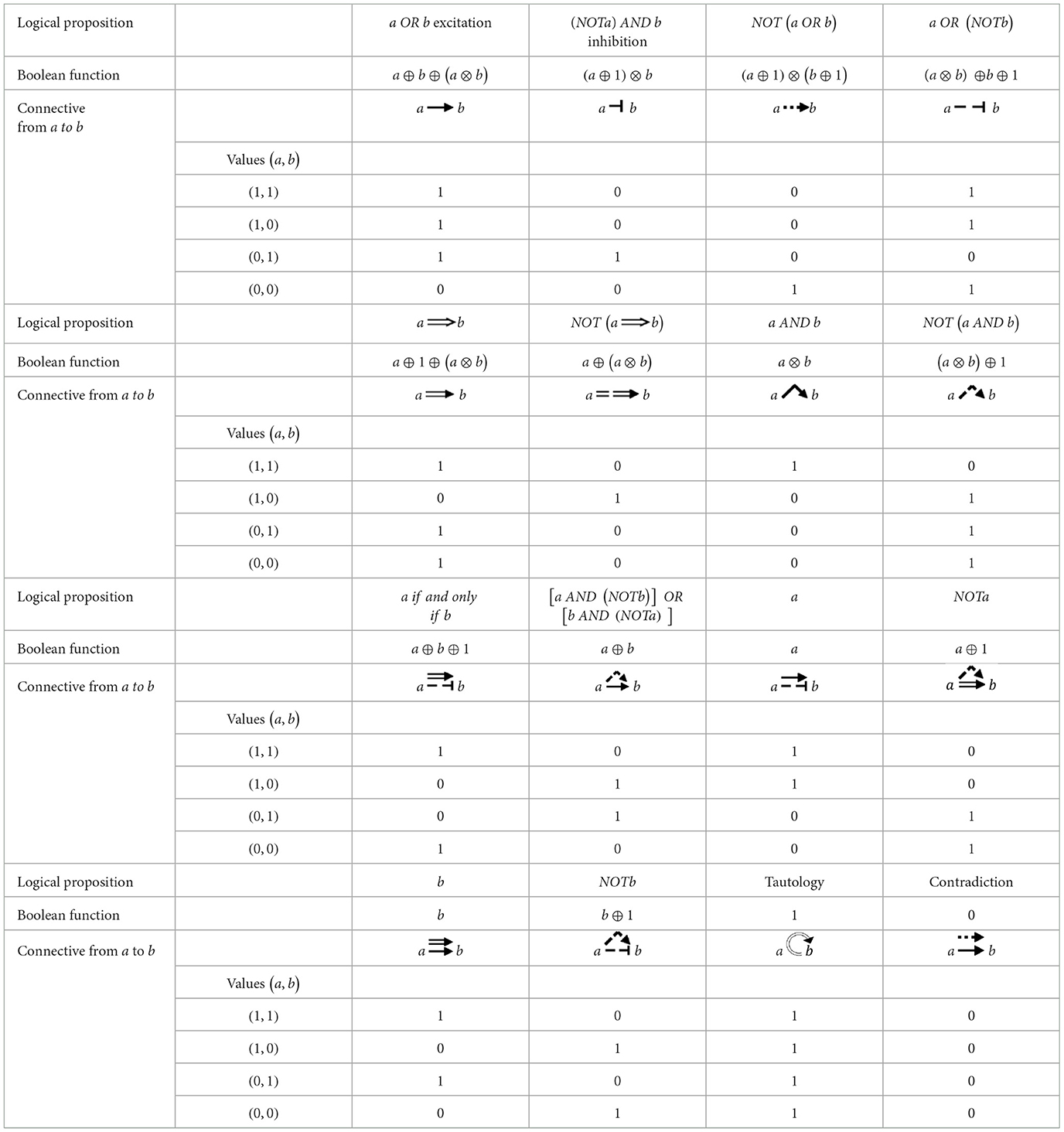
Table 2. Connectives, logical propositions, Boolean functions and the values of the 16 actions from a to b.

3.1 The identity of a

It is used when a does not change in time. Its logical connective is a → a or the lace in a, .

As an equivalent to describe the identity in a, we may use one of the following logical connectives, or or or . This connective express that the interaction of gene Sp8 to its product protein Sp8 remains constant over time during development of the mammalian cerebral cortex ([11], P. 3).

2. Inhibition, a ⊣ b. In direct inhibition, the activity of a turns b off. Therefore, the a = 1 value when a is active, produces b = 0. Alternatively, if a is inactive b remains unaffected. That is, b preserves its original value.

4 More logical connectives

The complexity of biological interactions extends well beyond mere excitation or inhibition. The various ways in which a may affect b depend on the current state of each interactive element. Furthermore, one must consider global activity even when a is inactive, a fact not always considered in this type of analysis. For this reason, six additional connectives must be included to represent the dynamics of real biological regulation networks accurately. Although some have not been biologically described, we consider all the possible interactions between connectives. Since regulatory networks commonly have undefined components, such connectives may serve to hypothesize identities and interactions.

3. Negation of excitation . A first case occurs if activation of a inhibits an initially active b, that is (1 1) = 0. In a second case, b remains inactive during the activity of a, (1 0) = 0. Both cases resemble the inhibition seen above. However, here the inactivity of a produces inactivation of b, (0 b) = 0. Alternatively, the initial inactivity of both a and b produces activation of b, (0 0)= 1. Note that this connective differs from inhibition. As an example, the identity of gen Sp8 in Giacomantonio and Goodhill [11], p. 3, can be described as [Emx2 Fgf8] Sp8 .

4. Negation of inhibition . Unlike the previous case, any difference in the initial activity between a and b leads to a change in the b value. However, inactivity in both a and b, keeps b inactive.

5. Implication . The activity in both a and b, keeps b active. In contrast, the inactivity of a produces spontaneous activation of b; in the other cases, b will remain inactive.

6. Negation of implication . Unlike the implication, the only case where b is activated is when a is active and b is inactive. As an example, in Giacomantonio and Goodhill [11] F(t) ==> E(t), which is equivalent to F(t) & NOT E(t).

7. Disjunction . The activity of b requires the simultaneous activity of a and b. This connective, also read as a AND b, is the most abundant in literature. For example, [(NOT Emx2) Fgf8] Sp8 indicates that the value of Sp8 is the disjunction of (NOT Emx2) and Fgf8 ([11], p. 3).

8. Negation of disjunction . b becomes inactive when both a and b are simultaneously active.

5 Combining logical connectives

So far, the interactions between the two elements have been characterized by a single symbol. The following eight complex interactions will be defined by a combination of two or more logical connectives connected by the logical connective “AND” (or disjunction).

9. Double implication or If and only if. It is represented as a b AND a b or simply as a b. Means that b will be active if a and b have the same value (see 3.1).

10. Negation of the double implication . Its representation is a b AND a b. This means that alternating the values of a and b will activate b.

11. “a” as an action from a to b (ab). Means that regardless of its value, b takes the value of a. See also Section 3.1.

12. “NOT a” (as an action from a to b) or Negation of a . Regardless of the value of a, b takes the opposite, as shown in the logical diagram of the regulatory system of Tritonia (Figure 3).

13. “b” (as an action from a to b) (a b). That is, the value of b remains invariant. This connective may be useful to test whether an element does not influence a biological system or if any other connective is needed. The appearance of this connective suggests that removing a might be possible because it is redundant. In other case, when we know that a interacts with b, the appearance of this connective indicates the presence of another element acting from a to b. See also Section 1.1.

14. “NOT b” (as an action from a to b) (a b). Means that b takes on a value that is opposite to its original value, independently of the value of a. For example, b b means autoinhibition of b.

15. Tautology (as an action from a to b) (a ), b will always be activated. As will be seen in the example below, this connective is used for autoexcitation of b as an alternative to the filled circles used in Cessac and Samuelides ([12], Figure 63).

16. Contradiction (as an action from a to b) (a b). Means that b will always be inactivated. One use of this connective is the autoinhibition of b [see also Cessac and Samuelides [12], Figure 63].

Table 2 summarizes the connectives, their logical propositions, Boolean functions, and values. The strategy now is to define the logical proposition for each Boolean function in n variables, along with the corresponding logical digraph and vice versa.

6 Bijection between logical propositions and Boolean functions

To represent the regulatory network in Boolean terms, we need to convert logical propositions into Boolean functions. This connection can be established if a bidirectional equivalence, also known as tautology, exists, which means that the conversion holds true under every possible interpretation. For example, the two logical propositions P and Q are equivalent if the logical proposition “P if and only if Q” is a tautology. Table 2 shows that the truth table of the connective excitation, a b, is identical to the logical proposition OR, indicating that their Boolean propositions are also the same. Therefore, a tautology exists, allowing us to substitute one for the other.

Table 3 shows a bijection between the set of logical propositions in n variables and the set of Boolean functions from ${\mathbb{Z}}_2^{n}to{\mathbb{Z}}_2$, for each natural number n ≥ 1.

Table 3

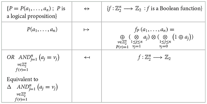
Table 3. Bijections between a set of logical propositions with n variables and the corresponding set of Boolean functions.

7 From a regulatory biological system to its logical digraph and vice versa

We will now return to the synchronous biological regulatory system $(\mathcal{G},\mathcal{S},F,\eta )$ and will use η to build the transfer function F (alternatively, we can use F to build η). The Supplementary material contains a computer routine that calculates the function F from a predefined regulatory network η.

The logical digraph of a biological regulatory system ($\mathcal{G},\mathcal{S},F,\eta$) has one vertex for each of the n elements of $\mathcal{G}$. Such vertices will be denoted as g₁, …, g_n ($\mathcal{G}=\left\{g_1,\dots ,g_n\right\})$, and the directed connectives joining the vertex correspond to the logical connectives in Table 2. $\mathcal{S}$ is the set of state-vectors and F = (f₁, …, f_n) is the set of Boolean functions that define the regulatory network η. The glossary at the end defines each term in the text.

7.1 Attractors and limit cycles

Roughly speaking, an attractor is a directed loop, while a limit cycle is a directed cycle of length at least 2 in the regulatory network. That is, attractors and limit cycles are minimal sets of states from which no escape is possible.

It is now necessary to describe each Boolean function $f_i:{\mathbb{Z}}_2^n\to {\mathbb{Z}}_2$ in terms of the sum and multiplication of ℤ₂, such that:

$\begin{array}{c}{f}_i(a_1,\dots ,a_n)={\displaystyle \underset{\begin{array}{c}v\in {\mathbb{Z}}_2^n\\ f_i(v)=1\end{array}}{\oplus }}\left(\underset{\begin{array}{c}1\le j\le n\\ v_j=1\end{array}}{\otimes }{a}_j\underset{\begin{array}{c}1\le j\le n\\ v_j=0\end{array}}{\otimes }(1\oplus a_j)\right)\end{array}$

To obtain its corresponding logical proposition P_i we apply the bijection to each Boolean function f_i of F, (see Table 3). From Table 2, we will obtain the logical connectives for every element in $\mathcal{G}$ (including g_i) to the vertex g_i. Keep in mind that the logic digraph is constructed from all the interactions among the elements, including those formed by an element acting on itself.

8 Application of the logical digraph to analyze the neural network of swimming in a mollusk

The well-known and relatively simple neural network controlling swimming of the mollusk Tritonia offers numerous advantages for testing mathematical network theory applied to animal behavior [13]. Like in other invertebrates, swimming in Tritonia is produced by a sequence of sigmoidal body waves occurring during alternate cycles of contraction of the ventral and dorsal muscles. The beauty of such neuronal circuitry lies in the combination of its simplicity and the reproducibility of the emerging behavior. Studies conducted by Getting, Katz, and others [1, 13–17] have shown that swimming is produced by a central pattern generator integrated by four types of central neurons that establish a stereotyped connectivity.

Motoneurons transmit output information that alternates the contraction of dorsal and ventral muscles. In brief, activation of the Dorsal Interneuron (DI) generates bursts of action potentials that activate the dorsal motoneurons through excitatory connections. Swimming begins in the upward direction. Simultaneously the DI neuron activates the cerebral type 2 (C2) neuron. The C2 neuron responds with a stream of impulses that produce a delayed excitation of the ventral interneurons (VI). Two types of VI neurons cooperate to the pattern; however, for this study, it suffices to condense both into a single representative neuron (see also Tamvacakis et al. [18]). The VI interneuron connects to the ventral motoneurons, which cause the ventral contraction of the animal [19].

As of now, only direct excitatory and inhibitory connections have been identified. However, the timing of the cyclic activation of the CPG necessitates additional connections. Reciprocal inhibitory connections between the DI and VI motoneurons are crucial. The DI and VI interneurons communicate with one another through reciprocal inhibitory connections (Figure 1). The activity of DI neurons suppresses VI neurons, clearing the circuit to produce a single dorsal output while prolonging the excitation period of the dorsal motoneurons. Moreover, the excitation of C2 neurons, followed by the excitation of VI neurons, inhibits DI and C2 interneurons, allowing a singular ventral output from the circuit. A third type of connection that contributes to the duration of the burst of impulses by the DI and VI motoneurons is excitatory autapses—specifically, synaptic connections that neurons form onto themselves. Activation of autapses during bursts of action potentials extends the excitation of the DI or VI neurons, thereby lengthening the duration of their firing and creating inhibition of the antagonistic neuron. The network in Figure 1A is a basic description that utilizes only the excitation and inhibition connectives to describe the interactions between the three neuron types.

Figure 1

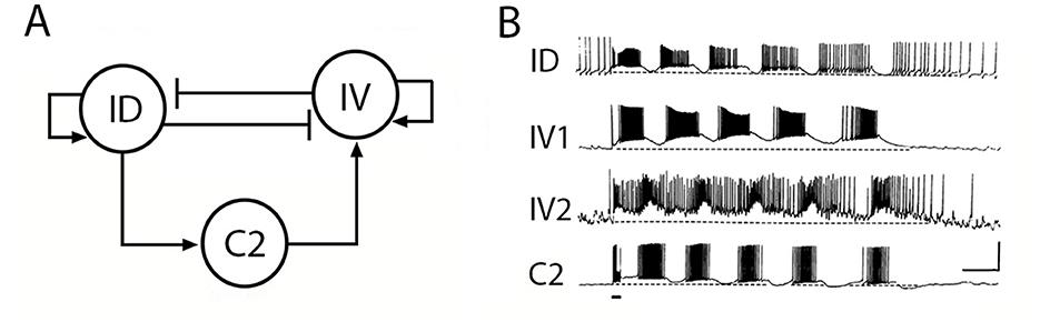
Figure 1. The neuronal circuit of swimming in Tritonia. (A) The basic neuronal circuit that integrates the CPG. DI, dorsal interneuron; VI, ventral interneurons; C2, cerebral neuron type 2. The DI and VI interneurons connect directly to their respective motoneurons (not shown). Excitatory connections are indicated by the vertical small bars, while inhibitory connections are represented by circles. The small bar below denotes the swimming-initiating stimulus. (B) Simultaneous intracellular recordings from each type of neuron. Note the phase differences in the firing patterns of the different neuron types. Adapted from Getting [19].

Based on the information above, the dynamics of the neural network involved in Tritonia swimming, with three types of neurons firing in an orderly manner, can be illustrated as the sequence of steps in Figure 2, where the contribution of neurons follows the order (ID, IV, C2).

Figure 2

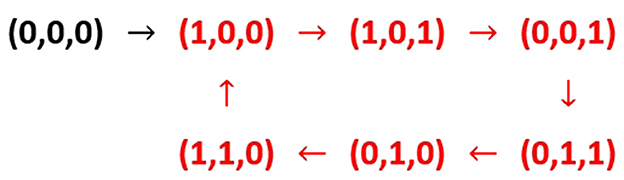
Figure 2. State vector representation of the sequence of neuronal activation leading to Tritonia swimming. Each parenthesis contains the state-dependent “on” (1) or “off” (0) values characterizing the activity or rest of (ID, IV, C2). The arrows indicate the activation sequence, which repeats for several cycles once initiated. The dicycle of the network is shown in red; see Section 10.6.

9 Construction of the transfer function F

We are now ready to build the Boolean function F: ${\mathbb{Z}}_2^3\to {\mathbb{Z}}_2^3$, which in this case is defined as F = (f_DI, f_VI, f_C2), and its logical digraph. We must remember that F^t represents the state of the network at time t, therefore for a sufficiently large t (t ≥ 8, in this example), the biological system will transit around the entire dicycle [20–23].

We will start by defining:

1. $\mathcal{G}=${ID, VI, C2}

and

2. $\mathcal{S}$ = {(0,0,0), (1,0,0), (1,0,1), (0,0,1), (0,1,1), (0,1,0), (1,1,0)},

which is the set of state vectors representing the different sequential working states.

Recall that η is obtained by applying the transfer function F to each vector of ${\mathbb{Z}}_2^n,$and that there is a unique arrow from v to F(v), for every $v\in {\mathbb{Z}}_2^n.$ Therefore,

3. From the network η, we know that:

F(0, 0, 0) = (f_DI(0, 0, 0), f_VI(0, 0, 0), f_C2(0, 0, 0)) = (1, 0, 0), F(1, 0, 0) = (1, 0, 1), F(1, 0, 1) = (0, 0, 1), F(0, 0, 1) = (0, 1, 1), F(0, 1, 1) = (0, 1, 0), F(0, 1, 0) = (1, 1, 0) and F(1, 1, 0) = (1, 0, 0).

where,

f_DI(0, 0, 0) =1,

f_VI(0, 0, 0) = 0,

f_C2(0, 0, 0) = 0.

The same procedure must be repeated for every state vector of the system.

To build explicitly the Boolean function f_DI: ${\mathbb{Z}}_2^3\to {\mathbb{Z}}_2$ we have to find all the state-vectors of $\mathcal{S}$ that under f_DI are going to give 1. They are (0,0,0), (1,0,0), (0,1,0) and (1,1,0).

By using bijection, we have:

$\begin{array}{l}{f}_{DI}(a_{DI},a_{VI},a_{C2})\\ ={\displaystyle \underset{\begin{array}{l}v\in {\mathbb{Z}}_2^n\\ f_{DI}\left(v\right)=1\end{array}}{\oplus }}({\displaystyle \underset{\begin{array}{l}j\in \{DI,VI,C2\}\\ v_j=1\end{array}}{\otimes }}{a}_j)\otimes ({\displaystyle \underset{\begin{array}{l}j\in \{DI,VI,C2\}\\ v_j=0\end{array}}{\otimes }}\left(1\oplus a_j\right)) =\\ ={\displaystyle \underset{v\in \{\left(0,0,0\right),\left(1,0,0\right),\left(0,1,0\right),\left(1,1,0\right)\}}{\oplus }}({\displaystyle \underset{\begin{array}{l}j\in \{DI,VI,C2\}\\ v_j=1\end{array}}{\otimes }}{a}_j)\otimes \\ ({\displaystyle \underset{\begin{array}{l}j\in \{DI,VI,C2\}\\ v_j=0\end{array}}{\otimes }}\left(1\oplus a_j\right)) =\\ =[\left(1\oplus a_{DI}\right)\otimes \left(1\oplus a_{VI}\right)\otimes \left(1\oplus a_{C2}\right)]\oplus [a_{DI}\otimes \left(1\oplus a_{VI}\right)\\ \otimes \left(1\oplus a_{C2}\right)]\oplus [\left(1\oplus a_{DI}\right)\otimes a_{VI}\otimes \left(1\oplus a_{C2}\right)]\\ \oplus [a_{DI}\otimes a_{VI}\otimes \left(1\oplus a_{C2} \right)]\end{array}$

And by utilizing the known equalities

a ⊗ a = a

a ⊕ a = 0

a⊕(a⊕1) = 1

a⊗(a⊕1) = 0,

we get that f_DI(a_DI, a_VI, a_C2) = (1⊕ a_C2) ⊗1. The constant function 1 equals the tautology that represents the excitatory autapse in Figure 1.

To build f_VI, we repeat the procedure. The state vectors with a 1 value under f_VI are (0,0,1), (0,1,1) and (0,1,0). Then,

$\begin{array}{l}{f}_{VI}(a_{DI},a_{VI},a_{C2})=\\ {\displaystyle \underset{\begin{array}{c}v\in \left(0,0,1\right),\left(0,1,1\right),\left(0,1,0\right)\}\end{array}}{\oplus }}({\displaystyle \underset{\begin{array}{c}j\in \{DI,VI,C2\}{v}_j=1\end{array}}{\otimes }}{a}_j)\otimes \\ ({\displaystyle \underset{\begin{array}{c}\begin{array}{l}j\in \{DI,VI,C2\}\\ v_j=0\end{array}\end{array}}{\otimes }}\left(1\oplus a_j \right))=\\ =[\left(1\oplus a_{DI}\right)\otimes \left(1\oplus a_{VI}\right)\otimes a_{C2}]\oplus [\left(1\oplus a_{DI}\right)\otimes a_{VI}\otimes a_{C2}]\\ \oplus [\left(1\oplus a_{DI}\right)\otimes a_{VI}\otimes \left(1\oplus a_{C2} \right)]=\\ =(a_{DI}\oplus 1)\otimes [(a_{VI}\otimes a_{C2})\oplus a_{VI}\oplus a_{C2}]\oplus 1.\end{array}$

Likewise,

$\begin{array}{l}{f}_{C2}(a_{DI}{,a}_{VI}{,a}_{C2})=\\ {\displaystyle {\displaystyle \underset{\begin{array}{c}v\in \left\{(1,0,0),(1,0,1),(0,0,1)\right\}\end{array}}{\oplus }}}({\displaystyle {\displaystyle \underset{\begin{array}{c}j\in \left\{DI,VI,C2\right\}\\ v_j=1\end{array}}{\otimes }}}{a}_j)\otimes \\ ({\displaystyle {\displaystyle \underset{\begin{array}{c}j\in \left\{DI,VI,C2\right\}\\ v_j=0\end{array}}{\otimes }}}(1\oplus a_j))=\\ =\left[(a_{DI}\otimes a_{C2})\oplus a_{DI}\oplus a_{C2}\right]\otimes (a_{VI}\oplus 1)\\ =\left[(a_{DI}\otimes a_{C2})\oplus a_{DI}\oplus a_{C2}\right]\otimes (a_{VI}\oplus 1).\end{array}$

Therefore,

$\begin{array}{l}F(a_{DI},a_{VI},a_{C2})=\\ ((1\oplus a_{C2})\otimes 1,(a_{DI}\oplus 1)\otimes [(a_{VI}\otimes a_{C2})\oplus a_{VI}\oplus a_{C2}]\otimes 1,\\ (a_{DI}\otimes a_{C2})\oplus a_{DI}\oplus a_{C2}]\otimes (a_{VI} \oplus 1)).\end{array}$

Again, let's take f_DI(a_DI, a_VI, a_C2) = (1⊕ a_C2) ⊕1 to find the logical connectives in DI. Table 2 shows that the logical proposition corresponding to 1⊕ a_C2 is “NOT(C2)”, which corresponds to:

Let's now repeat the analysis for VI:

f_VI(a_DI, a_VI, a_C2) =(a_DI ⊕ 1) ⊗ [(a_VI ⊗ a_C2) ⊕ a_VI ⊕ a_C2]

with the corresponding logical proposition “NOT(DI) AND (VI OR C2)”. From Table 2, we obtain the logical digraph in VI:

Finally, we obtain C2:

f_C2(a_DI, a_VI, a_C2) =[(a_DI ⊗ a_C2) ⊕ a_DI ⊕ a_C2] ⊗ (a_VI ⊕ 1),

whose logical proposition is “(DI OR C2) AND NOT(VI)”, and its logical digraph is:

The assembly of all the components above illustrates the logical diagram of the neural regulatory network involved in Tritonia swimming, as shown in Figure 3.

Figure 3

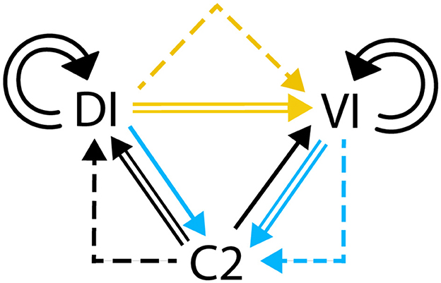
Figure 3. Digraph describing the neural network of Tritonia swimming.

Note that a benefit of the composition of connectives in the logical digraph, is the possibility to analyze subcompartments of the network. For example, the interactions from a to b and from b to c provide the interaction from a to c. Therefore, D1 C2 and are equivalent representations of DI to C2.

Another observation concerns the equivalence of logical propositions in Section 1.1. The effect of autapses, shown as tautologies in Figure 3, enhances the firing of VI and DI neurons. The functioning of the regulatory network could be simplified by removing the tautologies that represent these connections. However, we recommend including all components that contribute to a more accurate representation of the circuit dynamics.

The digraph in Figure 3 contrasts with the excitation-inhibition graph in Figure 1A, which not replicate the functional network.

10 Dynamics of the network

In the first part of our paper, we went from the transfer function F: $\mathcal{S}\to \mathcal{S}$ of a biological system to its logical digraph. In this section, we will discuss the tools for studying the dynamics of a regulatory network of a biological system.

10.1 Sketch

This section will describe the connected components of η and the dynamics of the biological system by utilizing the transfer function F, its orbits, and the state matrix M_η of the regulatory network η.

Section 10.2 provides essential definitions to comprehend the network topology and the flow of information between F and η.

Section 10.3 outlines the basic properties of the transfer function F.

Section 10.4, defines the properties of the state-matrix M_η and its spectrum, composed of the eigenvectors and eigenvalues of M_η. The Spectrum provides us with additional tools to study the dynamics of the regulatory network η.

Section 10.5 illustrates how to translate information between the transfer function F and the state-matrix M_η. This transfer of information will assist us in retrieving the Boolean information of the network as we study its dynamics over time.

Section 10.6 shows that network η is a digraph, that is, a graph that instead of edges has arrows (see Figures 2, 4 and the glossary). η may be connected, as shown in the network in Figure 2, or it may not be connected, as illustrated in Figure 4, where η has two connected components. C₁ and C₂. It is important to determine whether the network η is connected, as each connected component contains different biological information. We will need to construct and analyze each connected component separately to prevent information overlap that could lead to inaccurate results.

Figure 4

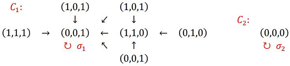
Figure 4. Regulatory network of Tritonia swimming based on pure excitation and inhibition connectives. The network has two connected components C₁ and C₂. The loop σ₁ in (0,0,1) is the attractor of C₁, while the loop σ₂ in (0,0,0) is the attractor of C₂ (see also Sections 10.2 and 10.6).

The Supplementary material 1 contains computer programs designed to determine which components are connected in η. The Supplementary material 2 includes a computer program intended to obtain the transfer function F from the regulatory network η.

10.2 Topology of network dynamics

Let us begin this second part by introducing some necessary definitions for analyzing network dynamics. For further assistance, the glossary contains definitions of the terms presented in this study. Figure 5 illustrates the essential configurations of a network. A simple case arises when one element connects to itself, forming a loop known as an attractor (Figure 5A). Mathematically, an attractor v is a fixed point of F. Therefore, F(v)=v. The network in Figure 4 has two attractors, one at the state vector (0,0,1) and another at the state vector (0,0,0).

Figure 5

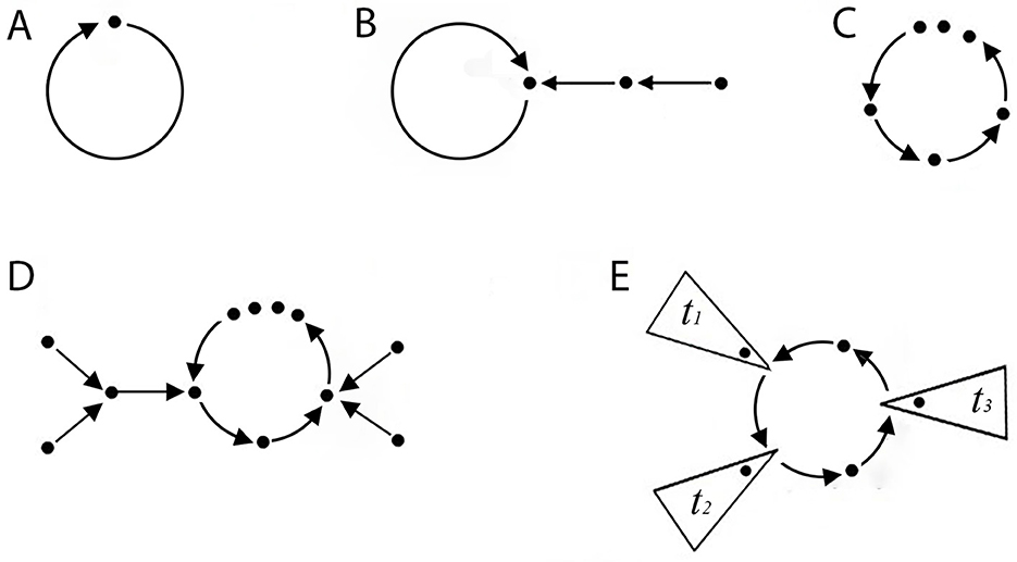
Figure 5. Elementary shapes of a connected network η. Each paragraph describes a connected network (digraph). The dots represent elements, and the arrows denote connections. (A) A single connected element forms a loop (attractor) without ditrees. (B) An attractor with a ditree. (C) Structure of a dicycle (limit cycle). (D) A limit cycle receiving two ditrees (on the right and left sides). (E) A simplified representation of a limit cycle with ditrees labeled as t1, …, tl. Each ditree may contain one or multiple elements.

This result provides a means to count the forms of a connected component with n states. See also [24, 25].

A more complex case shown in Figure 5C arises when a dicycle in η contains multiple elements connected in series, forming a loop. This configuration creates a limit cycle, specifically a closed loop that establishes a stable feedback system. It is important to note that an attractor would be a limit cycle of size 1. Mathematically, there is a set of state-vectors, {v₁, …, v_m} with size m > 1, such that:

$\begin{array}{c}F(v_1)=v_2,\dots ,F(v_{m-1})=v_m\text{ and }F(v_m)=v_1.\end{array}$

The limit cycle in the neural network of Tritonia swimming in Figure 2, contains a peripheral element called ditree (T). Most regulatory networks in biology contain one or more ditrees (Figures 5B, D, E), which establish unidirectional connections to the main loop or dicycle of η. A connected component serves as an input that activates or modulates the dynamics of η. A network that receives ditrees is known as a connected network.

After defining the components of the biological network, including their connectivity and topology, the structure-function relationship can be quantitatively analyzed by examining the information flow between F and η. Figure 6 summarizes the basis of this information flow.

Figure 6

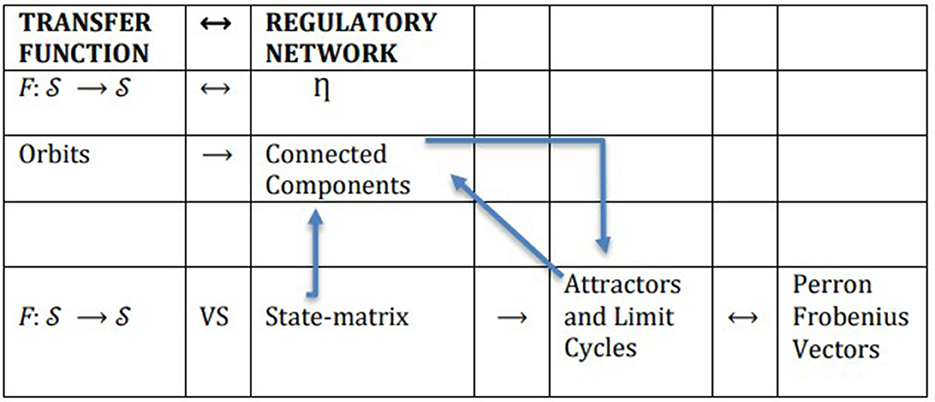
Figure 6. Information flow between F and η.

Mathematically, a connected component of a network η is a maximal connected subgraph of its underlying graph |η|. For instance, the network in Figure 4 has two connected components: C1 and C2. In contrast, the network in Figure 2 is a connected network. (For definitions and results of graph theory, see Chartrand et al. [20]). It should be noted that theoretically, η may be “not connected,” although most biological cases are connected networks with multiple inputs and regulatory elements.

10.3 The transfer function F and its orbits

The regulatory network is constructed employing a set-function F: $\mathcal{S}$→$\mathcal{S}$ that we will refer to as the transfer function F and its compositions, as follows:

Let us recall that $\mathcal{S}$ refers to the set of state vectors of the biological system comprising n elements (genes, cells, etc.). Time plays a crucial role in the development of this work. Thus, we can now assign a time-dependence to the evolution of the network as follows: F⁰ = $I_{\mathcal{S}}$ is the identity function of $\mathcal{S}$, F¹ = F, and for each time t > 1, F ^t =F∘F∘⋯∘ F denotes t times its composition. That is:

F ^t (v)= F ^t−1 (F(v)).

10.3.1 Shape of the digraph of a function

Since F is a set-function, for each v in $\mathcal{S}$, there is a unique w such that v is sent under F to w, as denoted by F(v) = w. This property permits the connected components of the network to acquire some of the shapes described in Figure 5. From each element v in $\mathcal{S}$ emerges one unique arrow to F(v). However, any element of $\mathcal{S}$ may receive two or more arrows.

10.3.2 Connected components and unique cycles

Every connected component of η has a unique dicycle. The network η defined by F has as vertices the elements of $\mathcal{S}$ and arrows vη F(v), for each v in $\mathcal{S}.$

The transfer function F: $\mathcal{S}$→$\mathcal{S}$ is a set-function. Therefore, all its compositions F^t are also set-functions from $\mathcal{S}$ to $\mathcal{S}$. Since $\mathcal{S}$ is a finite set with s elements, for each v in $\mathcal{S}$, the set {F^t(v): t ≥ 0}, which is a subset of $\mathcal{S},$ has at most s elements. Therefore, there exists 0 ≤ m<t ≤ s such that F^m(v)= F^t(v). This means that, F^m(v) → F^m+1(v) → ⋯ → F^t(v)= F^m(v) is a dicycle. According to Section 10.3.1, this dicycle is unique.

10.3.3 Orbits of the transfer function

We will now define the orbit of a state vector v, whose interest lies in containing information about the evolution of the dynamics of the network. Mathematically, the orbit of v in $\mathcal{S}$ is the set {F ^t(v): t ≥ 0} and will be denoted by Ω(v). According to Sections 10.3.1 and 10.3.2, Ω(v) contains a unique dicycle.

An example of topology with orbits and a ditree can be found in the regulatory network of Tritonia swimming (Figure 7), which includes two different orbits, one of which incorporates all the elements:

Figure 7

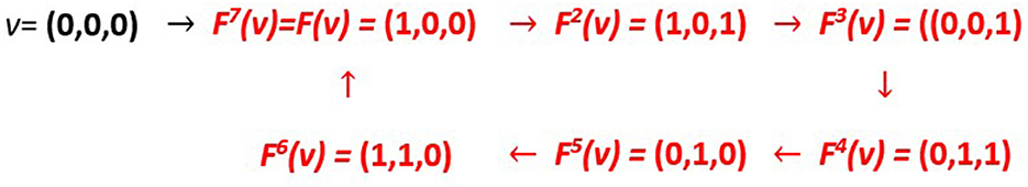
Figure 7. The network of Tritonia swimming has an orbit that incorporates all the elements Ω(v) = {(0,0,0), (1,0,0), (1,0,1), (0,0,1), (0,1,1), (0,1,0), (1,1,0)} while the other orbit (red) is the limit cycle of the network.

Ω(v) = {(0,0,0), (1,0,0), (1,0,1), (0,0,1), (0,1,1), (0,1,0), (1,1,0)} with v=(0,0,0).

The other orbit is the limit cycle of the network (red in Figure 7):

{(1,0,0), (1,0,1), (0,0,1), (0,1,1), (0,1,1), (0,1,0), (1,1,0)}

= Ω((1,0,0))= Ω((1,0,1))= Ω((0,0,1))= Ω((0,1,1))= Ω((0,1,0))= Ω((1,1,0)).

10.3.4 Shape of the connected components

Since each orbit has a unique dicycle (as seen in Section 10.3.3), any additional arrow serves as a ditree pointing to the dicycle. Figure 5 illustrates the general shape of the connected components of a regulatory network; Sections 10.6 and 10.7 present a method for constructing them. A computer routine for the same purpose is included in a Supplementary file.

10.4 The state-matrix of η and its spectral properties

Now we will define the state matrix, denoted by Mη, which not only stores information about the transition function (see Section 10.3) but also provides the temporal dynamics of the biological system.

To define M_η we must first fix an order in $\mathcal{S}=\left\{v_1,\dots ,v_s\right\}$. M_η is a real matrix of size s × s, whose ij-th entry is:

$\begin{array}{c}{M}_{\eta }(i,j)=\{\begin{array}{cc}1& {ifv}_j\to v_i\text{ is an arrow in }\eta \\ 0& \text{otherwise}\end{array}\end{array}$

Any order conveys equivalent biological information since the corresponding state matrices are conjugated.

Observe that $M_{\eta }+M_{\eta }^T$ (where $M_{\eta }^T$ denotes the transpose matrix of M_η) is the adjacency matrix of the underlying graph of η. As an example, we can now define the M_η of the Tritonia swimming regulatory network η (see Section 10.3.3 or Figure 2) as:

$\begin{array}{l}S=\{v_1=\left(1,0,0\right),v_2=\left(1,0,1\right),v_3=\left(0,0,1\right),v_4=\left(0,1,1\right),\\ v_5=\left(0,1,0\right),v_6=\left(1,1,0\right),v_7=\left(0,0,0 \right)\}.\end{array}$

With such order, the state-matrix M_η of the network is:

$\begin{array}{c}{M}_{\eta }=\left[\begin{array}{c}0000011\\ 1000000\\ 0100000\\ 0010000\\ 0001000\\ 0000100\\ 0000000\end{array}\right]\end{array}$

with eigenvector $\left(\begin{array}{c}\begin{array}{c}1\\ ⋮\\ 1\end{array}\\ 0\end{array}\right)$ of the eigenvalue 1

10.5 Spectrum of M_η

The characteristic polynomial of M_η gives the number of connected components of η. Furthermore, the Perron-Frobenius eigenvectors reveal the attractors and limit cycles. We will now demonstrate that the characteristic polynomials of the state matrices for the dicycles and ditrees completely characterize the characteristic polynomial and the spectrum of the state matrix.

10.5.1 Polinomial of the state matrix of a dicycle

The characteristic polynomial p_σ(x) of a dicycle σ of size r, is:

$\begin{array}{c}{p}_{\sigma }(x)={\prod }_{k=1}^r(x{-e}^{\frac{2\pi ki}{r}}),\end{array}$

where $\left\{e^{\frac{2\pi ki}{r}};k=1,\dots ,r\right\}$ are the r-roots of unity, defined as the complex numbers z, such that z^r=1, and e^2πi = 1 (see Chartrand et al. [20]).

The above result is established, and it is also recognized that the state matrix of a dicycle σ is as follows:

$\begin{array}{c}{M}_{\sigma }=\left[\begin{array}{c}0000001\\ 1000000\\ 0100000\\ 0010000\\ 0001000\\ 0000100\\ 0000010\end{array}\right]\end{array}$

with eigenvector $\left(\begin{array}{c}1\\ ⋮\\ 1\end{array}\right)$ of the eigenvalue 1

10.5.2 Characteristic polinomial of a ditreee

The characteristic polynomial of a ditree T of size q, is p_T(x)= x^q (see Chartrand et al. [20]). By convention (see Section 10.3.3), a ditree T of η has a size bigger than 1 and contains a unique vertex in the dicycle of η (see Figure 7).

10.5.3 Polynomial of the state matrix of the network

Now we can analyze the characteristic polynomial of M_η when the regulatory network η is connected. Recall that the vertices of η are the elements of $\mathcal{S}=\left\{v_1,\dots ,v_s\right\}$ and that η has a unique dicycle σ of size r and possibly, T₁, ..., T_d ditrees with d≥ 0 and each T_h of size q_h. Then the characteristic polynomial of M_η is:

$\begin{array}{c}{p}_{M_{\eta }}(x)=p_{\sigma }(x){\prod }_{h=1}^d{p}_{T_h}(x)={\prod }_{k=1}^r(x-e^{\frac{2\pi ki}{r}})x^{(\sum _{h=1}^d{q}_h)-d}.\end{array}$

In this case, 1 is an eigenvalue of M_η with a unique (up to scalar multiples) eigenvector $\widehat{u}$ = (u₁,…, u_s), where u_i =1 if v_i belongs to the dicycle, and u_i =0 otherwise. Since all the eigenvalues have modulus equal to r ≤ 1 (and 1 is also an eigenvalue of M_η), the maximum of the modulus of these eigenvalues is 1. This maximum is known as the spectral radius (ϱ_Mη) of M_η and is denoted by:

$\begin{array}{c}{\varrho }_{M_N}=max\left\{\left|\right|\lambda \left|\right|,with\lambda beingeigenvalueofM\right\}\end{array}$

The eigenvector $\widehat{u}$ of ϱ_Mη is the Perron-Frobenius (eigen)vector of M_η and gives us a way to find the vertices of η, which form its attractor or limit cycle, as will be shown in Section 10.6.

10.5.4 The generation of Mη

If η is not connected, we can define an order of $\mathcal{S}$ such that M_η has the following form:

$\begin{array}{c}{M}_{\eta }=\left[\begin{array}{cccc}{M}_{{\mathcal{C}}_1}& 0& & 0\\ 0& M_{{\mathcal{C}}_2}& & 0\\ & & \ddots & \\ 0& 0& & M_{{\mathcal{C}}_m}\end{array}\right]\end{array}$

with ${\mathcal{C}}_1,...,{\mathcal{C}}_m$ being the different connected components of η and their respective state-matrices being $M_{{\mathcal{C}}_1}$,…, $M_{{\mathcal{C}}_m}$(see Section 10.2). Then, the characteristic polynomial of M_η is:

$\begin{array}{c}{p}_{M_{\eta }}(x)={\prod }_{j=1}^m{p}_{{\mathcal{C}}_j}(x)\end{array}$

Since ${\mathcal{C}}_j$ is a connected network, $p_{{\mathcal{C}}_j}$(x) has the form described in Section 10.5.3. Therefore, p_Mη(x) = (x-1)^m(x-λ_m+1)...(x-λ_s), with λ_m+1,…, λ_s ≠ 1. In other words, the maximum power of x − 1 in the characteristic polynomial of M_η indicates the number of connected components of η. Section 10.7 contains an algorithm to find such components.

For example, we can now refer to the network in Figure 4. Its characteristic polynomial is x⁸ − 2x⁷ + x⁶ = x⁶(x − 1)². The power of x-1 is 2. Therefore, as shown in Figure 4, η has two connected components.

10.5.5 The transfer function vs. the state-matrix

To gain further insight about the regulatory network, it will be useful to analyze the relationship between the transfer function $F:\mathcal{S}\to \mathcal{S}$ and the state-matrix M_η, as they collectively store information about network dynamics. In brief, F informs about the individual state vectors, and M_η gives the “global connectivity” of each state vector.

Let s be the number of elements of $\mathcal{S}$, and recall that for each t ≥ 0, F⁰= $I_{\mathcal{S}}$, F¹ = F and $F^t=F$∘ . . .∘F t times the composition of F, and M_η is a real matrix of size s × s (see Section 10.3).

For each subindex i = 1, …, s, denoted by e_i is the real column-vector that has 1 in the i-th coordinate and 0 elsewhere. Now we have two types of bijective set functions.

The first bijection occurs between the set of state-vectors $\mathcal{S}$ and the collection of vectors {e₁, …, e_s }:

$\begin{array}{c}\begin{array}{c}\mathcal{S}\rightleftarrows \left\{e_1,\dots ,e_s\right\}\\ v_i\rightleftarrows e_i\end{array}\end{array}$

Recall that any real vector is a linear combination of the vectors e₁, …, e_s. Therefore, to study the state-matrix M_η it is enough to study the image of these vectors under M_η.

The second type of bijection is established between the orbit of v_i under F, {$F^t{v}_i:t\ge 0$}, and the orbit of e_i under the matrix M_η, {$M_{\eta }^t{e}_i:t\ge 0$}. Recall that any real vector is a linear combination of the vectors e₁, …, e_s. Therefore, for each state vector v_i, we have one bijection:

$\begin{array}{c}\begin{array}{c}\left\{F^t{v}_i:t\ge 0\right\}\rightleftarrows \left\{M_{\eta }^t{e}_i:t\ge 0\right\}\\ F^t{v}_i\rightleftarrows M_{\eta }^t{e}_i\end{array}\end{array}$

10.6 The connected components of the network η

We can now discuss a method for finding the connected components of η. As mentioned earlier, each connected component must be studied separately to prevent mixing information that could lead to false results.

10.6.1 Number of connected components of η

As described in Section 10.5.4, the characteristic polynomial of M_η is p_Mη(x) = (x-1)^m(x-λ_m+1)...(x-λ_s), where λ_m+1,…, λ_s are different from 1. Therefore, η has m different connected components. Moreover, the non-zero entries of the eigenvectors associated with the eigenvalue 1 are the vertices of the attractors and limits cycles of η.

Following the example in Figure 4 and (Section 10.5.4), the vertices of η are:

v₁=(0,1,0), v₂=(0,0,0), v₃=(1,0,0), v₄=(1,1,1), v₅=(0,1,1), v₆=(1,0,1), v₇=(1,1,0) and v₈=(0,0,1).

The characteristic polynomial of M_η is p_Mη(x) = x⁶(x-1)², with the power of x-1 being 2. Therefore, η has two connected components. The eigenvectors of 1 that give the vertices in attractors and limit cycles are (0,1,0,0,0,0,0,1)^T and (0,0,0,0,0,0,0,1)^T, with their non-zero entries corresponding to the state-vectors v₂ and v₈. To get the attractors and limit cycles we calculate their orbits Ω(v₂) = {v₂} and Ω(v₈) = {v₈}. Therefore, η has exactly two attractors, one in v₂ = (0,0,0) and the other in v₈ =(0,0,1), as we can confirm in Figure 4.

10.6.2 Vertices of the connected components of η

With the attractors and limit cycles of the network η, we need to identify the vertices in the connected components they define. Using orbits again, if a vertex v is in a connected component C, the complete orbit Ω(v) is contained in C and Ω(v) contains the dicycle of C. Therefore, two state vectors belong to the same connected component if their orbits have a non-empty intersection. Moreover, they must share the same dicycle.

Following the example in Figure 4 and Section 10.2, we get that the vertices v₁= (0,1,0), v₃= (1,0,0), v₄= (1,1,1), v₅= (0,1,1), v₆= (1,0,1), v₇= (1,1,0), and v₈=(0,0,1) form a connected component, while the other connected component is a loop in v₂= (0,0,0), as one can verify in Section 10.5.4.

10.7 An algorithm to construct the connected components of η

We can now reconstruct the dynamics of the network using the following cookbook, which can be algorithmized at every step:

1. Obtain M_η using any order of $\mathcal{S}$.

2. η has m different connected components, where m is the maximal power of x-1 in the characteristic polynomial p_Mη(x). That is:

p_Mη(x)=(x-1)^m (x -λ_m+1)...(x-λ_s), with λ_m+1,…, λ_s different from 1.

The set of vertices corresponding to the non-zero coordinates of the eigenvectors associated with eigenvalue 1 forms the vertices of the dicycles of η.

Now select one of those vertices, say v, then the orbit Ω(v) must be the attractor or limit cycle of a connected component of the network η.

3. Now we will build each connected component.

Assuming that m different dicycles (say σ₁, …, σ_m) correspond to m different connected components, we must now find their state vectors. According to Section 10.6.2, two state vectors belong to the same connected component if their orbits intersect non-empty.

10.8 Topology of the network

By demonstrating that each connected component of η has exactly one attractor or limit cycle designated by the Perron-Frobenius eigenvector of the network's state matrix, this section provides mathematical evidence showing how attractors and limit cycles illustrate the temporal dynamics of the biological system. The technique is described in Figures 1, 2, 7 of the Tritonia regulatory network section. The Perron-Frobenius Theorem shows that these attractors and limit cycles define the “phenotype” of the biological system. In other words, if v is the state vector of one connected component, η′ of η and M', the defined state matrix η′, then the evolution of v in time m, given by (M')^mv, tends to the attractor or limit cycle of evolution η′. Moreover, each connected component of the network can be analyzed as a separate biological subsystem, independently of those describing other connected components (see Section 10.3).

In summary, the regulatory network of a synchronous biological system may include different connected components, each representing an independent subsystem. Therefore, we should evaluate each component separately. This reflects the nature of a connected regulatory biological network. As shown above, such networks have a single attractor or limit cycle. According to the Perron-Frobenius theorem, the attractor reflects the system's time-dependent behavior. By definition, this attractor is stable.

10.8.1 The regulatory network of Tritonia

The regulatory network η of Tritonia swimming is a connected network with the following seven state vectors:

$\begin{array}{l}{v}_1=(1,0,0),v_2=(1,0,1),v_3=(0,0,1),v_4=(0,1,1),\\ v_5=(0,1,0),v_6=(1,1,0).\end{array}$

The 7 by 7 state matrix and its eigenvector u with eigenvalue 1 have been presented in section 10.6.1. In Figure 8 note that η has a unique ditree v₇ → v₁ with v₇ = (0,0,0). The ij-th entry of M_η occurs into the ith row and the jth column, and acquires a 1 value if there is an arrow in η from v_j to v_i.

Figure 8

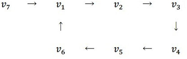
Figure 8. Structure of the regulatory network of Tritonia Swimming, displaying a unique ditree v₇ → v₁.

As described in Section 10.5, the ith entry corresponds to the state-vector v_i, which has a value of 1, indicating that it is at limit cycle. Moreover, 1 is the spectral radius of M_η and its eigenvector is the Perron-Frobenius vector of the state-matrix.

As we will see in Section 10.5, for certain matrices such as M_η, if η is a connected network, the Perron-Frobenius vector, u, acquires the following asymptotic property:

$\begin{array}{c}{\displaystyle \underset{m\to \infty }{lim}}{M}_{\eta }^{m}v={\alpha }_{v}uwith{\alpha }_v>0\end{array}$

For every v in K = {$\sum _{i=1}^7{a}_i{z}_i:a_i\ge 0$for i=1,…,7}. This set K is built with the orbits of the state-vectors of the network defined in Sections 10.3.3 and 10.5.5. For Tritonia swimming, the vectors z_i are the following:

z₁= (0,1,1,1,1,1,0) vector associated to the orbit v₁.

z₂= (1,0,1,1,1,1,0) vector associated to the orbit v₂.

z₃= (1,1,0,1,1,1,0) vector associated to the orbit v₃.

z₄= (1,1,1,0,1,1,0) vector associated to the orbit v₄.

z₅= (1,1,1,1,0,1,0) vector associated to the orbit v₅.

z₆= (1,1,1,1,1,0,0) vector associated to the orbit v₆.

z₇= (1,0,0,0,0,0,1) vector associated to the orbit v₇.

Figure 9 illustrates the meaning of the limit just described.

Figure 9

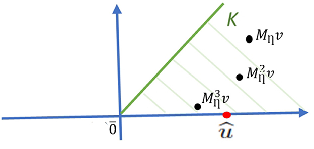
Figure 9. Geometric interpretation of the Birkhoff-Vandergraft theorem. The non-negativity of the M_η matrix allows the use of the Perron-Frobenius theorem described in Section 10.8.4. û is the Perron-Frobenius vector; K is the set of real vectors v, and $M_{\eta }^{t}v$ is the state matrix of η for a vector v over time t.

Now, we will contextualize the previous facts.

10.8.2 Perron-Frobenius eigenvector of M_η

According to the Jordan decomposition theorem, the eigenvalues and eigenvectors of a matrix determine the behavior of the linear function defined by the matrix [26–28]. More specifically, the spectral radius of the state-matrix M_η provides an asymptotic prediction of the behavior of the connected network over time (see Section 10.8).

The set K of real vectors is defined by the orbits of the state vectors of η (see Section 10.3.3). K is invariant under the state-matrix M_η, meaning that for every vector v in K, M_ηv also lies in K. Moreover, for t $\ge 0,M_{\eta }^{t}v$ K approaches the ray determined by the Perron-Frobenius eigenvector û, with its unique eigenvalue ρ(M_η) = 1 (see Section 10.5.3). Such ray is the asymptote of $M_{\eta }^{t}v$ which informs about the temporal dynamics of the biological network.

10.8.3 A cone associated to η

To construct the set K, we must remember that the vertices of η are the state vector $\mathcal{S}=\{v_1,\dots ,v_s\}$, with {v₁, …, v_m} being the dicycle or the network. If m=1, {v₁, …, v_m} represents the attractor. Otherwise, {v₁, …, v_m} represents the limit cycle of η.

Now we will define the real vectors in s coordinates. For 1 ≤ i ≤ s, the vector z_i contains the information about the state-vectors in the orbit of the state-vector v_i. In the following equation, the jth-coordinate is:

$\begin{array}{c}{Z}_i\left(j\right)=\{\begin{array}{l}1\text{ if }{v}_j\text{ belongs to the orbit of }{v}_i\hfill \\ 0\text{ otherwise}\hfill \end{array}\end{array}$

Remember that the orbit of v_i is:

$\begin{array}{c}\Omega (v_i)=\left\{F^t(v_i):t\ge 0\right\},\end{array}$

which is the set of compositions of F(v_i) in section 10.5.3.

We can now define K as the set of non-negative linear combinations of z₁, …, z_s.,

$\begin{array}{c}K=\left\{{\sum }_{i=1}^s{a}_i{z}_i:a_i\ge 0\text{ for }i=1,\dots ,s\right\}.\end{array}$

10.8.4 Future behavior of the biological system

We have obtained the following asymptotic result: For every v in K, the following limit exists:

$\begin{array}{c}{\displaystyle \underset{m\to \infty }{lim}}{M}_{\eta }^{m}v={\alpha }_vû\text{ with }{\alpha }_v>0\end{array}$

The above result originates from the Birkhoff-Vandergraft Theorem [27], which generalizes the Perron-Frobenius theorem [25, 26].

In the equation above, û is truly a “limit vector” that predicts the future behavior of the biological system. Moreover, as stated in Section 10.5, the non-zero entries of û correspond to the state-vectors of the limit cycle (the attractor) of the network. The behavior of attractors in asynchronous systems is adequately described in Cessac and Samuelides [12].

10.9 An algorithm to find the attractors and the limit cycles of η

It is easy to identify the attractors and limit cycles of small regulatory systems. However, finding the attractors or limit cycles becomes harder when we don't know if the network is connected. The following algorithm is created to identify the attractors and limit cycles.

1. Find all the connected components of η (see Section 10.9).

2. Let ${\mathcal{C}}_1,...,{\mathcal{C}}_m$ be the different connected components of η and $M_{{\mathcal{C}}_1},...,M_{{\mathcal{C}}_m}$ their respective state-matrices.

3. For each h=1, …, m, calculate an eigenvector of $M_{{\mathcal{C}}_h}$, û^(h) with a 1 eigenvalue. The state-vectors of $\mathcal{S}$, associated with the non-zero coordinates of û^(h) form the limit cycle of ${\mathcal{C}}_h$.

11 Conclusions

1. We introduce a method for detecting and illustrating various interactions among the components that control the operation of regulated biological networks.

2. A logical digraph of the regulatory biological network is built using eight logical connectives from Boolean algebra, which together accurately depict all possible interactions among the network's elements.

3. Rules are provided to convert the components of the network from logical to Boolean representation.

4. The transfer function, its orbits, and the state matrix of the network enable us to identify the topology of the network, including its limit cycles, attractors, and dynamics.

5. The spectrum of the state matrix determines the Perron-Frobenius eigenvalues, which predict the time evolution of the network.

6. An algorithm plus three software routines are provided to find the attractors and limit cycles of biological regulatory systems, to build their state matrix and to find the eigenvectors in systems with a large number of elements.

Data availability statement

The original contributions presented in the study are included in the article/Supplementary material, further inquiries can be directed to the corresponding author.

Author contributions

MT: Writing – original draft, Supervision, Project administration, Formal analysis, Conceptualization, Funding acquisition, Investigation, Writing – review & editing. SB-G: Writing – review & editing, Formal analysis, Software, Investigation, Validation, Methodology. JM-M: Validation, Methodology, Investigation, Formal analysis, Software, Writing – review & editing. GG-L: Writing – review & editing, Formal analysis, Validation, Methodology, Software. FD-M: Validation, Data curation, Project administration, Conceptualization, Investigation, Writing – original draft, Writing – review & editing, Funding acquisition, Formal analysis.

Funding

The author(s) declare that financial support was received for the research and/or publication of this article. This study was funded by a grant AG200823 from the Dirección General de Asuntos del Personal Académico, of Universidad Nacional Autónoma de México to FD-M and MT, and by Human Frontiers Science Program Organization RGP0060/2019-102 grants to FD-M.

Acknowledgments

We wish to express our gratitude to Felipe Meneses for his help in obtaining valuable bibliographical material, to Isabel Takane for the typography of the article, and to Francisco Pérez Eugenio for continuously supporting our computer requirements.

Conflict of interest

The authors declare that the research was conducted in the absence of any commercial or financial relationships that could be construed as a potential conflict of interest.

The author(s) declared that they were an editorial board member of Frontiers, at the time of submission. This had no impact on the peer review process and the final decision.

Generative AI statement

The author(s) declare that no Gen AI was used in the creation of this manuscript.

Any alternative text (alt text) provided alongside figures in this article has been generated by Frontiers with the support of artificial intelligence and reasonable efforts have been made to ensure accuracy, including review by the authors wherever possible. If you identify any issues, please contact us.

Publisher's note

All claims expressed in this article are solely those of the authors and do not necessarily represent those of their affiliated organizations, or those of the publisher, the editors and the reviewers. Any product that may be evaluated in this article, or claim that may be made by its manufacturer, is not guaranteed or endorsed by the publisher.

Supplementary material

The Supplementary Material for this article can be found online at: https://www.frontiersin.org/articles/10.3389/fams.2025.1644869/full#supplementary-material

References

1. Getting PA. Tritonia swimming: triggering of a fixed action pattern. Brain Res. (1975) 96:128–33. doi: 10.1016/0006-8993(75)90584-3

PubMed Abstract | Crossref Full Text | Google Scholar

2. Álvarez-Buylla E, Benítez M, Corvera-Poiré A, Chaos Cador A, de Folter S, Gamboa de Buen A, et al. Flower development. The Arabidopsis Book (2010) 8:e0127. doi: 10.1199/tab.0127

PubMed Abstract | Crossref Full Text | Google Scholar

3. Chaos A, Aldana M, Espinosa-Soto C, García B, Garay A, Alvarez-Buylla E. From genes to flower patterns and evolution: dynamic models of gene regulatory networks. J Plant Growth Regul. (2006) 25:278–89. doi: 10.1007/s00344-006-0068-8

Crossref Full Text | Google Scholar

4. Cortes-Poza Y, Padilla-Longoria P, Alvarez-Buylla E. Spatial dynamics of floral organ formation. J Theor Biol. (2018) 454:30–40. doi: 10.1016/j.jtbi.2018.05.032

PubMed Abstract | Crossref Full Text | Google Scholar

5. Schwab JD, Kühlwein SD, Ikonomi N, Kühl M, Kestler HA. Concepts in Boolean network modeling: what do they all mean? Comput Struct Biotechnol J. (2020) 18:571–82. doi: 10.1016/j.csbj.2020.03.001

PubMed Abstract | Crossref Full Text | Google Scholar

6. Baths V, Roy U, Singh T. Disruption of cell wall fatty acid biosynthesis in Mycobacterium tuberculosis using a graph theoretic approach. Theoret Biol Med Modell. (2011) 8:5. doi: 10.1186/1742-4682-8-5

PubMed Abstract | Crossref Full Text | Google Scholar

7. Moore MN, Shaw JP, Ferrar Adams DR, Viarengo A. Anti-oxidative cellular protection effect of fasting-induced autophagy as a mechanism for hormesis. Mar Environ Res. (2015) 107:35–44. doi: 10.1016/j.marenvres.2015.04.001

PubMed Abstract | Crossref Full Text | Google Scholar

8. Wang Y, Liu X, Dong L, Cheng K-K, Lin C, Wang X, et al. iMSEA: a novel metabolite set enrichment analysis strategy to decipher drug interactions. Anal Chem. (2023) 95:6203–11. doi: 10.1021/acs.analchem.2c04603

PubMed Abstract | Crossref Full Text | Google Scholar

9. Palma E, Salinas L, Aracena J. Enumeration and extension of non-equivalent deterministic update schedules in Boolean networks. Bioinformatics. (2016) 32:722–9. doi: 10.1093/bioinformatics/btv628

PubMed Abstract | Crossref Full Text | Google Scholar

10. Kauffman SA. The Origins of Order. Self-Organization and Selection in Evolution. New York, NY: Oxford University Press (1993). doi: 10.1093/oso/9780195079517.001.0001

Crossref Full Text | Google Scholar

11. Giacomantonio CE, Goodhill GJ. A boolean model of the gene regulatory network underlying mammalian cortical area development. PLoS Comput Biol. (2010) 6:e1000936. doi: 10.1371/journal.pcbi.1000936

PubMed Abstract | Crossref Full Text | Google Scholar

12. Cessac B, Samuelides M. From neuron to neural networks dynamics. Eur Phys J Special Topics. (2007) 142:7–88. doi: 10.1140/epjst/e2007-00058-2

Crossref Full Text | Google Scholar

13. Getting PA. Mechanisms of pattern generation underlying swimming in Tritonia III. Intrinsic and synaptic mechanisms for delayed excitation. J Neurophysiol. (1983) 49:1036–50.

PubMed Abstract | Google Scholar

14. Kleinfeld D, Sompolinsky H. Associative neural network model for the generation of temporal patterns. Theory and application to central pattern generators. Biophysical J. (1988) 54:1039–51. doi: 10.1016/S0006-3495(88)83041-8

PubMed Abstract | Crossref Full Text | Google Scholar

15. Getting PA. Mechanisms of pattern generation underlying swimming in Tritonia IV. Gating of central pattern generator. J Neurophysiol. (1985) 53:466–80. doi: 10.1152/jn.1985.53.2.466

PubMed Abstract | Crossref Full Text | Google Scholar

16. Dorsett DA, Willows OD, Hoyle G. The neuronal basis behavior in Tritonia IV. The central origin of a fixed action pattern demonstrated in the isolated brain. J Neurobiol. 4:189–300. (1973). doi: 10.1002/neu.480040309

PubMed Abstract | Crossref Full Text | Google Scholar

17. Willows OD, Hoyle G. Neuronal network triggering a fixed action pattern. Science. (1969) 166:1549–51. doi: 10.1126/science.166.3912.1549

PubMed Abstract | Crossref Full Text | Google Scholar

18. Tamvacakis AN, Lillvis JL, Sakurai A, Katz PS. The consistency of gastropod identified neurons distinguishes intra-individual variability in neural circuits. Front Behav Neurosci. (2022) 16:855235. doi: 10.3389/fnbeh.2022.855235

PubMed Abstract | Crossref Full Text | Google Scholar

19. Getting PA. Mechanisms of pattern generation underlying swimming in Tritonia. I Neuronal network formed by monosynaptic connections. J Neurophysiol. (1981) 46:65–79. doi: 10.1152/jn.1981.46.1.65

PubMed Abstract | Crossref Full Text | Google Scholar

20. Chartrand G, Lesniak L, Zhang P. Graphs and Digraphs, 5th Edn. Boca Raton; London; New York; NY: CRC Press (2011). doi: 10.1201/b14892

Crossref Full Text | Google Scholar

21. Cori R, Lascar D. Mathematical Logic: A Course With Exercises. Part I and II. Oxford: Oxford University Press (2000). doi: 10.1093/oso/9780198500490.001.0001

Crossref Full Text | Google Scholar

22. Cunningham DW. Set Theory: A First Course. Cambridge: Cambridge University Press (2016). doi: 10.1017/CBO9781316341346

Crossref Full Text | Google Scholar

23. Schneeweiss WG. Boolean Functions: With Engineering Applications and Computer Programs. Berlin; Heidelberg: Springer Verlag (1989). doi: 10.1007/978-3-642-45638-1

Crossref Full Text | Google Scholar

24. Samuelsson B, Troein C. Superpolynomial Growth in the number of attractors in kauffman networks. Phys Rev Lett. (2003) 90:098701. doi: 10.1103/PhysRevLett.90.098701

PubMed Abstract | Crossref Full Text | Google Scholar

25. Trinh VG, Park KH, Pastva S, Rozum J. Mapping the attractor landscape of Boolean networks with biobalm. Bioinformatics. (2025) 41:btaf280. doi: 10.1093/bioinformatics/btaf280

PubMed Abstract | Crossref Full Text | Google Scholar

26. Horn RA, Johnson CR. Matrix Analysis. Cambridge: Cambridge University Press (1990).

Google Scholar

27. Horn Roger A, Johnson CR. Topics in Matrix Analysis. Cambridge: Cambridge University Press (1999).

Google Scholar

28. Vandergraft JS. Spectral properties of matrices which have invariant cones. SIAM J Appl Math. (1968) 16:1208–22. doi: 10.1137/0116101

Crossref Full Text | Google Scholar

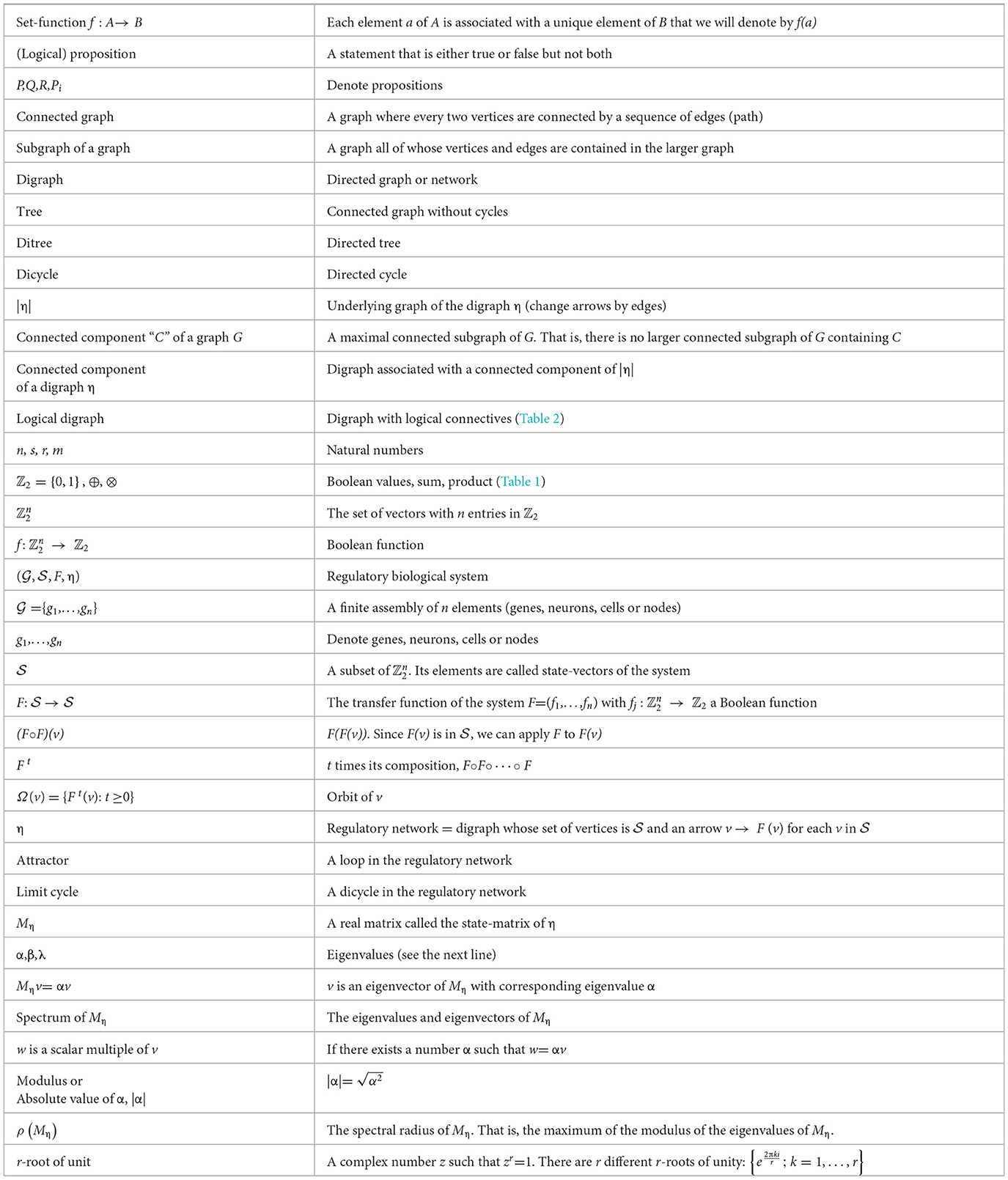
Glossary