Dependence modeling and portfolio optimization with copula-GARCH: a European investment perspective

This study investigates advanced portfolio optimization techniques that integrate copula functions and GARCH models to enhance risk-adjusted performance in the European stock market. Traditional methods, such as mean-variance optimization, often fail to capture non-linear dependencies and heavy-tailed behaviors observed in financial returns. The copula-GARCH framework addresses these limitations by jointly modeling dependence structures and time-varying volatility. Using high-performance computing (HPC) resources, approximately 10,000 portfolios were simulated to evaluate the effectiveness of different copula-GARCH configurations. Several GARCH-type specifications - standard GARCH, GJR-GARCH, and exponential GARCH (eGARCH) - were tested in combination with various copula families. The analysis focused on EURO STOXX 50 constituents, with model estimation based on 2014-2021 data and out-of-sample backtesting conducted across three market regimes: the bearish year 2022, the bullish recovery in 2023, and the neutral conditions of 2024. Performance was benchmarked against traditional mean-variance and historical Conditional Value at Risk (CVaR) optimization methods. The combination of a Student’s t copula [33, 34] with marginal Student’s t distributions and an eGARCH model consistently outperformed alternatives, achieving lower CVaR values while maintaining favorable return profiles. This configuration demonstrated superior ability to capture tail dependence and asymmetric volatility, which contributed to its robustness across diverse market conditions. The findings confirm that copula-GARCH models provide a more realistic and adaptable framework for portfolio construction under changing market dynamics. By capturing both non-linear dependencies and time-varying volatility, this approach improves downside-risk control without compromising returns. These results highlight the practical value of copula-GARCH optimization for risk-averse investors operating in the European equity market.

1 Introduction

Optimizing financial portfolios involves the careful balancing of expected returns against associated risks. Traditional methodologies, such as the mean–variance approach developed by Markowitz (1, 2), have long served as foundational tools in this domain. However, these models often struggle to adequately represent the complex, non-linear relationships and heavy-tailed distributions commonly observed in financial markets (3). In response to these challenges, the integration of copula functions with GARCH (Generalized Autoregressive Conditional Heteroskedasticity) models has emerged as a more flexible and powerful alternative. These methods allow for a more accurate representation of the dynamic dependencies between asset returns and the time-varying nature of market volatility (4), making them particularly useful for risk-sensitive applications. Following Bollerslev (4), we adopt the GARCH framework, and, where relevant, relate it to Engle’s (5) ARCH model. Within the GARCH family, several variants have been proposed to capture different volatility dynamics. In this study, we consider multiple GARCH-type models—specifically, the standard GARCH, GJR-GARCH (6), and Exponential GARCH (7)—to evaluate their performance in modeling asymmetric and time-varying volatility. Among these, the eGARCH model plays a central role in our empirical analysis due to its ability to capture leverage effects and volatility asymmetry, which are prevalent in equity returns.

Asset returns are rarely isolated—co-movements, especially among assets within the same sector or geographical area, are common and can intensify during periods of market stress. Modeling these joint behaviors (8–10) accurately is essential for effective risk assessment and robust portfolio construction. This study employs copula-GARCH models to simulate the behavior of stocks within the EURO STOXX 50 Index, compares their effectiveness to that of conventional optimization strategies, and assesses their implications for portfolio performance and risk management. We use EURO STOXX 50 constituents with daily data from 2014 to 2021 for model estimation and generate out-of-sample evaluations for 2022 (downturn), 2023 (recovery), and 2024 (neutral) regimes. Our motivation is to provide a risk-averse portfolio (11) construction workflow that captures heavy tails and asymmetric dependence neglected by mean–variance methods. We aim to quantify the out-of-sample benefits of copula–GARCH portfolios when the objective is tail-risk minimization (CVaR). Across regimes, portfolios based on a Student’s t copula and eGARCH marginals achieve lower CVaR while maintaining competitive mean returns relative to historical CVaR and mean—variance benchmarks. While the empirical analysis highlights the superior performance of the EGARCH specification, the study systematically compares several GARCH-family models to ensure robustness and consistency in volatility estimation.

Section 2 reviews VaR/ES and volatility modeling; Section 3 details data and estimation; Section 4 reports backtests; Section 5 reports results and discussion; Section 6 concludes.

2 Traditional methods

2.1 Markowitz approach

The Markowitz approach (1), also known as mean–variance analysis, is a fundamental component of Modern Portfolio Theory. It provides a framework for achieving a higher expected portfolio return for a given level of risk, or conversely, minimizing risk for a given expected return. The expected portfolio return is calculated as:

$\begin{array}{ll}E\left(R_p\right)=\sum _{i=1}^n{w}_i\ast E\left(R_i\right),& (1)\end{array}$

where:

• $w_i$ is the weight of the i-th asset in the portfolio,

• $E(R_i$ ) is the expected return of the i-th asset.

This formula allows for the efficient allocation of assets to optimize returns while managing risk.

In the Markowitz model, portfolio risk ${\sigma }_p$ is measured by the standard deviation of returns, where the portfolio variance is calculated as:

$\begin{array}{ll}\mathrm{Var}\left(R_p\right)=\sum _{i=1}^n\sum _{j=1}^n{w}_i\ast w_j\ast cov(R_i,R_j)& (2)\end{array}$

The portfolio risk ${\sigma }_p$ is then:

${\sigma }_p=\sqrt{\mathrm{Var}\left(R_p\right)}$

While Markowitz’s portfolio optimization is a cornerstone of financial theory, its practical application is limited by several assumptions and challenges (12, 13). These include reliance on historical data, sensitivity to input estimates, the assumption of normality, and the neglect of extreme events and multi-period investment horizons. Such limitations underscore the need for more advanced models that better capture the complexities of real-world financial markets (14, 15).

2.2 Value-at-Risk (VaR)

Value-at-Risk (VaR) is one of the most widely used risk measures in financial institutions and regulatory frameworks (16, 17), including its incorporation into the Basel II capital adequacy framework, highlighting its importance in risk management (18). VaR provides a summary measure of the potential loss in value of a financial portfolio (19–21) over a defined time horizon, given a specific confidence level.

To define VaR, three elements are essential: the time horizon (e.g., 1 day or 1 month), the confidence level α (commonly 95% or 99%), and the base currency. Mathematically, the α-level VaR for the loss variable 𝐿 is defined as:

${\mathrm{VaR}}_{\alpha }\left(L\right)=inf\{l\in ℝ:P(L\le l)\ge \alpha \}$

where:

• ${\mathrm{VaR}}_{\alpha }\left(L\right)$ is the Value-at-Risk at confidence level α for the loss variable L. It represents the maximum expected loss over a specified time horizon with probability α,

• L is the random variable representing portfolio losses,

• α is the confidence level (e.g., 95% or 99%).

While VaR is popular, it has limitations—most notably, it does not provide information about losses beyond the VaR threshold (22–24). For this reason, many risk managers prefer Expected Shortfall (ES), also known as Conditional VaR, which captures the average loss in the tail beyond the VaR level. We emphasize Expected Shortfall (ES) (25), also known as CVaR, as a coherent tail-risk measure [see Artzner et al. (26)]. In other words, while VaR only estimates the maximum expected loss at a given confidence level, CVaR goes a step further by quantifying the expected loss assuming that the loss has already exceeded the VaR threshold. This makes it particularly valuable for assessing extreme market scenarios and stress-testing portfolios.

In the context of this study, the CVaR was used as the primary optimization criterion within the copula-GARCH framework (20). This choice reflects a shift from mean–variance thinking to downside risk minimization, recognizing that investors are often more concerned with limiting extreme losses than with general variance.

2.3 GARCH

The GARCH model (4) is a generalization of the ARCH model [the ARCH precursor to GARCH is due to Engle (5)]. A characteristic of the ARCH process is that its conditional standard deviation ${\sigma }_t$ or volatility, is a continuously varying function of the previous values of the square of the process. On the other hand, GARCH is a generalization in the sense that the variance ${\sigma }_t^2$ , or the squared volatility, is allowed to depend on the previous squared fluctuations as well as on the previous squared values of the process itself (1).

The GARCH model (4) is a generalization of the ARCH model, which models time-varying volatility in financial time series. In an ARCH process, the conditional standard deviation ${\sigma }_t$ , or volatility, is a function of previous squared values of the process. GARCH extends this by allowing the conditional variance ${\sigma }_t^2$ to depend not only on past squared fluctuations but also on past values of the variance itself (18).

The GARCH(p, q) process is represented by the following formulas:

$\begin{array}{ll}{X}_t={\sigma }_t{Z}_t,& (3)\end{array}$

$\begin{array}{ll}{\sigma }_t^2={\alpha }_0+\sum _{i=1}^q{\alpha }_i{X}_{t-i}^2+\sum _{j=1}^p{\beta }_j{\sigma }_{t-j}^2,& (4)\end{array}$

where:

• t is time,

• p, q are the orders of the ARCH and GARCH components, respectively,

• ${\alpha }_0$ is a constant,

• ${\sigma }_t^2$ represents the conditional variances,

• ${\alpha }_i$ are the ARCH model parameters,

• ${\beta }_i$ are the GARCH model parameters,

• $X_t$ is the ARCH process,

• $Z_t$ is i.i.d. N(0;1).

σ²ₜ is the conditional variance only if the innovation Z_t follows a standard normal distribution. For heavy-tailed innovations such as the Student’s t, σ² _t represents the conditional scale parameter, and the conditional variance is σ² _t multiplied by the appropriate factor [ν/(ν–2) for ν > 2].

The Equations 3 and 4 model provides crucial insights into the volatility and risk of financial instruments, enabling more accurate risk assessment for portfolios. Additionally, it addresses the limitation of the Markowitz model, which assumes constant volatility, offering a more realistic view of market dynamics.

2.4 Copulas

Copulas (27, 28), first introduced by Sklar [we refer to Sklar’s foundational theorem (29) and the comprehensive monograph by Joe (30) for background on copula modeling], have become increasingly prominent in modern statistics and data analysis (31) due to their flexibility and precision in modeling the joint distribution of multivariate random variables. Their versatility has led to widespread adoption across diverse disciplines such as finance, insurance, econometrics, artificial intelligence, and climatology, while also drawing significant interest from probability theorists.

One of the key advantages of copulas lies in their ability to capture complex dependency structures that traditional methods, such as Pearson correlation, cannot adequately address. While Pearson correlation measures only linear relationships, copulas are capable of modeling non-linear dependencies and are sensitive to the rank-based associations between variables (18). This makes them especially valuable in fields where accurate modeling of interdependence is crucial.

An n-dimensional copula is a function C:[0,1]n → [0,1] that satisfies the following properties (32):

• $\forall u\in [0,1]$ , C(1,…, 1, $u,$ 1,…, 1) = $u,$

• $\forall u\in [0,1]$ , C( $u_1$ ,…, $u_n$ ) = 0, if at least one of $u_i$is equal to zero.

• C is grounded and n-increasing, meaning the C-volume of every box with vertices in ${[0,1]}^n$ is positive.

Panels in Figure 1 were regenerated using a common linear correlation target of ρ ≈ 0.90 across families for comparability and the Gumbel panel was enhanced to highlight upper-tail asymmetry.

Figure 1

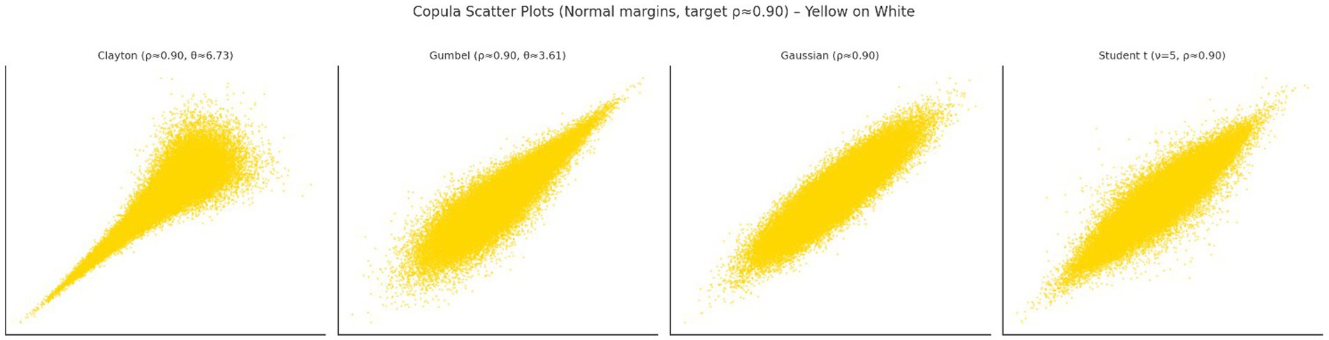
Figure 1. Most popular copula densities in finance.

The copula-GARCH framework offers a more realistic and sophisticated approach to simulating future portfolio performance under various market conditions. By capturing both the intricate dependency structure among assets and the dynamic nature of market volatility, this method significantly enhances stress testing and scenario analysis, thereby supporting more robust asset allocation decisions (33).

Unlike traditional optimization techniques, which often rely on assumptions of linear dependence and constant volatility, the copula-GARCH model accounts for non-linear interactions and time-varying risk. This allows for more accurate identification of diversification opportunities and the construction of portfolios that are less vulnerable to extreme co-movements and large simultaneous losses. As a result, portfolios optimized using this approach tend to achieve superior risk-adjusted returns.

Traditional methods may overlook these nuanced risk characteristics, potentially leading to suboptimal diversification and elevated portfolio risk. In contrast, the copula-GARCH approach offers a more comprehensive and realistic modeling framework by addressing tail dependencies, asymmetries, and volatility clustering. This makes it a potentially more effective tool for asset allocation and risk management in complex and volatile financial environments.

The following sections detail the construction of the copula-GARCH algorithm and present the results of simulation-based portfolio optimization.

3 Algorithm for constructing a portfolio based on copula and GARCH

The investment universe in our study is defined strictly as the EURO STOXX 50. Portfolios are constructed to be long-only, with no leverage or short sales permitted. Each portfolio is positioned fully at inception and then held unchanged throughout the investment horizon. As a result, turnover within the period is exactly zero (12, 13, 34).

Because no rebalancing occurs during the life of the positions, we treat transaction costs and asset holding costs as identical and negligible. This means that all reported results are already net of such costs, without further adjustments.

Finally, when analyzing portfolio risk and performance over time, we ensure consistency in the treatment of returns. Daily portfolio moments are first calculated using standard returns. For longer horizons—such as multi-day or annual periods used in backtests (e.g., for 2022)—these daily returns are converted to log-returns before compounding and Conditional Value-at-Risk (CVaR) evaluation. This method guarantees proper time aggregation and alignment with VaR/ES measurement.

The construction and optimization of a portfolio based on copula and GARCH (4) models can be efficiently accomplished using the following algorithm:

• Stock selection and obtaining logarithmic returns: choose the stocks for the portfolio and compute their logarithmic returns. We compute both standard (simple) returns and log-returns. Equations 1, 2 for portfolio mean and variance are evaluated using standard returns (exact identities), while log-returns are used only for time aggregation across horizons.

• Testing for stationarity and the ARCH effect: verify the stationarity of the return series and test for the presence of the ARCH effect. Stationarity was assessed using Augmented Dickey–Fuller (ADF) (35) and KPSS (36) tests. ARCH effects were tested with Engle’s (5) LM test.

• GARCH model selection: identify the appropriate GARCH model to capture the time-varying volatility in the return series.

• Selection of the marginal distribution: choose the marginal distribution that best fits the individual asset returns.

• Copula selection from transformed standardized GARCH residuals: select a copula function based on the transformed standardized GARCH residuals to model the dependencies between assets. We adopt a two-step inference-for-margins (IFM) procedure: (i) estimate univariate GARCH parameters and marginal distributions; (ii) fit copula parameters to the standardized residuals.

• Simulating returns from the copula function: generate simulated returns using the chosen copula function (21).

• Portfolio optimization using CVAR minimization: optimize the portfolio based on the simulated returns by minimizing CVaR.

The following algorithm was implemented using R Studio and Riga Technical University’s high-performance computing (RTU HPC) infrastructure to extend the portfolio optimization method to 10,000 portfolios. The RTU HPC cluster comprises 34 computing nodes for job execution and one head node responsible for cluster management. All nodes are interconnected via a high-speed InfiniBand network. Each compute node is equipped with two x86_64 architecture processors (CPUs), and some nodes also feature 2 or 4 Nvidia Tesla graphical accelerators (GPUs). The cluster architecture is heterogeneous, combining nodes of varying generations and technical specifications (37). Consequently, 100,000 simulations from the copula function were performed for each stock to achieve maximum likelihood results (see Figure 2).

Figure 2

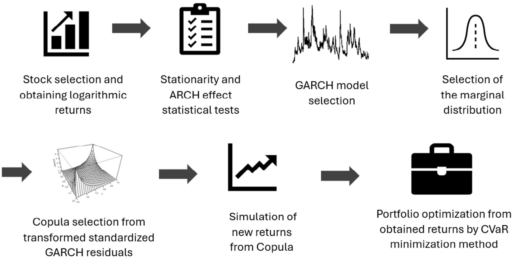
Figure 2. Algorithm for copula-GARCH model-based portfolio optimization.

For each portfolio, 5 stocks were randomly selected from the EURO STOXX 50 index. Each portfolio was optimized using three models: the Markowitz model, the copula-GARCH model with a CVaR minimization approach, and a minimal CVaR model based on historical data. The historical data used for optimization and the estimation of copula and GARCH parameters covered the period from January 1, 2014, to December 31, 2021.

4 Copula and GARCH model selection for EURO STOXX 50 index stocks

To identify the most suitable copula for modelling the dependence structure between asset returns in the EURO STOXX 50 index (38), a comprehensive analysis of all possible pairs of the 50 constituent stocks was conducted. The process involved the following steps (39, 40):

4.1 Data collection

Historical daily closing prices for all 50 stocks in the EURO STOXX 50 index were collected and transformed into log returns to ensure stationarity (41).

4.2 Pairwise analysis

Each of the 1,225 possible pairs of stocks was analyzed to determine the best-fitting copula. The copula families considered included the Gaussian, Clayton, Gumbel, Frank, and Student’s t-copula. In Table 1, you can see the results of the copula selection. Counts correspond to the number of pairs for which each copula family minimizes the information criterion.

Table 1

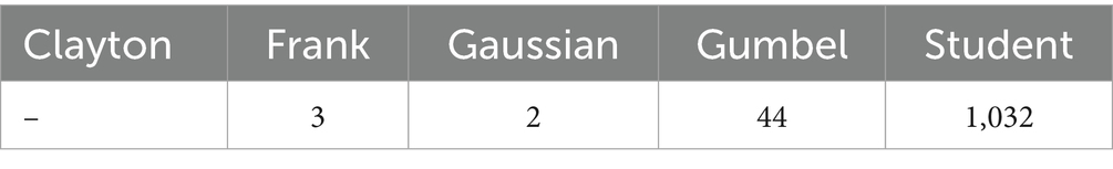
Table 1. Biselectcop() function results for the stocks.

4.3 Goodness-of-fit testing

For each pair, goodness-of-fit tests, such as the Akaike Information Criterion (AIC) and Bayesian Information Criterion (BIC) (42), were used to evaluate the copula models. These tests penalize for model complexity and help in selecting a model that strikes a balance between fit and simplicity.

4.4 Selection criteria

The copula that most frequently emerged as the best fit (43–45) across all pairs was chosen as the most suitable for the entire dataset. This process revealed that the Student’s t-copula was the most appropriate, indicating its effectiveness in capturing the tail dependence and heavy tails characteristic of the joint distribution of stock returns.

To model the conditional volatility of returns, various GARCH models were considered. The process for selecting the most suitable GARCH model involved the following steps:

4.5 Data collection

Historical daily closing prices of the EURO STOXX 50 index were used to compute the index returns.

4.6 Model specification

Various GARCH model variants were considered, including the standard GARCH, GJR GARCH, Integrated GARCH (iGARCH), and Exponential GARCH (eGARCH). The eGARCH model was particularly noted for its ability to capture asymmetries in volatility. For leverage and asymmetry, we consider GJR-GARCH and eGARCH.

4.7 Model evaluation

The suitability of each GARCH model was assessed using information criteria such as the AIC and BIC. These criteria help balance model fit and complexity, ensuring that the selected model is both accurate and parsimonious (please see numerical results in Table 2). Values are averaged across the 50 univariate marginal models (one per stock). Copulas are fitted in a second step to standardized residuals (IFM), i.e., Table 2 does not report joint (marginal and copula) likelihoods.

Table 2

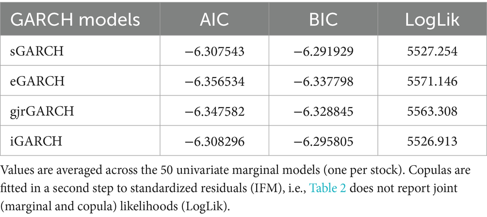
Table 2. GARCH models results.

The eGARCH model emerged as the most suitable for the EURO STOXX 50 index returns due to its superior performance in capturing asymmetric volatility effects. This model effectively accounts for the phenomenon where negative shocks tend to impact volatility more than positive shocks, a common characteristic in financial markets.

5 Results and discussions

The models were tested using data from the year 2022, applying the portfolio weights obtained from the optimization to the selected shares. Profit and loss (PnL) for all portfolios were calculated as of December 29, 2022. The histograms displaying the PnL results are presented in Figure 3.

Figure 3

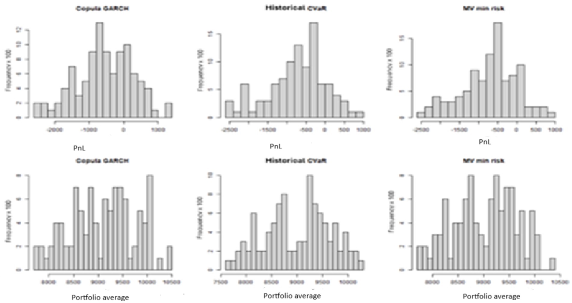
Figure 3. Profit and loss (PnL) histograms as of December 29, 2022.

The copula-GARCH models produced more positive values compared to the other two models. Table 3 provides a summary of the number of instances where each model achieved the highest PnL, along with the minimum, maximum, and average values. Additionally, the table presents the lowest CVaR index and standard deviation for each model.

Table 3

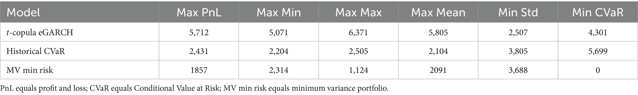
Table 3. The number of positive outcomes for each model.

In 2022, the market experienced a decline due to political events, providing an opportunity to assess the model’s effectiveness in a negative scenario. However, the t-copula eGARCH investment portfolio construction yielded significantly better results. For instance, Figure 4 illustrates the performance of hypothetical portfolios throughout 2022, where the t-copula eGARCH portfolio demonstrates greater resilience to market downturns.

Figure 4

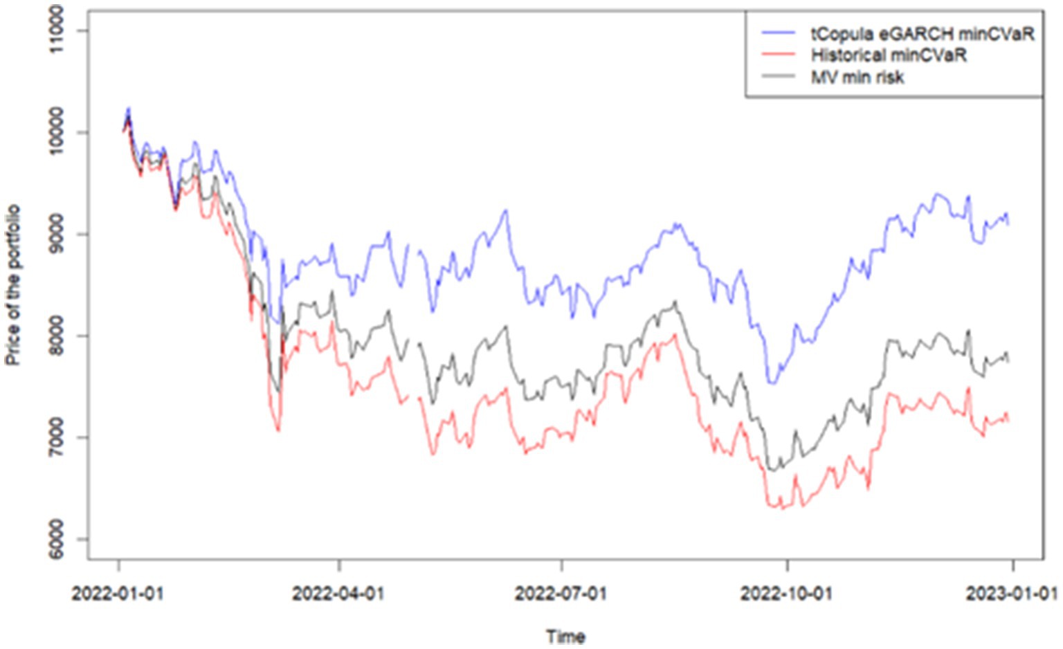
Figure 4. Trajectories of three hypothetical portfolios in 2022.

Table 4 summarizes the portfolio profit and loss (PnL) on 2023-01-01 for various models, including a detailed breakdown of the copula-GARCH model using different copula types.

Table 4

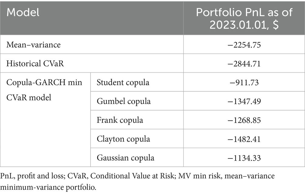
Table 4. Portfolio PnL across different models.

The data indicate that the Student’s t (46, 47) copula yields the most favorable result, with the lowest loss among all models. Figure 5 visualizes the evolution of portfolio values under the copula-GARCH model using different copulas. While the performance trajectories are relatively close, the portfolio constructed with the Student’s t copula consistently outperforms the others.

Figure 5

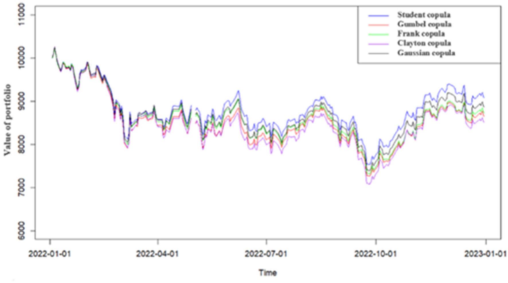
Figure 5. Portfolio value comparison using different copulas in the copula-GARCH model.

Additional backtesting was conducted using data from 2023, a year marked by generally positive market conditions. This provided an opportunity to evaluate the model’s performance under favorable dynamics. As presented in Table 5, the copula-GARCH model outperformed both the historical CVaR and mean–variance models in terms of profit and loss (PnL) in 66% of cases. However, not all performance metrics were in its favor. The minimum CVaR model, based on historical data, more frequently achieved the lowest CVaR values and more often reached the maximum portfolio value compared to the other models.

Table 5

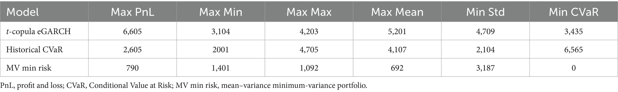
Table 5. The number of positive outcomes for each model.

To further assess the stability and generalizability of the optimization frameworks, a subsequent backtest was performed using 2024 data. In contrast to the pronounced market downturn in 2022 and the strong recovery in 2023, the market environment in 2024 was more neutral, with no clear directional trend and moderate volatility. This created a suitable setting to evaluate model performance under relatively stationary market conditions.

Table 6 summarizes the outcomes of this backtesting, based on 10,000 simulated portfolios generated for each optimization model. The copula-GARCH model again delivered strong results, achieving the highest performance across several key metrics, including Max PnL, Max Mean, Max Min, and lowest CVaR in most instances. The historical CVaR model demonstrated an advantage in achieving the lowest standard deviation, while the mean–variance model showed comparatively weaker performance across all indicators—particularly in terms of downside risk control.

Table 6

Table 6. The number of positive outcomes for each model.

These findings underscore the robustness of the copula-GARCH approach across varying market regimes. Not only does it perform well under stress (as in 2022) and during recovery (as in 2023), but it also maintains its effectiveness in more neutral or transitional periods, such as 2024. This highlights its value as a reliable and adaptive tool for portfolio optimization across diverse market environments.

6 Conclusion

We acknowledge that the present portfolio analysis does not fully incorporate well-documented stylized facts such as heavy tails, volatility clustering, leverage/asymmetry, and long memory (11). Future work will incorporate ARFIMA–FIGARCH marginals (48, 49) with t-innovations, time-varying copulas (50), and formal goodness-of-fit testing (51). Out-of-sample evaluation will include rolling and expanding windows, risk backtesting in the Fissler–Ziegel and Acerbi–Szekely (25) frameworks, turnover constraints and explicit trading costs, and robust baseline comparisons. To mitigate overfitting and data-snooping, future studies will apply White’s Reality Check (2000) and Hansen’s SPA test (2005), and report bootstrap-based uncertainty bands (25, 48–53).

This research investigated the application of copula-GARCH models in portfolio optimization, with a particular focus on enhancing risk management for portfolios of European equities. The study highlights the critical role of proper model calibration—especially in selecting copula families, GARCH specifications, and initial parameters—in achieving accurate and dependable results.

A structured methodological approach was developed, combining an in-depth review of existing literature with extensive empirical testing. Using the R programming language in the RStudio environment, simulations were run on 10,000 portfolios, supported by high-performance computing resources. The model employed a Student’s t-copula to capture tail dependencies between assets and an exponential GARCH (eGARCH) model to account for time-varying and asymmetric volatility.

Across three distinct market conditions—downturn (2022), recovery (2023), and stability (2024)—the copula-GARCH model consistently outperformed traditional optimization methods, including mean–variance and historical CVaR approaches, particularly in minimizing Conditional Value at Risk (CVaR). This consistent performance across diverse regimes affirms the model’s effectiveness in mitigating downside risk without compromising return potential.

By capturing both complex interdependencies and dynamic volatility patterns, the copula-GARCH framework offers a more nuanced and adaptive approach to portfolio construction. The findings of this study support the practical value of CVaR-based optimization using copula-GARCH models, especially in environments marked by non-linear relationships and heightened uncertainty. As such, this approach presents a compelling alternative to conventional optimization techniques for modern portfolio managers seeking improved resilience and performance.

Data availability statement

The raw data supporting the conclusions of this article will be made available by the authors, without undue reservation.

Author contributions

AV: Data curation, Formal analysis, Funding acquisition, Project administration, Resources, Software, Visualization, Writing – original draft, Writing – review & editing. AM: Conceptualization, Data curation, Formal analysis, Funding acquisition, Investigation, Methodology, Project administration, Resources, Software, Supervision, Validation, Visualization, Writing – original draft, Writing – review & editing. JF: Conceptualization, Investigation, Methodology, Supervision, Validation, Writing – original draft, Writing – review & editing.

Funding

The author(s) declare that no financial support was received for the research and/or publication of this article.

Conflict of interest

The authors declare that the research was conducted in the absence of any commercial or financial relationships that could be construed as a potential conflict of interest.

Generative AI statement

The authors declare that no Gen AI was used in the creation of this manuscript.

Any alternative text (alt text) provided alongside figures in this article has been generated by Frontiers with the support of artificial intelligence and reasonable efforts have been made to ensure accuracy, including review by the authors wherever possible. If you identify any issues, please contact us.

Publisher’s note

All claims expressed in this article are solely those of the authors and do not necessarily represent those of their affiliated organizations, or those of the publisher, the editors and the reviewers. Any product that may be evaluated in this article, or claim that may be made by its manufacturer, is not guaranteed or endorsed by the publisher.

Supplementary material

The Supplementary material for this article can be found online at: https://www.frontiersin.org/articles/10.3389/fams.2025.1675120/full#supplementary-material

References

1. Markowitz, HM. Portfolio selection. J Financ. (1952) 7:77–91. doi: 10.1111/j.1540-6261.1952.tb01525.x

Crossref Full Text | Google Scholar

2. Sharpe, WF. The sharpe ratio. J Portf Manag. (1994) 21:49–58. doi: 10.3905/jpm.1994.409501

Crossref Full Text | Google Scholar

3. Natale, FP. Optimization with tail-dependence and tail risk: a copula based approach for strategic asset allocation. Milan: Università degli Studi di Milano-Bicocca, Department of Economics and Management (2006).

Google Scholar

4. Bollerslev, T. Generalized autoregressive conditional heteroscedasticity. J Econom. (1986) 31:307–27. doi: 10.1016/0304-4076(86)90063-1

Crossref Full Text | Google Scholar

5. Engle, R. Autoregressive conditional heteroskedasticity with estimates of the variance of U.K. inflation. Econometrica. (1982) 50:987–1008. doi: 10.2307/1912773

Crossref Full Text | Google Scholar

6. Glosten, LR, Jagannathan, R, and Runkle, DE. On the relation between the expected value and the volatility of the nominal excess return on stocks. J Finance. (1993) 48:1779–801. doi: 10.1111/j.1540-6261.1993.tb05128.x

Crossref Full Text | Google Scholar

7. Nelson, DB. Conditional heteroskedasticity in asset returns: a new approach. Econometrica. (1991) 59:347–70. doi: 10.2307/2938260

Crossref Full Text | Google Scholar

8. Fantazzini, D. Dynamic copula modelling for value at risk. Front Financ Econ. (2008) 5:72–108.

Google Scholar

9. Rosenberg, J, and Schuermann, TA. A general approach to integrated risk management with skewed, fat-tailed risks. J Financ Econ. (2006) 79:569–614. doi: 10.1016/j.jfineco.2005.03.001

Crossref Full Text | Google Scholar

10. Sahamkhadam, M, Stephan, A, and Östermark, R. Copula-based black–Litterman portfolio optimization. Eur J Oper Res. (2022) 297:1055–70. doi: 10.1016/j.ejor.2021.06.015

Crossref Full Text | Google Scholar

11. Cont, R. Empirical properties of asset returns: stylized facts and statistical issues. Quant Finance. (2001) 1:223–36. doi: 10.1080/713665670

Crossref Full Text | Google Scholar

12. Ganti, A., Murry, C., and Veslaquez, V. Efficient frontier: what it is and how investors use it. Investopedia, (2023). Available online at: https://www.investopedia.com/terms/e/efficientfrontier.asp#:~:text=The%20efficient%20frontier%20is%20the,for%20the%20level%20of%20risk (accessed May 19, 2024)

Google Scholar

13. Haugh, M. Mean-variance optimization and the CAPM. IEOR E4706: foundations of financial engineering (2016). Available online at: https://www.columbia.edu/~mh2078/FoundationsFE/MeanVariance-CAPM.pdf (accessed May 19, 2024

Google Scholar

14. Chopra, VK, and Ziemba, WT. The effect of errors in means, variances, and covariances on optimal portfolio choice. J Portf Manag. (1993) 19:6–11. doi: 10.3905/jpm.1993.409440

Crossref Full Text | Google Scholar

15. Taleb, NN. The black swan: the impact of the highly improbable. New York: Random House (2007).

Google Scholar

16. Abad, P, Benitob, S, and López, C. A comprehensive review of value at risk methodologies. Span Rev Financ Econ. (2014) 12:15–32. doi: 10.1016/j.srfe.2013.06.001

Crossref Full Text | Google Scholar

17. Alotaibi, TS, Luciana, DV, and Craven, MJ. The worst case GARCH-copula CVaR approach for portfolio optimisation: evidence from financial markets. J Risk Financ Manag. (2022) 15:1–14. doi: 10.3390/jrfm15100482

Crossref Full Text | Google Scholar

18. McNeil, A, Frey, R, and Embrechts, P. Quantitative risk management: concepts, techniques and tools. Princeton and Oxford: Princeton University Press (2005). 554 p isbn:0-691-12255-5.

Google Scholar

19. Bohdalová, M, and Greguš, M. Portfolio optimization and Sharpe ratio based on copula approach. Res J Econ Bus ICT. (2012) 6:50–56.

Google Scholar

20. Bouye, E., and Salmon, M. Dynamic copula quantile regressions and tail area dynamic dependence in forex markets. Financial Econometrics Research Centre, (2002). Available online at: https://warwick.ac.uk/fac/soc/wbs/subjects/finance/research/wpaperseries/2003/03-121.pdf (accessed 10 May, 2024)

Google Scholar

21. Cech, C. Copula-based top-down approaches in financial risk aggregation. Vienna: University of Applied Sciences (2006).

Google Scholar

22. Chen, X, and Fan, Y. Estimation of copula-based semiparametric time series models. J Econom. (2006) 130:307–35. doi: 10.1016/j.jeconom.2005.02.004

Crossref Full Text | Google Scholar

23. Data Science Genie. Computing the portfolio VAR using copulas. Data Science Genie, (2024). Available online at: https://datasciencegenie.com/computing-the-portfolio-var-using-copulas/ (accessed 15 May, 2024)

Google Scholar

24. Enders, W. Applied econometric time series. Fourth ed. Hoboken, New Jersey: Wiley (2014).

Google Scholar

25. Acerbi, C, and Szekely, B. Backtesting expected shortfall. Risk. (2014) 27:76–81.

Google Scholar

26. Artzner, P, Delbaen, F, Eber, JM, and Heath, D. Thinking coherently. Risk. (1997) 10:68–71.

Google Scholar

27. Frees, EW, and Valdez, EA. Understanding relationships using copulas. N Am Actuar J. (1998) 2:1–25. doi: 10.1080/10920277.1998.10595667

Crossref Full Text | Google Scholar

28. Nelsen, R. An introduction to copulas. Second ed. New York: Springer (2006). 249 p isbn:978-0387-28659-4.

Google Scholar

29. Sklar, A. Fonctions de r’epartition ‘a n dimensionset leurs marges. Publ. Inst. Statis. Univ. (1959). Paris 8, pp.229–231.

Google Scholar

30. Joe, H. Dependence modeling with copulas. Boca Raton, Florida: Chapman & Hall/CRC (2014).

Google Scholar

31. Darsow, W, Nguyen, B, and Olsen, E. Copulas and Markov processes. Ill J Math. (1992) 36:600–42. doi: 10.1215/IJM/1255987328

Crossref Full Text | Google Scholar

32. Malevergne, Y, and Sornette, D. Extreme financial risks: from dependence to risk management. Berlin: Springer (2006). 307 p isbn:978-3-540-27264-9.

Google Scholar

33. Cherubini, U, Luciano, E, and Vecchiato, W. Copula methods in finance. England: John Wiley & Sons (2004).

Google Scholar

34. Francis, J.C., and Kim, D. Modern portfolio theory: foundations, analysis, and new developments. Published by John Wiley & Sons, Inc., Hoboken, New Jersey, (2013).

Google Scholar

35. Dickey, DA, and Fuller, WA. Likelihood ratio statistics for autoregressive time series with a unit root. Econometrica. (1981) 49:1057–72. doi: 10.2307/1912517

Crossref Full Text | Google Scholar

36. Kwiatkowski, D, Phillips, PCB, Schmidt, P, and Shin, Y. Testing the null hypothesis of stationarity against the alternative of a unit root. J Econom. (1992) 54:159–78. doi: 10.1016/0304-4076(92)90104-Y

Crossref Full Text | Google Scholar

37. RTU HPC user manual (2023). Available online at: https://hpc-guide.rtu.lv/index.html (accessed April, 2023)

Google Scholar

38. STOXX. EURO STOXX 50. stoxx.com (2024). Available online at: https://stoxx.com/index/SX5E/# (accessed 15 May, 2024)

Google Scholar

39. Ghalanos, A. Introduction to the rugarch package. RStudio, PBC, (2022). Available online at: https://cran.rproject.org/web/packages/rugarch/vignettes/Introduction_to_the_rugarch_package.pdf (accessed May 15, 2024)

Google Scholar

40. Krzemienowsk, A., and Szymczyk, S. Portfolio optimization with a copula-based extension of conditional value-at-risk. Springerlink.com. Available online at: https://link.springer.com/article/10.1007/s10479-014-1625-3 (accessed May 15, 2024

Google Scholar

41. Statista. Largest stock exchanges in Europe, Middle East, and Africa (EMEA) as of march 2024, by market capitalization of listed companies. Statista, (2024). Available online at: https://www.statista.com/statistics/265251/domestic-market-capitalization-in-europe-the-middle-east-and-africa/ (accessed May 15, 2024)

Google Scholar

42. Hamilton, JD. Time series analysis, vol. 799. New Jersey: Princeton University Press (1994) isbn:978-0691042893.

Google Scholar

43. Tang, A, and Valdez, E. Economic capital and the aggregation of risks using copulas. Sydney: University of New South Wales (UNSW) and University of Connecticut (2006).

Google Scholar

44. Tuan Anh, L, and Thi Thanh Binh, D. Portfolio optimization under mean CVaR simulation with copulas on the Vietnamese stock exchange. Investment management and financial. Innovations. (2021) 18:273–86. doi: 10.21511/imfi.18(2).2021.22

Crossref Full Text | Google Scholar

45. Zhao, Z, Zhou, R, Palomar, DP, and Feng, Y. Portfolio optimization. Piscataway: IEEE Signal Processing Magazine (2019). 2019 p.

Google Scholar

46. Sahamkhadam, M, Stephan, A, and Östermark, R. Portfolio optimization based on GARCH-EVT-copula forecasting models. Int J Forecast. (2018) 34:497–506. doi: 10.1016/j.ijforecast.2018.02.004

Crossref Full Text | Google Scholar

47. Shchankina, A, and Ping, Z. An empirical study on the modelling of an optimal investment portfolio using multivariate model of conditional heteroscedasticity: evidence from the Chinese stock exchanges In: International scientific conference "Far East con" (ISCFEC 2020). China: Atlantis Press SARL (2020)

Google Scholar

48. Granger, CWJ, and Joyeux, R. An introduction to long-memory time series models and fractional differencing. J Time Ser Anal. (1980) 1:15–29. doi: 10.1111/j.1467-9892.1980.tb00297.x

Crossref Full Text | Google Scholar

49. Baillie, RT, Bollerslev, T, and Mikkelsen, HO. Fractionally integrated generalized autoregressive conditional heteroskedasticity. J Econ. (1996) 74:3–30. doi: 10.1016/S0304-4076(95)01749-6

Crossref Full Text | Google Scholar

50. Patton, AJ. Modelling asymmetric exchange rate dependence. J Econ. (2006) 131:231–50. doi: 10.1111/j.1468-2354.2006.00387.x

Crossref Full Text | Google Scholar

51. Genest, C, and Rémillard, B. Validity of the parametric bootstrap for goodness-of-fit testing in semiparametric models. Ann Inst H Poincaré. (2008) 44:1096–127. see also Genest, & B. Rémillard, B. 2009. doi: 10.1214/07-AIHP148

Crossref Full Text | Google Scholar

52. White, H. A reality check for data snooping. Econometrica. (2000) 68:1097–126. doi: 10.1111/1468-0262.00152

Crossref Full Text | Google Scholar

53. Hansen, PR. A test for superior predictive ability. J Bus Econ Stat. (2005) 23:365–80. doi: 10.1198/073500105000000063

Crossref Full Text | Google Scholar