Exploring Class Enumeration in Bayesian Growth Mixture Modeling Based on Conditional Medians

1 Introduction

Growth mixture modeling has been widely used for longitudinal data analyses in social and behavioral research. It is a combination of growth curve modeling (Meredith and Tisak, 1990; Bollen and Curran, 2006) and finite mixture modeling (McLachlan and Peel, 2000). Growth curve modeling is a modeling method for analyzing longitudinal data. It describes the mean growth trajectory and the variability of the individual trajectories around the mean trajectory. The finite mixture modeling is a statistical method to provide accurate statistical inferences when the target population consists of several heterogeneous groups. Mathematically, this is accomplished by modeling an unknown distribution (the target population) using a mixture of known distributions (heterogeneous groups/subpopulations). As a combination of the two methods, growth mixture modeling can handle longitudinal data with several unobserved heterogeneous subpopulations, each of which is characterized by a distinct growth trajectory. Since those groups cannot be directly observed, the groups are called latent groups (or latent classes). A growth curve model can be seen as a growth mixture model with one latent class.

As growth mixture modeling has continued to receive attention, a number of approaches to growth mixture modeling have been developed. Traditional growth mixture modeling is built upon the assumption that latent growth factors and measurement errors are normally distributed. Namely, outcome variables are normally distributed within each class. When data violate this within-class normality assumption, using a traditional growth mixture model may mislead researchers in deciding the number of latent classes or in estimating parameters (Bauer and Curran, 2003; Bauer, 2007; Zhang et al., 2013; Depaoli et al., 2019). In social and behavioral sciences, data often have distributions that are not normal (Micceri, 1989; Cain et al., 2017). Robust methods based on various nonnormal distributions have been developed to address nonnormal data. For instance, Zhang et al. (2013) and Zhang (2016) introduced different types of Bayesian growth curve models by varying the distribution of measurement errors, including t, skewed-normal, and exponential power distributions to address nonnormal data. In Zhang et al. (2013), growth curve models using t distributions outperformed traditional growth curve models in parameter estimation when data had heavy tails or outliers. Lu and Zhang (2014) introduced growth mixture models based on t distributions for those situations in which data have outliers and non-ignorable missingness. Muthén and Asparouhov (2015) used a skewed-t distribution on latent factors to address intrinsically skewed data and showed that the skewed-t growth mixture model prefer a more parsimonious solution than traditional growth mixture modeling for skewed data.

Recently, Tong et al., 2020 and Kim, Tong, Zhou, and Boichuk (under review) proposed a new Bayesian approach for growth modeling using conditional medians. The median is a well-known measure of central tendency that is robust against nonnormality, such as skewed data or data with outliers. Bayesian methods have been widely used in latent variable modeling, including growth mixture modeling (e.g., Lee, 2007; Lu et al., 2011; Zhang et al., 2013; Tong et al., 2020). Bayesian methods allow researchers to incorporate prior information into model estimation and to conduct inferences of complex models through advanced sampling algorithms. Tong et al. (2020) considered conditional medians in Bayesian growth curve modeling and showed that the conditional median approach provided less biased estimates than traditional growth curve modeling when data were not normally distributed. Kim et al. (under review) introduced the conditional median approach in Bayesian growth mixture modeling and showed that the median based approach provided less biased parameter estimates with better convergence rates than traditional growth mixture modeling.

Deciding the number of latent classes is one of the important tasks in growth mixture modeling. There has been a number of studies on selecting the number of latent classes in growth mixture modeling. For example, Bauer and Curran (2003) showed that traditional growth mixture modeling tended to over-extract latent classes when data were non-normally distributed. Nylund et al. (2007), Tofighi and Enders (2008), and Peugh and Fan (2012) evaluated the performance of information-based fit indices such as AIC and BIC and likelihood-based tests in identifying the correct number of latent classes. The performance of the model comparison criteria varied, but they appeared to be influenced by a number of factors, especially the complexity of trajectory shapes and the magnitude of separations of latent classes. Depaoli et al. (2019) and Guerra-Peña et al. (2020) used Student’s t, skewed-t, and skewed-normal distributions on latent factors and explored class enumeration when data satisfied or violated the normality assumption. In Depaoli et al. (2019), the class enumeration was greatly influenced by the degree of latent class separation when the underlying population consisted of heterogenous subgroups. In Guerra-Peña et al. (2020), the growth mixture modeling with skewed-t successfully maintained the Type 1 error rate when the underlying population was homogeneous but had a skewed or kurtic distribution.

The median-based growth mixture modeling approach in longitudinal data analysis is relatively new, and its performance has not been systematically investigated. In particular, little is known about the performance of the median-based growth mixture modeling in deciding the number of latent classes. To fill this gap, in this study, we explore this topic within a Bayesian framework. Two simulation studies were conducted to answer the following research questions: 1) how well do Bayesian model comparison criteria used in a growth mixture model analysis correctly identify the number of latent classes when the population is heterogeneous and the normality assumption holds? and 2) how well does the median-based growth mixture modeling perform in identifying the correct number of latent classes when the population is heterogeneous and contains outliers? We examined the class enumeration performance of the median-based growth mixture modeling and compared it to that for the traditional growth mixture modeling and growth mixture modeling based on t-distributed measurement errors, which is also known to be robust to nonnormal data in growth mixture modeling (Zhang et al., 2013; Lu and Zhang, 2014). For model selection, we used three Bayesian model comparison criteria: deviance information criterion (DIC; Spiegelhalter et al., 2002), Watanabe-Akaike information criterion (WAIC; Watanabe, 2010), and leave-one-out cross-validation (LOO-CV; Gelman et al., 2013; Vehtari et al., 2017). DIC is a widely used model comparison criterion in Bayesian analyses. WAIC and LOO-CV are relatively new criteria but have been increasingly used in Bayesian model comparison.

The rest of this paper is organized as follows. We first briefly describe three different growth mixture modeling approaches considered in this study: traditional growth mixture modeling, growth mixture modeling based on t distributions, and growth mixture modeling based on conditional medians. In the subsequent section, we present results of the two simulation studies. The first simulation study presents the performance of DIC, WAIC, and LOO-CV used in the three types of growth mixture models when data are normally distributed within each class. The first simulation study was particularly designed to investigate whether the DIC, WAIC, and LOO-CV are reliable criteria before we consider nonnormal data. Then, the second simulation study evaluates the performance of the three types of growth mixture models when data contain outliers. We mainly examined the impact of outliers on class enumeration and parameter estimates. We end this article with a discussion and concluding remarks.

2 Growth Mixture Models (GMMs)

2.1 Traditional Approach (Traditional GMM)

Growth mixture models (GMMs) are designed to detect subpopulations that have distinct patterns of growth trajectory. Suppose that a population consisted of G subgroups (or latent classes) that have distinct patterns of change. Let ${\mathit{y}}_i={\left(y_{i1},\dots ,y_{iT}\right)}^{\text{'}}$ is a vector of T repeated observations for individual i ($i\in \left\{1,\dots ,N\right\}$) that belongs to class g. Then, a general form of growth mixture models can be specified as

${\mathit{y}}_i|(z_i=g)=\mathbf{\Lambda }{\mathit{b}}_{ig}+{\mathrm{ϵ}}_i,$

where $\mathbf{\Lambda }$ is a $T\times q$ matrix of factor loadings that determines the shape of the growth trajectories, ${\mathit{b}}_{ig}$ is a $q\times 1$ vector of latent factors for class g, ${\mathrm{ϵ}}_i={\left({\mathit{ϵ}}_{i1},\dots ,{\mathit{ϵ}}_{iT}\right)}^{\text{'}}$ is a $T\times 1$ vector of measurement errors, and $z_i$ represents a class indicator with $P(z_i=g)={\pi }_g$. The latent factors are usually assumed as ${\mathit{b}}_{ig}\sim N_q\left({\mathit{\beta }}_g,{\mathbf{\Psi }}_g\right)$, where ${\mathit{\beta }}_g$ is a mean of ${\mathit{b}}_{ig}$ and ${\mathbf{\Psi }}_g$ is a variance-covariance matrix of ${\mathit{b}}_{ig}$. The measurement errors are typically assumed to follow a normal distribution, ${\mathrm{ϵ}}_i\sim N_T\left(0,{\mathbf{\Sigma }}_g\right)$. This assumption leads the conditional mean of ${\mathit{y}}_i$ given ${\mathit{b}}_{ig}$ to be $E\left({\mathit{y}}_i|{\mathit{b}}_{ig}\right)=\mathbf{\Lambda }{\mathit{b}}_{ig}$. It is common to further assume that the measurement errors have equal variances across time and are independent of each other. That is, ${\mathbf{\Sigma }}_g={\sigma }_g^2\mathit{I}$, where ${\sigma }_g^2$ is a scale parameter for class g. We assumed this measurement error structure for the rest of this study.

2.2 t-Based Approach (t-Based GMM)

The traditional GMM is built based upon the assumption that data within each class is normally distributed. However, when data do not satisfy this assumption, the traditional approach may lead to inappropriate conclusions such as biased parameter estimates or over-extraction of latent classes. As a robust approach to the traditional growth mixture modeling, t distributions have been used in growth mixture modeling, as they downweight extreme values in the model estimation process (Zhang et al., 2013; Lu and Zhang, 2014). In this growth mixture modeling approach, a multivariate t distribution can be assumed on the latent factors or measurement errors (Tong and Zhang, 2012; Lu and Zhang, 2014). In this study, for the t-based growth mixture modeling approach, we assumed that the measurement errors follow a multivariate t distribution,

${\mathrm{ϵ}}_i\sim M{T}_T\left(0,{\mathbf{\Sigma }}_g,{\nu }_g\right),$

where ${\nu }_g$ is the degrees of freedom, 0 is the mean of ${\mathrm{ϵ}}_i$, and ${\mathbf{\Sigma }}_g$ is a $T\times T$ scale matrix. Then, the distribution of ${\mathit{y}}_i$ conditioning on ${\mathit{b}}_{ig}$ can be written as ${\mathit{y}}_i|{\mathit{b}}_{ig}\sim M{T}_T\left(\mathbf{\Lambda }{\mathit{b}}_{ig},{\mathbf{\Sigma }}_g,{\nu }_g\right)$.

2.3 Median-Based Approach (Median-Based GMM)

In growth mixture modeling based on conditional medians, it considers medians instead of means so that the growth mixture model can be more tolerant of non-normally distributed data (Kim et al., under review). A general form of median-based growth mixture models is specified as follows:

$y_{it}|(z_i=g)={\mathbf{\Lambda }}_t{\mathit{b}}_{ig\left(0.5\right)}+{\mathit{ϵ}}_{it},Q_{0.5}\left(y_{it}\right|{\mathit{b}}_{ig\left(0.5\right)})={\mathbf{\Lambda }}_t{\mathit{b}}_{ig\left(0.5\right)},$

where $Q_{0.5}(\cdot )$ represents the median, ${\mathbf{\Lambda }}_t$ is the t-th row of $\mathbf{\Lambda }$, ${\mathit{b}}_{ig\left(0.5\right)}$ is a vector of latent factors for the median-based model. This median based approach is established based on a Laplace distribution. That is, ${\mathit{ϵ}}_{it}$ follows a Laplace distribution, as the sample median can be viewed as the maximum likelihood estimate of a Laplace distribution (Yu and Moyeed, 2001; Geraci and Bottai, 2007; Yi and He, 2009). A Laplace distribution has two parameters: a location parameter (μ) and a scale parameter (δ). In this model, ${\mathit{ϵ}}_{it}$ follows a Laplace distribution with a location value of 0 and an unknown scale ${\delta }_g$ (${\mathit{ϵ}}_{it}\sim LD\left(0,{\delta }_g\right)$). Then, the distribution of $y_{it}$ conditioning on ${\mathit{b}}_{ig\left(0.5\right)}$ can be written as $y_{it}|{\mathit{b}}_{ig\left(0.5\right)}\sim LD\left({\mathbf{\Lambda }}_t{\mathit{b}}_{ig\left(0.5\right)},{\delta }_g\right)$.

3 Bayesian Estimation

To estimate parameters of the three types of growth mixture models, we used Bayesian methods. In this study, we used JAGS to estimate model parameters. JAGS is a program for Bayesian analysis using Markov chain Monte Carlo (MCMC) algorithms. We used the rjags package (Plummer, 2017) to run JAGS in R (R Core Team, 2019).

For the traditional GMM, the joint distribution of ${\mathit{y}}_i,{\mathit{b}}_i,$ and $z_i$ is

$f\left({\mathit{y}}_i,{\mathit{b}}_i,z_i|{\mathit{\beta }}_{1:G},{\mathbf{\Psi }}_{1:G},{\sigma }_{1:G}^2,\mathit{\pi }\right)=f\left({\mathit{y}}_i|{\mathit{b}}_i,z_i,{\sigma }_{1:G}^2\right)f\left({\mathit{b}}_i|{\mathit{\beta }}_{1:G},{\mathbf{\Psi }}_{1:G},z_i\right)p\left(z_i|\mathit{\pi }\right).$

The complete likelihood (Celeux et al., 2006) for the traditional GMM is

$L_c={\displaystyle \prod }_{i=1}^{N}f\left({\mathit{y}}_i,{\mathit{b}}_i,z_i|{\mathit{\beta }}_{1:G},{\mathbf{\Psi }}_{1:G},{\sigma }_{1:G}^2,\mathit{\pi }\right).$

The following priors were used to estimate the traditional growth mixture model: ${\mathit{\beta }}_g\sim N_q\left({\mathit{\beta }}_0,{\mathbf{\Sigma }}_0\right)$, ${\mathbf{\Psi }}_g\sim InvWishart\left({\nu }_0,S_0\right)$, ${\sigma }_g^2\sim InvGamma\left(c_0,d_0\right)$ for $g=1,\dots ,G$, and $\mathit{\pi }\sim Dirichlet\left(\mathit{\zeta }\right)$.

For the t-based GMM, we used a normal distribution and gamma distribution to construct a multivariate t distribution to simplify the posterior distribution (Kotz and Nadarajah, 2004; Zhang et al., 2013). If ${\mathit{y}}_i|{\mathit{b}}_{ig}\sim M{T}_T\left(\mathbf{\Lambda }{\mathit{b}}_{ig},{\sigma }_g^2\mathit{I},{\nu }_g\right)$, then it can be represented as ${\mathit{y}}_i|{\mathit{b}}_{ig},{\omega }_i\sim M{N}_T\left(\mathbf{\Lambda }{\mathit{b}}_{\mathit{ig}},\frac{{\sigma }_g^2}{{\omega }_i}\mathit{I}\right)$, where ${\omega }_i\sim Gamma\left({\nu }_g/2,{\nu }_g/2\right)$. In this approach, the joint distribution of ${\mathit{y}}_i,{\mathit{b}}_i,$$z_i$, and ${\omega }_i$ is

$f\left({\mathit{y}}_i,{\mathit{b}}_i,z_i,{\omega }_i|{\mathit{\beta }}_{1:G},{\mathbf{\Psi }}_{1:G},{\sigma }_{1:G}^2,{\nu }_{1:G},\mathit{\pi }\right)=f\left({\mathit{y}}_i|{\mathit{b}}_i,z_i,{\omega }_i,{\sigma }_{1:G}^2\right)f\left({\mathit{b}}_i|{\mathit{\beta }}_{1:G},{\mathbf{\Psi }}_{1:G},z_i\right)f\left({\omega }_i|{\nu }_{1:G}\right)p\left(z_i|\mathit{\pi }\right).$

The complete likelihood for the t-based GMM is

$L_c={\displaystyle \prod }_{i=1}^{N}f\left({\mathit{y}}_i,{\mathit{b}}_i,z_i,{\omega }_i|{\mathit{\beta }}_{1:G},{\mathbf{\Psi }}_{1:G},{\sigma }_{1:G}^2,{\nu }_{1:G},\mathit{\pi }\right).$

The following prior was additionally used to estimate the t-based GMM: ${\nu }_g\sim Exp\left(k_0\right)$, where $Exp$ denotes the exponential distribution.

For the median-based GMM, the joint distribution of ${\mathit{y}}_i$, ${\mathit{b}}_i$, and $z_i$ is

$f\left({\mathit{y}}_i,{\mathit{b}}_i,z_i|{\mathit{\beta }}_{1:G},{\mathbf{\Psi }}_{1:G},{\delta }_{1:G},\mathit{\pi }\right)=f\left({\mathit{y}}_i|{\mathit{b}}_i,z_i,{\delta }_{1:G}\right)f\left({\mathit{b}}_i|{\mathit{\beta }}_{1:G},{\mathbf{\Psi }}_{1:G},z_i\right)p\left(z_i|\mathit{\pi }\right).$

The complete likelihood for the median-based GMM is

$L_c={\displaystyle \prod }_{i=1}^{N}f\left({\mathit{y}}_i,{\mathit{b}}_i,z_i|{\mathit{\beta }}_{1:G},{\mathbf{\Psi }}_{1:G},{\delta }_{1:G},\mathit{\pi }\right).$

The following prior was additionally used to estimate the median-based GMM: ${\delta }_g\sim InvGamma\left(c_0,d_0\right)$.

4 Model Selection

We used DIC (Spiegelhalter et al., 2002), WAIC (Watanabe, 2010), and LOO-CV (Gelman et al., 2013; Vehtari et al., 2017) to select the number of latent classes for the traditional, t-based, and median-based GMMs. In the following, we briefly introduce the three model comparison criteria.

DIC has been widely used in Bayesian model selection. It was first introduced by Spiegelhalter et al. (2002). DIC is defined based on the concept of deviance and the effective number of model parameters. The deviance is defined as

$D\left(\mathbf{\Theta }\right)=-2l\left(\mathbf{\Theta }\right)+2log\left(h\left(x\right)\right),$

where $\mathbf{\Theta }$ is a set of model parameters, $l\left(\mathbf{\Theta }\right)$ is a log-likelihood, $l\left(\mathbf{\Theta }\right)=log\left(f\left(y|\mathbf{\Theta }\right)\right)$, and $h\left(x\right)$ is a constant that is canceled out when comparing models. The effective number of parameters ($p_D$) is defined as

$p_D=\overline{D\left(\mathbf{\Theta }\right)}-D\left(\overline{\Theta }\right),$

where $D\left(\overline{\Theta }\right)$ is the deviance calculated at the posterior mean of $\mathbf{\Theta }$, and $\overline{D\left(\mathbf{\Theta }\right)}$ is the posterior mean of $D\left(\mathbf{\Theta }\right)$. Combining these two, DIC becomes

$DIC=D\left(\overline{\Theta }\right)+2p_D.$

Models with smaller DICs are preferred.

WAIC is a relatively recently developed Bayesian model comparison criterion. We used the following definition of WAIC (Gelman et al., 2013).

$WAIC=-2\times {\displaystyle \sum }_{i=1}^N\text{log}\left(\frac{1}{S}{\displaystyle \sum }_{s=1}^{S}f\left(y_i|{\mathbf{\Theta }}^{\left(s\right)}\right)\right)+2\times {\displaystyle \sum }_{i=1}^{N}Va{r}_{s=1}^{S}l\left({\mathbf{\Theta }}^{\left(s\right)}\right),$

where S is the number of MCMC iterations, and ${\mathbf{\Theta }}^{\left(s\right)}$ is a draw from the posterior distribution at the sth iteration. Models with smaller WAICs are preferred.

LOO-CV evaluates the model fit based on an estimate of the log predictive density of the hold-out data. Each data point is taken out at a time to cross-validate the model that is fitted based on the remaining data. WAIC has been shown to be asymptotically equal to LOO-CV (Watanabe, 2010). Vehtari et al. (2017) introduced a method to approximate LOO-CV using Pareto-smoothed importance sampling, and this is implemented in the loo package (Vehtari et al., 2019) in R.

We computed the three model comparison criteria based on marginal likelihoods as recommended in Merkle et al. (2019). The traditional GMM has a closed form of the marginal likelihood:

$\begin{array}{c}{L}_N\left(\mathbf{\Theta }\right)=\stackrel{N}{{\displaystyle \prod }_{i=1}}f\left({\mathit{y}}_i|{\mathit{\beta }}_{1:G},{\mathbf{\Psi }}_{1:G},{\sigma }_{1:G}^2,\mathit{\pi }\right)\\ =\stackrel{N}{{\displaystyle \prod }_{i=1}}{\displaystyle \sum }_{z_i}f\left({\mathit{y}}_i,z_i|{\mathit{\beta }}_{1:G},{\mathbf{\Psi }}_{1:G},{\sigma }_{1:G}^2,\mathit{\pi }\right)\\ =\stackrel{N}{{\displaystyle \prod }_{i=1}}\stackrel{G}{{\displaystyle \sum }_{g=1}}{\pi }_{g}f\left({\mathit{y}}_i|{\mathit{\beta }}_g,{\mathbf{\Psi }}_g,{\sigma }_g^2\right),\end{array}$

where $f\left({\mathit{y}}_i|{\mathit{\beta }}_g,{\mathbf{\Psi }}_g,{\sigma }_g^2\right)=\text{Φ}\left({\mathit{y}}_i|\mathbf{\Lambda }{\mathit{\beta }}_g,\mathbf{\Lambda }{\mathbf{\Psi }}_g{\mathbf{\Lambda }}^{\text{'}}+{\sigma }_g^2\mathit{I}\right)$, in which $\text{Φ}(\cdot |\mathit{\mu },\mathbf{\Sigma })$ represents a multivariate normal density function with mean $\mathit{\mu }$ and variance-covariance matrix $\mathbf{\Sigma }$.

The marginal likelihoods of the t-based and median-based GMMs, however, do not have closed forms. For the t-based GMM, the marginal likelihood is

$\begin{array}{c}{L}_T\left(\mathbf{\Theta }\right)=\stackrel{N}{{\displaystyle \prod }_{i=1}}f\left({\mathit{y}}_i|{\mathit{\beta }}_{1:G},{\mathbf{\Psi }}_{1:G},{\sigma }_{1:G}^2,{\nu }_{1:G},\mathit{\pi }\right)\\ =\stackrel{N}{{\displaystyle \prod }_{i=1}}{\displaystyle \sum }_{z_i}{{\displaystyle \int }}^{\text{}}f\left({\mathit{y}}_i,{\omega }_i,z_i|{\mathit{\beta }}_{1:G},{\mathbf{\Psi }}_{1:G},{\sigma }_{1:G}^2,{\nu }_{1:G},\mathit{\pi }\right)d{\omega }_i\\ =\stackrel{N}{{\displaystyle \prod }_{i=1}}\stackrel{G}{{\displaystyle \sum }_{g=1}}{\pi }_g{{\displaystyle \int }}^{\text{}}f\left({\mathit{y}}_i|{\mathit{\beta }}_g,{\mathbf{\Psi }}_g,{\omega }_i,{\sigma }_g\right)f\left({\omega }_i|{\nu }_g\right)d{\omega }_i.\end{array}$

For the median-based GMM, the marginal likelihood is

$\begin{array}{c}{L}_M\left(\mathbf{\Theta }\right)=\stackrel{N}{{\displaystyle \prod }_{i=1}}f\left({\mathit{y}}_i|{\mathit{\beta }}_{1:G},{\mathbf{\Psi }}_{1:G},{\delta }_{1:G},\mathit{\pi }\right)\\ =\stackrel{N}{{\displaystyle \prod }_{i=1}}{\displaystyle \sum }_{z_i}{{\displaystyle \int }}^{\text{}}f\left({\mathit{y}}_i,{\mathit{b}}_i,z_i|{\mathit{\beta }}_{1:G},{\mathbf{\Psi }}_{1:G},{\delta }_{1:G},\mathit{\pi }\right)d{\mathit{b}}_i\\ =\stackrel{N}{{\displaystyle \prod }_{i=1}}\stackrel{G}{{\displaystyle \sum }_{g=1}}{\pi }_g{{\displaystyle \int }}^{\text{}}f\left({\mathit{y}}_i|{\mathit{b}}_i,{\delta }_g\right)f\left({\mathit{b}}_i|{\mathit{\beta }}_g,{\mathbf{\Psi }}_g\right)d{\mathit{b}}_i.\end{array}$

Since ${{\displaystyle \int }}^{\text{}}f\left({\mathit{y}}_i|{\mathit{\beta }}_g,{\mathbf{\Psi }}_g,{\omega }_i,{\sigma }_g\right)f\left({\omega }_i|{\nu }_g\right)d{\omega }_i$ and ${{\displaystyle \int }}^{\text{}}f\left({\mathit{y}}_i|{\mathit{b}}_i,{\delta }_g\right)f\left({\mathit{b}}_i|{\mathit{\beta }}_g,{\mathbf{\Psi }}_g\right)d{\mathit{b}}_i$ do not have closed forms, we used the integrate function and hcubature function in the cubature package in R (Narasimhan et al., 2020) to numerically evaluate the one-dimensional and multidimensional integrals, respectively. Both functions provide an estimate with a relative error of the integration. In this study, the error was required to be less than 0.0001.

5 Simulation Studies

In this section, we evaluated the performance of the three Bayesian model comparison criteria and the performance of the three types of growth mixture models in identifying the correct number of latent classes. Two simulation studies are presented. In the first study, we examined the performance of DIC, WAIC, and LOO-CV used in the traditional GMM, median-based GMM, and t-based GMM when data followed the within-class normality assumption. In the second study, we explored the impact of outliers on identifying the number of latent classes for each of the growth mixture models to evaluate the performance of the median-based GMM and compare it to the performance of the traditional GMM and t-based GMM. For both simulation studies, we also obtained parameter estimation bias to examine how well each of the growth mixture models recover parameters when the number of latent classes was correctly specified.

5.1 Study 1: Examining the Performance of Bayesian Model Comparison Criteria

5.1.1 Simulation Design

In the first simulation study, we report the accuracy of selecting a correct model using DIC, WAIC, and LOO-CV. Data were generated using a traditional two-class linear growth mixture model with four equally spaced time points. Mean trajectories from the two classes were set to have different intercepts and slopes. Parameter values for data generating model were set to be similar to those used for the simulation study in Nylund et al. (2007). In Nylund et al., the bootstrap likelihood ratio test (BLRT; McLachlan, 1987) and Bayesian information criterion (BIC; Schwarz, 1978) identified the correct number of latent classes with high accuracy rates. The first class was characterized as having increasing scores over time (${\beta }_1={\left(\mathrm{2,0.5}\right)}^{\text{'}}$), and the second class was characterized as a flat line (${\beta }_2={\left(\mathrm{1,0}\right)}^{\text{'}}$). The variance-covariance matrix and residual variance were set to be $\mathbf{\Sigma }=\left(\begin{array}{cc}0.25& 0\\ 0& 0.04\end{array}\right)$ and ${\sigma }^2=0.2$, and they were assumed to be the same across the two latent classes. The two groups of growth trajectories in this setting have a Mahalanobis distance¹ ($MD$) value of 3.2, which indicates that the two groups are well-separated (Lubke and Neale, 2006). We also considered a condition with a lower degree of class separation by manipulating the intercept of the first class, ${\beta }_1={\left(1.5,0.5\right)}^{\text{'}}$, which had $MD=2.7$. Mixing proportions were set to be unbalanced: 75% from the first class and 25% from the second class. Two different sample sizes were considered (N = 300, 500). Figure 1 depicts some examples of simulated individual growth trajectories when $MD=2.7$ (left panel) and $MD=3.2$ (right panel). For each of the conditions, we replicated 200 datasets.

FIGURE 1

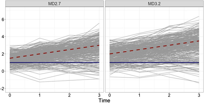
FIGURE 1. Examples of simulated 300 individual growth trajectories from two groups that are relatively close to each other ($MD=2.7$, left panel) and two groups that are relatively far away from each other ($MD=3.2$, right panel). For each panel, the red dashed line indicates the growth trajectory for the first class and the blue solid line indicates the growth trajectory for the second class.

5.1.2 Estimation

In order to evaluate the three model comparison criteria in identifying the correct number of latent classes, we fitted a series of growth mixture models that differed in the number of latent classes (one, two, and three classes). For the purpose of comparison, three different growth mixture modeling approaches were considered: traditional GMM, median-based GMM, and t-based GMM. The following priors were used for model inferences: $p\left({\mathit{\beta }}_g\right)=MN\left(0,{10}^3\times \mathit{I}\right)$ for $g\in \left\{\mathrm{1,2,3}\right\}$, $p\left(\mathbf{\Psi }\right)=InvWishart\left(2,{\mathit{I}}_2\right)$, $p\left({\sigma }^2\right)=InvGamma\left(.01,.01\right)$, $p\left(\nu \right)=Exp\left(0.1\right)$, and $p\left(\mathit{\pi }\right)\sim Dirichlet\left(10{\mathit{j}}_G\right)$, where G is the number of latent classes, and ${\mathit{j}}_G$ is a $G\times 1$ vector that has one for all components for $G>1$. These priors were set to have little information about the parameters. The total number of iterations was $\mathrm{10,000}$, and the first half of the iterations were discarded for burn-in. The convergence of Markov chains was evaluated by the Geweke’s convergence test (Geweke, 1991). Our simulation results were summarized based on replications in which all the three models (one-, two-, and three-class models) were converged for each modeling method. The convergence of chains can be influenced by starting values. The $\mathrm{10,000}$ iterations appeared to be enough, but we allowed each model to be fitted with 10 different starting values at most to obtain converged results. Additionally, the parameter space for the mean intercept was constrained in order to avoid label switching problems.

5.1.3 Results

The proportion of datasets that converged for each condition is shown in Table 1. All models showed adequate convergence rates in all conditions with rates ranging from 0.97 to 1.00 for the traditional GMM, 0.93 to 1.00 for the median-based GMM, and 0.95 to 1.00 for the t-based GMM.

TABLE 1

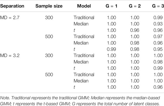
TABLE 1. Proportion of converged datasets.

For each condition, model comparison was examined using DIC, WAIC, and LOO-CV for the traditional, median-based, and t-based GMMs. We compared values across one-, two-, and three-class models and selected the most preferred model using each of the criteria. For DIC, a model with a smaller DIC was preferred over the other competing parsimonious models if the difference in their DIC values were larger than 10 (Lunn et al., 2012). For WAIC and LOO-CV, the loo package provides a function for comparing competing models. When comparing two models, the function estimates the difference in their expected predictive accuracy and the standard error of the difference, which provides the degree of uncertainty in the difference. We selected models based on the differences that are significantly different from 0.

The model selection results are shown in Table 2. In general, the performance of DIC, WAIC, and LOO-CV were influenced by the degree of class separation and sample size. All three criteria had quite high proportions of correct model selection when the degree of class separation was high (i.e., $MD=3.2$) or sample size was large (i.e., N = 500). Under the conditions with $MD=3.2$, the three criteria performed well in correctly discovering the two-class model across the three types of growth mixture models. The three criteria chose the correct model over 98% of the time for the traditional GMM, over 94% of the time for the median-based GMM, and over 97% of the time for the t-based GMM. Under the conditions with $MD=2.7$, DIC had higher selection accuracy than WAIC and LOO-CV across the three different growth mixture models. For example, when sample size was 300, DIC preferred the data generating two-class model about 40% of the time, and WAIC and LOO-CV preferred the two-class model less than 30% of the time.

TABLE 2

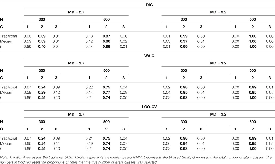
TABLE 2. Proportion for selecting 1-class, 2-class, and 3-class models using DIC, WAIC, and LOO-CV.

Figure 2 presents the magnitude of absolute bias in the intercept and slope parameter estimates for each of the growth mixture models when the number of latent classes was the same as the data generating model. We calculated absolute bias for each model parameter, and Figure 2 shows the absolute bias that averaged over fixed parameters to compare the parameter estimates for the three types of growth mixture models. When data followed the within-class normality assumption, the three types of growth mixture models had similar bias values. All three models tended to have smaller bias when there was a higher degree of latent class separation (i.e., $MD=3.2$) or a larger sample size (i.e., N = 500). Note that the performance of variance-covariance components also had similar patterns of absolute bias.

FIGURE 2

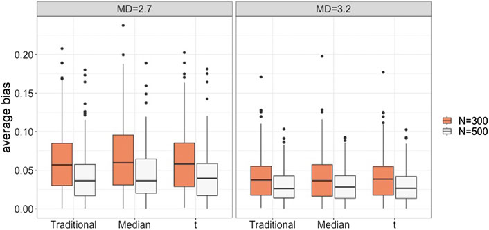
FIGURE 2. Average absolute bias for the traditional, the median-based, and the t-based GMM in conditions with varied degrees of latent class separation and sample sizes.

5.2 Study 2: Examining the Impact of Outliers on Class Enumeration

5.2.1 Simulation Design

In the first simulation study, we presented the performance of the three Bayesian model comparison criteria when data were generated from a normal distribution within each class. The results showed that the performance of the criteria depended on the degree of latent class separation and sample size. When latent classes were well separated (i.e., conditions with $MD=3.2$), the three criteria selected the true model with high proportions. In Study 2, we designed our simulation study based on the conditions with $MD=3.2$, so that we can clearly examine how outliers influence class enumeration. In this simulation study, we manipulated sample size (N = 300, 500) and percentage of outliers (5, 10, and 15%). The other aspects of the simulation design (population model, parameter values, and mixing proportions) were the same as those in Study 1. Subjects in the first latent class were set to have outliers for simplicity. In order to generate data with outliers, $r\text{\%}$ ($r\in \left\{\mathrm{5,10,15}\right\}$) of subjects in the first latent class were randomly selected to have outliers at arbitrarily selected measurement occasions. The outliers were set to be higher than the majority of observations by generating measurement errors from $N\left(C\sigma ,{\sigma }^2\right)$, where C was randomly selected from $\left\{\mathrm{3,5,10}\right\}$ with probabilities 0.4, 0.4, and 0.2, respectively. We considered 200 replications for each condition.

For each dataset, we fitted a series of growth mixture models that differed in the number of latent classes (one-, two-, and three-latent classes) using the traditional GMM, median-based GMM, and t-based GMM. The prior specification and model estimation for this study were in the same way as those described in Study 1.

5.2.2 Results

The proportion of datasets that converged for each condition is shown in Table 3. The three types of growth mixture models showed adequate convergence rates when the number of latent classes was 1 or 2. For the three-class growth mixture model, the traditional GMM had lower convergence rates when the percentage of outliers increased. The t-based and median-based GMM had convergence rates over 0.97 across all conditions.

TABLE 3

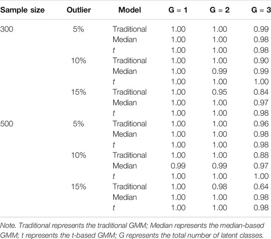
TABLE 3. Proportion of converged datasets.

Tables 4, 5 show the impact of outliers on class enumeration for the three types of growth mixture models. The proportions of selecting 1-class, 2-class, and 3-class models using DIC, WAIC, and LOO-CV are reported for the traditional GMM, median-based GMM, and t-based GMM across all conditions. In the traditional GMM, the model selection accuracy was the lowest among the three models. Different from the other growth mixture models, WAIC and LOO-CV performed better than DIC in model selection (except for the condition with N = 300 and 5% of outliers). When the percentage of outliers increased, the accuracy dropped noticeably. When the percentage of outliers was 15, WAIC and LOO-CV preferred the two-class model only in about 40% of the time for the traditional GMM. When N = 500, in particular, the traditional GMM tended to select the more complicated 3-class model, treating outliers as from an additional class. In the median-based GMM, the accuracy slightly decreased as the percentage of outliers increased, and the accuracy increased as the sample size increased. DIC had higher accuracy than WAIC and LOO-CV. DIC preferred the two-class model in at least 87% of the time when sample size was 300 and at least 94% of the time when sample size was 500. The t-based GMM had similar patterns of accuracy to those for the median-based GMM, but the t-based GMM had higher values. Similar to the median-based GMM, DIC outperformed WAIC and LOO-CV, and DIC preferred the two-class model in at least 96% of the time when sample size was 300 and in almost all replications when sample size was 500.

TABLE 4

TABLE 4. Proportion for selecting 1-class, 2-class, and 3-class models using DIC, WAIC, and LOO-CV when N = 300.

TABLE 5

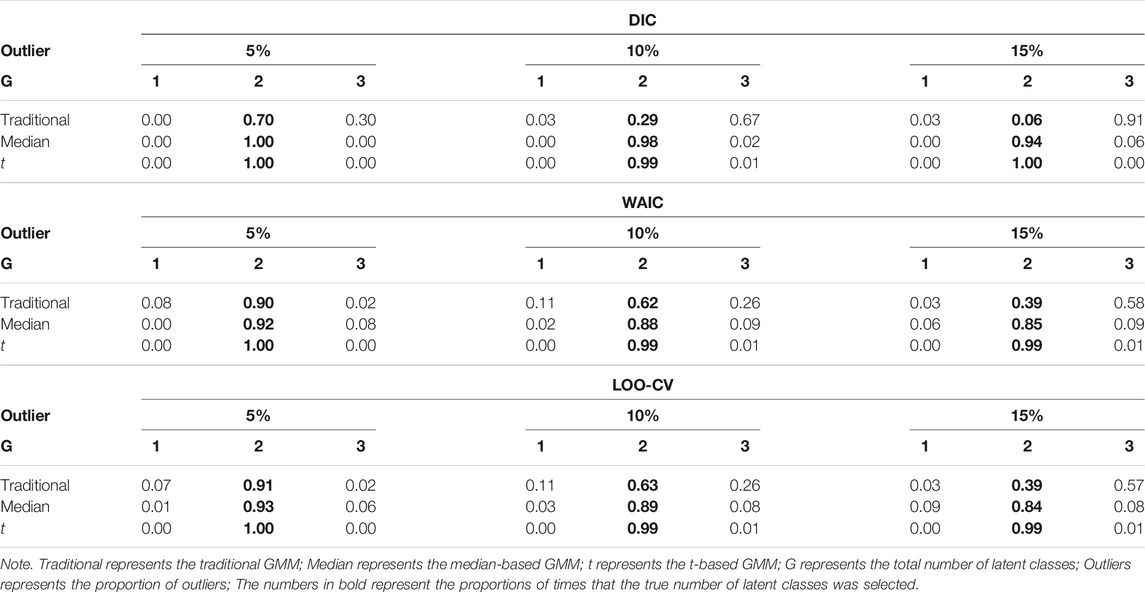
TABLE 5. Proportion for selecting 1-class, 2-class, and 3-class models using DIC, WAIC, and LOO-CV when N = 500.

Figure 3 presents the magnitude of absolute bias in the intercept and slope parameter estimates for all conditions when the number of latent classes was the same as the data generating model. The absolute bias values in Figure 3 were obtained in the way described in Study 1. The results for the conditions without outliers (i.e., r0) were included in this figure as a benchmark. As the percentage of outliers increased, the absolute bias for the traditional GMM clearly increased. The median-based and t-based GMMs also had the increasing trend as the percentage of outliers increased, but the magnitude was minor compared to the traditional GMM. The t-based GMM appeared to have a slightly higher bias than the median-based GMM when data contained outliers. The estimation results for the variance-covariance components had similar patterns.

FIGURE 3

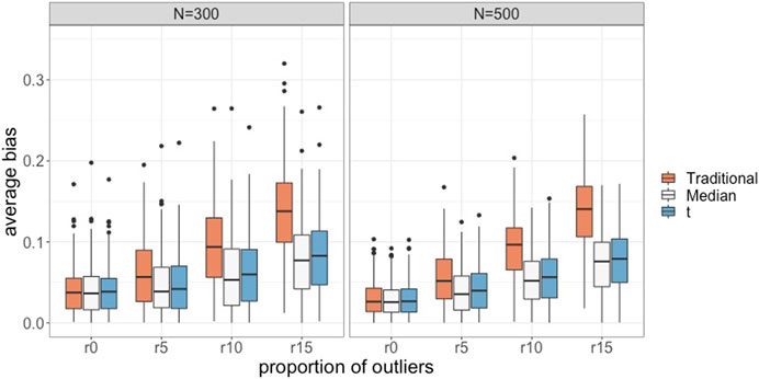
FIGURE 3. Average absolute bias for the traditional, the median-based, and the t-based GMM in conditions with varied proportions of outliers and sample sizes.

6 Conclusion and Discussion

Identifying the correct number of latent classes is one of the important tasks in growth mixture modeling analysis. It is well known that traditional growth mixture models do not perform well when data do not follow a normal distribution within each class. It may provide biased parameter estimates and detect spurious latent classes that do not have any substantive meanings. In this article, we evaluated the performance of median-based GMM in identifying the correct number of latent classes and compared it to the performance of traditional GMM and t-based GMM. The median-based GMM is known to be robust to nonnormal data, but there had been little known about how it determined the number of latent classes. We focused on situations in which data were contaminated by outliers and compared the performance of the three types of growth mixture models in identifying the number of latent classes. We used Bayesian methods for this study, and the number of latent classes was determined by DIC, WAIC, and LOO-CV. When data satisfied the normality assumption, the three growth mixture models had similar performance. Model selection accuracy was influenced by the magnitude of class separation and sample size. DIC appeared to have slightly higher accuracy than WAIC and LOO-CV, especially under the lower level of class separation. When data had outliers, class enumeration in the traditional GMM was greatly affected, and the model selection accuracy dropped as the proportion of outliers increased. In this particular situation, WAIC and LOO-CV tended to have higher accuracy than DIC. In the median-based GMM, DIC had higher accuracy than WAIC and LOO-CV. The median-based GMM also had accuracy that slightly decreased as the proportion of outliers increased or sample size decreased, but the accuracy was still high (e.g., above 0.87 by DIC across all conditions). The t-based GMM had slightly higher accuracy than the median-based GMM as the proportion of outliers increased, but the difference in accuracy decreased as sample size increased.

Finite mixture modeling is mainly used for two purposes: one is to identify latent groups of individuals that have qualitatively distinct features, and the other is to approximate a complicated distribution (Titterington et al., 1985; Bauer and Curran, 2003; Gelman et al., 2013). In our simulation study with outlying observations, it may be reasonable that the model comparison criteria used in the traditional GMM preferred the three-class model over the two-class model (the data generating model) to accommodate extreme values, especially when there were a large sample size (i.e., N = 500) and a high percentage of outliers (i.e., 15%). This behavior of traditional GMM is well documented in other studies (e.g., Bauer and Curran, 2003; Muthén and Asparouhov, 2015; Guerra-Peña and Steinley, 2016). In practice, however, researchers often conduct a growth mixture modeling analysis to discover meaningful latent classes, rather than discovering latent classes just to approximate data. In such case, using a traditional GMM may confuse researchers in determining the number of latent classes and interpretation of results. Additionally, if a relatively large number of observations (e.g., 15% when sample size is 500) were generated from a distribution that is different from the rest of the data, this portion of data would be fair to form a separate class. Outliers in our simulation study, however, were randomly generated from three different distributions rather than just one distribution. In reality, outliers may be purely random numbers independently generated from different distributions, and it would not be able to treat them as a separate class.

Both the median-based GMM and t-based GMM had high model selection accuracy when outliers exist in data. The t-based GMM had slightly higher accuracy than the median-based GMM, but the average absolute bias of intercept and slope parameter estimates for the t-based GMM was also slightly higher than the median-based GMM. This study focused on situations in which nonnormality was caused by outliers in measurement errors. Although robust methods based on Student’s t distributions may break down for skewed data, they typically perform well for data with outliers (Zhang et al., 2013). Median-based GMM is expected to perform well for other types of nonnormal data. We additionally investigated the relationship between class membership recovery and the proportion of outliers using the data generating model to examine whether the proportion of outliers influenced the class membership recovery and, consequently, parameter estimation. Given the well-separated latent classes in Study 2, the class recovery rates for the three types of GMMs were quite high. The recovery rate for the traditional GMM appeared to be influenced by the proportion of outliers (ranged from 88.1 to 93.9%). The median-based and t-based GMMs had similar class recovery rates (approximately 0.94) across all conditions. These results suggest that the bias is more likely to be associated with how each model handles outlying observations. It is worth evaluating both t- and median-based GMMs under various types of nonnormal data and providing general guidelines for robust growth mixture modeling analysis.

This study used marginal likelihoods to calculate DIC, WAIC, and LOO-CV. In a Bayesian latent variable modeling analysis, the conditional likelihood is relatively easier to obtain than the marginal likelihood because it does not require integration and is readily available in many Bayesian software programs, such as JAGS, OpenBUGS, and Stan. However, in recent studies (e.g., Merkle et al., 2019; Zhang et al., 2019), it is reported that employing the conditional likelihood in model selection can be misleading. Merkle et al. (2019) recommended use of marginal likelihood based information criteria in Bayesian latent variable analysis. In our pilot study with conditional likelihoods, DIC, WAIC, and LOO-CV performed poorly in model selection compared to their marginal likelihood counterparts. There are no systematic evaluations about the performance of conditional likelihood based information criteria and marginal likelihood based information criteria in Bayesian growth mixture modeling. This topic will be further investigated in our future research.

This article shows that median-based GMM has many advantages over traditional GMM not only in model estimation, but also in model selection. This study also compared the performance of the median-based GMM with t-based GMM, which is also known to be a robust approach to growth mixture modeling. Although the t-based GMM had higher model selection accuracy when data had outliers, the median-based GMM also achieved satisfying accuracy, especially when the model selection was evaluated by DIC. Additionally, the median-based GMM appeared to be slightly better in parameter estimation. In conclusion, we recommend the median-based GMM for growth mixture modeling analysis as it provides stable class enumeration, robust parameter estimates, and straightforward interpretation.

Data Availability Statement

The raw data supporting the conclusions of this article will be made available by the authors, without undue reservation.

Author Contributions

All authors contributed to the article.

Funding

This paper is based upon work supported by the National Science Foundation under grant no. SES-1951038.

Conflict of Interest

The authors declare that the research was conducted in the absence of any commercial or financial relationships that could be construed as a potential conflict of interest.

Footnotes

¹Mahalanobis distance was calculated as $MD=\sqrt{{\left({\mu }_1-{\mu }_2\right)}^T{\text{Σ}}^{-1}\left({\mu }_1-{\mu }_2\right)}$, where ${\mu }_1$and ${\mu }_2$ represents the mean of the first and second latent classes, respectively, and $\text{Σ}$ is the common variance-covariance matrix of latent factors.

References

Bauer, D. J., and Curran, P. J. (2003). Distributional assumptions of growth mixture models: implications for overextraction of latent trajectory classes. Psychol. Methods 8, 338–363. doi:10.1037/1082-989X.8.3.338

PubMed Abstract | CrossRef Full Text | Google Scholar

Bauer, D. J. (2007). Observations on the use of growth mixture models in psychological research. Multivariate Behav. Res. 42, 757–786. doi:10.1080/00273170701710338

CrossRef Full Text | Google Scholar

Bollen, K. A., and Curran, P. J. (2006). Latent curve models: a structural equation perspective. Hoboken, NJ: John Wiley & Sons, Vol. 467.

Google Scholar

Cain, M. K., Zhang, Z., and Yuan, K.-H. (2017). Univariate and multivariate skewness and kurtosis for measuring nonnormality: prevalence, influence and estimation. Behav. Res. Methods 49, 1716–1735. doi:10.3758/s13428-016-0814-1

PubMed Abstract | CrossRef Full Text | Google Scholar

Celeux, G., Forbes, F., Robert, C. P., and Titterington, D. M. (2006). Deviance information criteria for missing data models. Bayesian Anal. 1, 651–673. doi:10.1214/06-BA122

CrossRef Full Text | Google Scholar

Depaoli, S., Winter, S. D., Lai, K., and Guerra-Peña, K. (2019). Implementing continuous non-normal skewed distributions in latent growth mixture modeling: an assessment of specification errors and class enumeration. Multivar. Behav. Res. 54 (6), 795–821. doi:10.1080/00273171.2019.1593813

CrossRef Full Text | Google Scholar

Gelman, A., Carlin, J. B., Stern, H. S., Dunson, D. B., Vehtari, A., and Rubin, D. B. (2013). Bayesian data analysis. Boca Raton, FL: Chapman and Hall/CRC.

Google Scholar

Geraci, M., and Bottai, M. (2007). Quantile regression for longitudinal data using the asymmetric laplace distribution. Biostatistics 8, 140–154. doi:10.1093/biostatistics/kxj039

PubMed Abstract | CrossRef Full Text | Google Scholar

Geweke, J. (1991). “Evaluating the accuracy of sampling-based approaches to the calculation of posterior moments,” in Bayesian statistics 4. Editors J. M. Bernardo, J. O. Berger, A. P. Dawid, and A. F. M. Smith (Oxford: Clarendon Press), 169–193.

Google Scholar

Guerra-Peña, K., García-Batista, Z. E., Depaoli, S., and Garrido, L. E. (2020). Class enumeration false positive in skew-t family of continuous growth mixture models. PLoS One 15, e0231525. doi:10.1371/journal.pone.0231525

PubMed Abstract | CrossRef Full Text | Google Scholar

Guerra-Peña, K., and Steinley, D. (2016). Extracting spurious latent classes in growth mixture modeling with nonnormal errors. Educ. Psychol. Meas. 76, 933–953. doi:10.1177/0013164416633735

PubMed Abstract | CrossRef Full Text | Google Scholar

Kotz, S., and Nadarajah, S. (2004). Multivariate t-distributions and their applications. Cambridge, UK: Cambridge University Press.

Google Scholar

Lee, S.-Y. (2007). Structural equation modeling: a Bayesian approach. Chichester, England: John Wiley & Sons.

CrossRef Full Text | Google Scholar

Lu, Z. L., Zhang, Z., and Lubke, G. (2011). Bayesian inference for growth mixture models with latent class dependent missing data. Multiv. Behav. Res. 46, 567–597. doi:10.1080/00273171.2011.589261

CrossRef Full Text | Google Scholar

Lu, Z. L., and Zhang, Z. (2014). Robust growth mixture models with non-ignorable missingness: models, estimation, selection, and application. Comput. Stat. Data Anal. 71, 220–240. doi:10.1016/j.csda.2013.07.036

CrossRef Full Text | Google Scholar

Lubke, G., and Neale, M. C. (2006). Distinguishing between latent classes and continuous factors: resolution by maximum likelihood?. Multiv. Behav. Res. 41, 499–532. doi:10.1207/s15327906mbr4104\_4

CrossRef Full Text | Google Scholar

Lunn, D., Jackson, C., Best, N., Thomas, A., and Spiegelhalter, D. (2012). The BUGS book: a practical introduction to Bayesian analysis. Boca Raton, FL: Chapman & Hall/CRC.

Google Scholar

McLachlan, G. J. (1987). On bootstrapping the likelihood ratio test statistic for the number of components in a normal mixture. Appl. Stat. 36, 318–324. doi:10.2307/2347790

CrossRef Full Text | Google Scholar

McLachlan, G. J., and Peel, D. (2000). Finite mixture models. New York, NY: John Wiley & Sons.

CrossRef Full Text | Google Scholar

Meredith, W., and Tisak, J. (1990). Latent curve analysis. Psychometrika. 55, 107–122. doi:10.1007/BF02294746

CrossRef Full Text | Google Scholar

Merkle, E. C., Furr, D., and Rabe-Hesketh, S. (2019). Bayesian comparison of latent variable models: conditional versus marginal likelihoods. Psychometrika 84, 802–829. doi:10.1007/s11336-019-09679-0

PubMed Abstract | CrossRef Full Text | Google Scholar

Micceri, T. (1989). The unicorn, the normal curve, and other improbable creatures. Psychol. Bull. 105, 156–166. doi:10.1037/0033-2909.105.1.156

CrossRef Full Text | Google Scholar

Muthén, B., and Asparouhov, T. (2015). Growth mixture modeling with non-normal distributions. Stat. Med. 34, 1041–1058. doi:10.1002/sim.6388

PubMed Abstract | CrossRef Full Text | Google Scholar

Narasimhan, B., Johnson, S. G., Hahn, T., Bouvier, A., and Kiêu, K. (2020). Cubature: adaptive multivariate integration over hypercubes. R package version 2.0.4.1. Available at: https://cran.r-project.org/web/packages/cubature

Google Scholar

Nylund, K. L., Asparouhov, T., and Muthén, B. O. (2007). Deciding on the number of classes in latent class analysis and growth mixture modeling: a Monte Carlo simulation study. Struct. Equ. Model. A Multidiscip. J. 14, 535–569. doi:10.1080/10705510701575396

CrossRef Full Text | Google Scholar

Peugh, J., and Fan, X. (2012). How well does growth mixture modeling identify heterogeneous growth trajectories? a simulation study examining gmm’s performance characteristics. Struct. Equ. Model. A Multidiscip. J. 19, 204–226. doi:10.1080/10705511.2012.659618

CrossRef Full Text | Google Scholar

Plummer, M. (2017). JAGS Version 4.3. 0 user manual. Available at: https://sourceforge.net/projects/mcmc-jags/files/Manuals/4.x/jags_user_manual.pdf

Google Scholar

R Core Team (2019). R: a language and environment for statistical computing. Vienna, Austria: R Foundation for Statistical Computing.

Google Scholar

Schwarz, G. (1978). Estimating the dimension of a model. Ann. Stat. 6, 461–464.

CrossRef Full Text | Google Scholar

Spiegelhalter, D. J., Best, N. G., Carlin, B. P., and Van Der Linde, A. (2002). Bayesian measures of model complexity and fit. J. Roy. Stat. Soc. B. 64, 583–639. doi:10.1111/1467-9868.00353

CrossRef Full Text | Google Scholar

Titterington, D. M., Smith, A. F., and Makov, U. E. (1985). Statistical analysis of finite mixture distributions. Chichester, UK: Wiley.

Google Scholar

Tofighi, D., and Enders, C. K. (2008). “Identifying the correct number of classes in growth mixture models,”in Advances in latent variable mixture models. Editors G. R. Hancock, and K. M. Samuelson (Charlotte, NC: Information Age), 317–341.

Google Scholar

Tong, X., Zhang, T., and Zhou, J. (2020). Robust bayesian growth curve modelling using conditional medians. Br. J. Math. Stat. Psychol. [Epub ahead of print]. doi:10.1111/bmsp.1221

CrossRef Full Text | Google Scholar

Tong, X., and Zhang, Z. (2012). Diagnostics of robust growth curve modeling using student’s t distribution. Multiv. Behav. Res. 47, 493–518. doi:10.1080/00273171.2012.692614

CrossRef Full Text | Google Scholar

Vehtari, A., Gelman, A., and Gabry, J. (2017). Practical bayesian model evaluation using leave-one-out cross-validation and waic. Stat. Comput. 27, 1413–1432. doi:10.1007/s11222-016-9696-4

CrossRef Full Text | Google Scholar

Vehtari, A., Gabry, J., Magnusson, M., Yao, Y., and Gelman, A. (2019). loo: efficient leave-one-out cross-validation and WAIC for Bayesian models. R package version 2.2. Available at: https://cran.r-project.org/web/packages/loo/index.html

Google Scholar

Watanabe, S. (2010). Asymptotic equivalence of bayes cross validation and widely applicable information criterion in singular learning theory. J. Mach. Learn. Res. 11, 3571–3594.

Google Scholar

Yi, G. Y., and He, W. (2009). Median regression models for longitudinal data with dropouts. Biometrics 65, 618–625. doi:10.1111/j.1541-0420.2008.01105.x

PubMed Abstract | CrossRef Full Text | Google Scholar

Yu, K., and Moyeed, R. A. (2001). Bayesian quantile regression. Stat. Probab. Lett. 54, 437–447. doi:10.1016/S0167-7152(01)00124-9

CrossRef Full Text | Google Scholar

Zhang, X., Tao, J., Wang, C., and Shi, N.-Z. (2019). Bayesian model selection methods for multilevel irt models: a comparison of five dic-based indices. J. Educ. Meas. 56, 3–27. doi:10.1111/jedm.12197

CrossRef Full Text | Google Scholar

Zhang, Z., Lai, K., Lu, Z., and Tong, X. (2013). Bayesian inference and application of robust growth curve models using student’s t distribution. Struct. Equ. Model. A Multidiscip J. 20, 47–78. doi:10.1080/10705511.2013.742382

CrossRef Full Text | Google Scholar

Zhang, Z. (2016). Modeling error distributions of growth curve models through bayesian methods. Behav. Res. Methods 48, 427–444. doi:10.3758/s13428-015-0589-9

PubMed Abstract | CrossRef Full Text | Google Scholar