Contribution of Model Predictive Control in the Integration of Renewable Energy Sources within the Built Environment

1. Introduction

The building infrastructure represents the largest energy consumption sector in Switzerland; its share of the inland final energy consumption (FEC) amounts to nearly 43% while 86% of this consumption is solely dedicated toward space heating and domestic hot water preparation (Prognos et al., 2016). Similar values can be observed in the European Union region where built environment is responsible for over 40% of the member states FEC (Statistical Office of the European Communities, 2015) and thus represents a crucial factor within the context of sustainable development. In the view of achieving their long-term energy strategy targets such as curbing greenhouse gas emissions, improving the security of supply, and decreasing energy utilization, governments are increasingly imposing more strict performance requirements on novel and refurbished dwellings.

In the light of such legislation, modern building energy systems (BES) are facing a progressive growth in complexity, thus rendering their proper design and strategic operation increasingly compelling. While past energy systems commonly comprise a single, simple conversion unit to satisfy all thermal demands, novel configurations should include multiple conventional and renewable-based utilities to meet the strict performance criteria. However, the commonly applied two-point regulation and design methods are struggling to cope with the resulting size in decision variables. The introduction of mathematical programming techniques in BES provides an interesting approach to face the former issues; by applying model predictive control (MPC) to a holistic energy system framework, optimal solutions can indeed be generated given a specific objective and system constraints. Among the latter, the strong interaction between the BES and the local distribution power network is of major importance in regard to the flexibility the BES might be able to offer to the grid management system. Indeed, compared with non-predictive control methods, MPC is able to anticipate future generation and consumption profiles and shift controllable loads accordingly to increase self-consumption or decrease the building impact on the grid (Ashouri et al., 2015).

1.1. State-of-the-Art

Considering the growing interests in curbing the environmental impacts related to the provision of domestic service requirements, the problem of optimal sizing and operation of BES has been widely addressed in the literature. Over a decade ago, Weber et al. (2006) proposed an integrated framework to design and schedule urban energy systems at the district scale. The authors’ method relied on a bi-level optimization strategy, decomposing the problem formulation into two distinct levels; an upper realizing the system design and a lower performing the utility scheduling. This approach has been successfully applied at the building level by Collazos et al. (2009) to properly size an advanced thermal energy system for a single-family house. In their work, the authors subsequently developed an MPC controller integrating a micro-cogeneration engine, showing the benefit of deploying the controller when subjected to variable electricity tariffs for different problem formulations.

In more recent studies, Ashouri et al. (2013) proposed a holistic approach to simultaneously solve the optimal design and scheduling of BES for large, commercial dwellings. Their investigations showed the ability of the defined MILP problem formulation to cope with multiple system constraints while remaining tractable. Fux et al. (2013) applied a bi-level optimization framework, to assess optimal trade-off BES configurations for stand-alone dwellings. After defining the different designs, the authors compared their system performances when being operating using MPC and rule-based control (RBC). In the context of MILP formulations, Schütz et al. (2017) presented a BES optimization framework for residential dwellings including the discrete decision variables related to the envelope refurbishment while Wakui and Yokoyama (2015) defined a decomposition method comprising advanced, control-oriented unit models. To cope with the computational complexity of their problems, both studies solely considered several, empirically defined, typical operating periods.

From a purely control point of view, several researchers such as Oldewurtel et al. (2011) studied the effect of dynamic tariffs in reducing peak power demands for residential and office buildings though the means of MPC. The authors evaluated the potential for different scenarios, using a priori defined electrical storage sizes and envelope capacities before applying their method to the city of Zurich. De Coninck and Helsen (2016) developed and subsequently applied a non-linear MPC formulation to a heat pump powered commercial building in Brussels. Their results demonstrated the predictive regulator ability in decreasing daily energy costs while improving occupants’ comfort when compared with a standard RBC scheme. Finally, Zhao et al. (2015) presented the performance achieved using an integrated, non-linear MPC algorithm based on First Law models. By comparing various grid interaction scenarios, the authors show that substantial economic benefit can be achieved while decreasing the environmental BES impact.

Although the previous studies have successfully targeted the issue of optimal BES sizing and control, a formal definition of the potential impact of MPC within the context of building energy systems is still lacking, including answers to questions such as “to which extent does MPC improve the integration of renewable energy systems in buildings?” as well as “how can the energy system design be adapted to further increase the former share?” Indeed, the use of MPC transforms the BES into a virtual electrical storage unit with respect to standard operation techniques by shifting controllable loads to reduce the operational costs. In view of the different system boundary conditions, MPC might considerably increase the self-consumption of on-site generated power, such as from photovoltaic panels or combined heat and power units, while respecting the different service requirements, grid interactions, and utility integration constraints. Hence, this study attempts to contribute to the state-of-the-art by proposing a systematic method to provide a first answer to the aforementioned questions. The following study is an extension of the authors’ previous work presented in Stadler et al. (2017b); while the systematic approach and geographical clustering have been introduced in the former paper, the novel further comprises an advanced formulation of the considered performance indicators, additional devices in the modeling framework as well as a multi-objective national assessment of optimal BES designs.

The structure of this article is the following: Section 2 describes the developed method, and Section 3 defines the case study considered. Section 4 exposes the resulting advantages of applying predictive control in buildings, while Section 5 finally provides concluding comments about the proposed approach and relevant findings of this study.

2. Materials and Methods

This study proposes a systematic approach to evaluate both the local and national contribution of model predictive control (MPC) techniques in integrating modern complex energy systems in the Swiss building stock. As illustrated in Figure 1, the developed method comprises three major steps which are detailed in the following section:

1. The data reduction step (section 2.1) in which the problem size is drastically decreased to improve both the problem tractability and solvability.

2. The optimization step (section 2.2) in which the optimal sizing and/or control problem is systematically solved for different operational constraints and boundary conditions.

3. The post-processing step (section 2.3) in which the solutions of previous step are analyzed to provide optimal trade-off solutions to stakeholders.

FIGURE 1

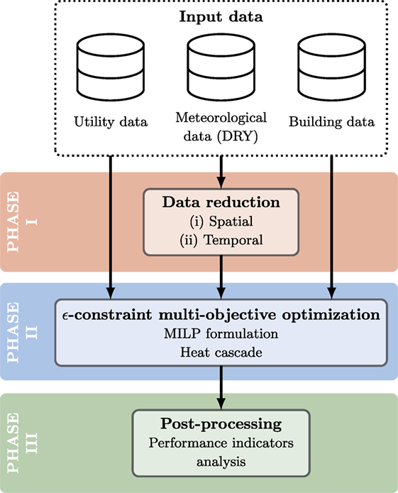
Figure 1. Illustration of the developed methods.

2.1. Data Reduction

The initial input data consist of the national building register (RegBL; Section Bâtiments et logements, 2015), which comprises generic information on around 1.6 mio dwellings such as their category, age, and size. In view of the latter number, an individual assessment at this scale is completely intractable while requiring a tremendous computational effort. Thus, a first data reduction step is performed. Indeed, given the available data¹ and the classification results presented in Girardin et al. (2010), three specific building types have been defined and analyzed throughout the following study; a single-family house, an apartment block, and a mixed use building (Stadler et al., 2017b), each of them comprising nine subcategories regarding their construction period. In regard to the approach of Girardin et al. (2010), space heating demands are characterized on the basis of the heating curve definition while purely affectation-specific requirements (e.g., power and domestic hot water needs) are evaluated using standards of the Swiss society of engineers and architects (SIA 2024, 2015). Since these different building types are obviously subject to different climatic conditions throughout the year depending on their location on the national territory, an additional data reduction step is required to group similar demand regions: spatial clustering.

2.1.1. Spatial Clustering

Spatial data reduction aims at identifying typical geographical regions with identical climatic conditions (i.e., space heating demands). The applied approach relies on a modified procedure initially proposed by Fazlollahi et al. (2014) and uses a specific implementation of the k-medoids technique: mixed-integer linear programming (MILP). This clustering method defines the cluster centers from the initial data set based on the smallest sum of squared distances within each cluster. At the clustering level, the k-medoid appears to provide more robust results than the commonly applied k-means technique as discussed by Kaufman and Rousseeuw (2009) and recently noticed in the comparative study of Schütze et al. (2016). In this study, the considered input data can be described as follows:

• The initial observations i consist of the 2,441 different communes territories of Switzerland. Indeed, buildings located within a same commune have been considered exposed to identical climatic conditions and hence, clustered a priori within those territories. The national building stock can thus be directly clustered at the commune scale.

• The commune attributes a include the number of heating (HDD) and cooling (CDD) degree days as well as the annual global horizontal irradiance (GHI) related to the ith hourly of the design reference year (DRY) profile. Indeed, in urban energy system planning, building performances are commonly assessed by means of normalized DRY (SIA 2028, 2008). These hourly profiles are constructed from historical meteorological measurements and incorporate typical climatic conditions arising at the location of interest. The annual cyclicity of the former climatic states supports the assumption of considering the weather data as constant over the entire equipment lifetime, hence decreasing the temporal simulation scope from about 20^years ×8760^hours to 1^years ×8760^hours time steps. The definitions of these parameters are hence expressed in equations (1)–(3) where the index d represents a day and ${\overline{\text{T}}}^{\mathit{amb}}$ the mean daily ambient temperature (European Environment Agency, 2012)

${\text{HDD}}_i={\displaystyle \sum _{d=1}^{365}}\left(18-{\overline{\text{T}}}_{i,d}^{\mathit{amb}}\right)\forall {\overline{\text{T}}}_{i,d}^{\mathit{amb}}\le 15$ (1)

${\text{CDD}}_i={\displaystyle \sum _{d=1}^{365}}\left({\overline{\text{T}}}_{i,d}^{\mathit{amb}}-18\right)\forall {\overline{\text{T}}}_{i,d}^{\mathit{amb}}\ge 18.3$ (2)

${\text{GHI}}_i={\displaystyle \sum _{d=1}^{365}}{\text{GHI}}_{i,d}$ (3)

To assess the different attributes a of each observation i, the available data of 40 national weather stations have been extended by using the inverse distance squared interpolation method introduced by Shepard (1968) and further extended by Lefèvre et al. (2002). However, to properly assess the annual load profiles of the different cluster centers a posteriori, the medoids locations are constraint in the MILP problem formulation to the latter weather stations. Following the computation, the optimal cluster size has finally been selected with respect to a single-performance indicator:

• The silhouette index (S) measures the cluster cohesions in comparison with their separations. The index ranges from −1 to 1, large values representing a good cluster structure while low and negative values reflect a weak configuration. Hence, the indicator should be maximized during the selection process.

To guarantee a reliable representation of the original data by the reduced data space, a minimum acceptable number of clusters are defined on the basis of two quality indicators:

• The error in load duration curve (ELDC) of attribute a (Domínguez-Muñoz et al., 2011) indicates the global (national) SD of the original and clustered load curves.

• The mean profile deviation (σ_cdc) of attribute a (Fazlollahi et al., 2014) evaluates the difference between the observations (commune) and their representative cluster medoid.

Figure 2 presents the evolution of the different indicators with respect to the cluster number n_k. The highest values of the average silhouette index are observed for n_k = 2, n_k = 3, and n_k = 4 zones while both the errors in load duration curves as well as the mean profile deviations continuously decrease with the rise in n_k. The minimum acceptable number $n_k^{\text{min}}$ of cluster is assessed through an improvement threshold ϵ in quality indicators resulting from increasing the cluster size from k to k + 1; hence, considering a value of ϵ = 0.20 (Fazlollahi et al., 2014), the resulting $n_k^{\text{min}}=5$. In view of this lower bound, the next local performance indicator maximum is n_k = 7, and thus the following climatic region number has been selected.

FIGURE 2

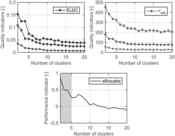
Figure 2. Spatial data reduction quality indicators for heating degree days (diamond), global horizontal irradiance (star), cooling degree days (circle), and performance indicator.

The spatial cluster layout resulting from the aforementioned algorithm is illustrated in Figure 3. As expected, the different geographical topologies of the communes are well reflected within the assessed partition: (i) the Alps (south and east), (ii) the Plateau (west and the north-east), and (iii) the Jura (north-west). Consequently, in addition to the previously discussed statistical quality indicators, the figure provides a good graphical validation of the selected cluster size. Finally, Table 1 provides aggregated overview of the average attributes and annual service requirements of each climatic zones.

FIGURE 3

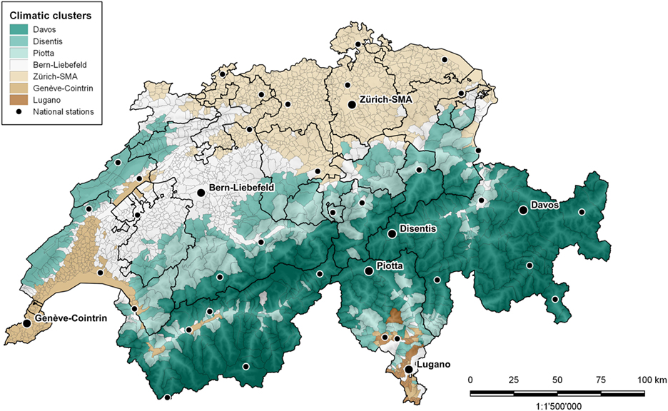
Figure 3. Identified climatic zones in Switzerland.

TABLE 1

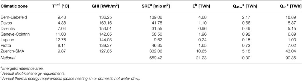
Table 1. Annual demand and climatic conditions.

2.1.2. Temporal Clustering

Although the preceding steps drastically decreased the problem size from around 1.6 mio to 3^types × 9^age × 7^zones dwellings, a last data reduction operation is finally performed prior solving the optimization problem to further decrease the remaining computational complexity: temporal clustering. Thereafter, the approach introduced in the previous section (section 2.1.1) is anew applied to identify a set of typical days for each spatial cluster. Indeed, similar to the equipment lifetime, a DRY might be represented by a series of daily climatic patterns with certain probability of occurrence. The considered input data of the temporal clustering problem can be described as follows:

• The initial observations i are the 365 days of the DRY.

• The attributes a consist of 24 measurements (hours) of the ambient temperature and the global horizontal irradiance. Additional temporal data such as electricity and hot water demand profiles have been assessed from the standard values of Swiss Society of Engineers and Architects (SIA 2024, 2015) and thus have not been considered in the following process step.

Since in the temporal data reduction step the observation i comprises multiple measurements, an additional quality indicator is implemented:

• The profile deviation (σ_profile) of attribute a (Fazlollahi et al., 2014) evaluates the SDs between the original and typical profiles with respect to their averages.

In the case of the Geneva-Cointrin climatic zone, the highest values of the average silhouette index are observed for n_k = 2, n_k = 4, and n_k = 3 periods while the quality indicators tend to decrease with the increase in n_k (Figure 4). Considering a threshold value ϵ = 0.12, the minimum acceptable cluster size is $n_k^{\text{min}}=7$ and consequently, n_k = 8 has finally been chosen as the best trade-off solution. The temporal scope of the optimization problem is thus reduced from 1^years ×8760^hours to 8^days ×24^hours time steps.

FIGURE 4

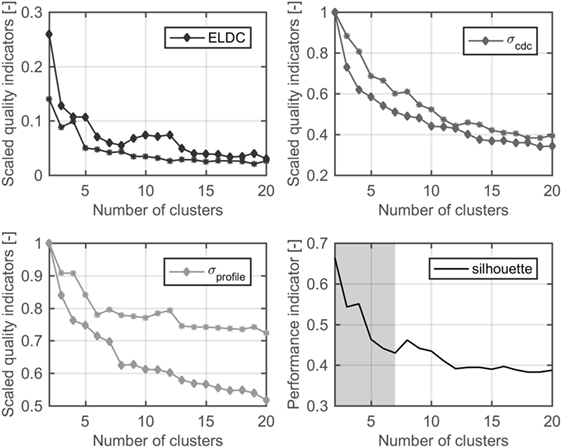
Figure 4. Temporal data reduction quality indicators for global horizontal irradiance (diamond), ambient temperature (star), and performance indicator of Geneva-Cointrin.

Figure 5 represents the original DRY profiles of both attributes in addition of the load duration curves of both the original data and the respective typical days. As observed, the latter graph provides a good visual validation of the selected clusters (Rager, 2015). Additional information on the remaining (6) typical climatic regions are provided in Stadler et al. (2017a).

FIGURE 5

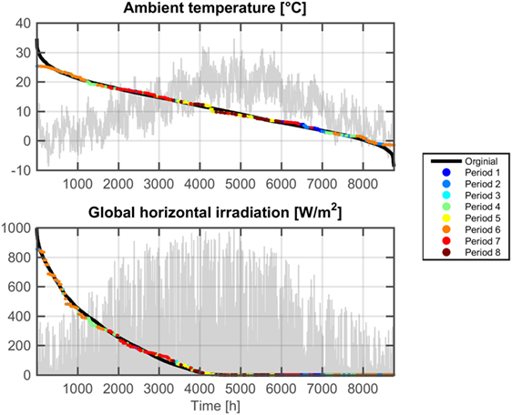
Figure 5. The ambient temperature and solar irradiation DRY load duration curves (black, front) and profiles (gray, background) of Geneva-Cointrin represented by 8 typical periods (colored).

2.2. System Optimization

This section presents the different optimization problem formulations applied in the proposed method. In the following definitions, parameters are represented by standard roman text letters, variables by italic text letters and sets by bold text letters. The sets implemented throughout this section are defined as follows; the set U includes all utility technologies considered in the pseudo-superstructure (Figure 6) while the set P comprises the different typical operating periods defined in Section 2.1.2. The set T refers to the hourly discrete time steps of each period; T ∈ [1, 24]. Finally, regarding the convention proposed by Borel and Favrat (2010), the index + denotes an incoming flow while − indicates an outgoing flow.

FIGURE 6

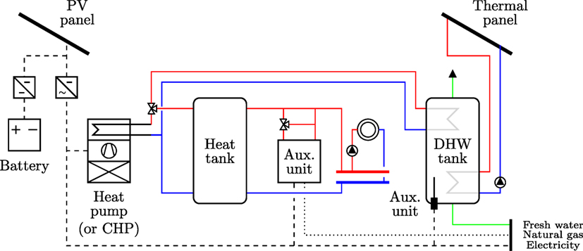
Figure 6. Energy system pseudo-superstructure (Stadler et al., 2017b).

2.2.1. Design and Scheduling Under MPC

This study applies an ϵ-constraint multi-objective optimization approach (Mavrotas, 2009) to simultaneously evaluate the optimal design and schedule of building energy systems. The problem is implemented using a mixed-integer linear programming (MILP) technique to solve the set of static and first-order linear differential equations of the building and different utility models. The latter formulation has indeed been identified as a proper choice to describe both the logical and continuous behavior inherent to energy systems (Bemporad and Morari, 1999). The use of mixed-integer non-linear programming (MINLP) remains a non-trivial task as discussed by Grossmann (2012); indeed, while improving the model precision, the latter formulation reflects a poor robustness due to the initial point issue when solving each relaxed sub-problem. Therefore, practitioners tend to reformulate the problem as an MILP by discretizing non-linear behaviors as implemented in the following study (e.g., heat cascade). Finally, in regard to the aforementioned temporal decomposition, the optimal device scheduling can be considered as a building controller applying MPC with a daily time horizon and perfect load and input predictions.

2.2.1.1. Objective Functions

The main problem objective is the minimization of the annual building operating expenses, which comprise both the natural gas and power grid exchanges. The former are defined in equation (4) where op refers to the grid energy tariffs, $\dot{E}$ to the electrical power flows, $\dot{H}$ to the chemical–natural gas–power flows, d to the indexed time step duration, and Σ the set of decision variables reported in Stadler et al. (2017a)

$\begin{array}{l}\hfill \underset{\Sigma }{\min }{\displaystyle \sum _{p=1}^{\mathit{\text{P}}}}{\displaystyle \sum _{t=1}^{\mathit{\text{T}}}}\left({\text{op}}_{p,t}^{\mathit{el},+}\cdot {\dot{E}}_{\text{grid},p,t}^{+}-{\text{op}}_{p,t}^{\mathit{el},-}\cdot {\dot{E}}_{\text{grid},p,t}^{-}+{\text{op}}_{p,t}^{\mathit{ng},+}\cdot {\dot{H}}_{\text{grid},p,t}^{+}\right)\cdot {\text{d}}_p\cdot {\text{d}}_t\hfill \\ \Sigma ={\left\{{\dot{Q}}_{\text{build},p,t,k},y_{u,p,t},{\dot{Q}}_{u,p,t,k},{\dot{E}}_{u,p,t},y_u,F_u\right\}}_{u\in \mathit{\text{U}},p\in \mathit{\text{P}},t\in \mathit{\text{T}},k\in \mathit{\text{K}}}\hfill \end{array}$ (4)

The second objective, formulated as an ϵ-constraint in the optimization problem, is the capital expenses as expressed in equation (5) where inv_{1, u} and inv_{2, u} denote the linear cost function parameters, τ the investment annualization factor, y_u the unit existence while F_u is the device sizing variable

$\frac{1}{\mathrm{\tau }}{\displaystyle \sum _{u=1}^{\mathit{\text{U}}}}\text{in}{\text{v}}_{1,u}\cdot y_u+\text{in}{\text{v}}_{2,u}\cdot F_u\le {\mathrm{ϵ}}_{\mathit{inv}}$ (5)

Finally, a third objective function—implemented as an ϵ-constraint—is used to represent the power network interests: the grid multiple (GM). As detailed in equation (6), this parameter limits the building power profile peaks ${\dot{E}}_{\text{grid}}$ with respect to the daily average demand and thus decreases the consequent stress on the distribution network from strong demand/supply surges. For the sake of readability, the total period duration is denoted by n_t = |T |

$\frac{\left({\dot{E}}_{\text{grid},p,t}^{+}-{\dot{E}}_{\text{grid},p,t}^{-}\right)}{\frac{1}{n_t}{\displaystyle \sum _{t=1}^{\mathit{\text{T}}}}\left({\dot{E}}_{\text{grid},p,t}^{+}-{\dot{E}}_{\text{grid},p,t}^{-}\right)}\le {\mathrm{ϵ}}_{\mathit{gm}}$ (6)

2.2.1.2. Heat Cascade

The heat cascade balances the system heat loads while satisfy the second law of thermodynamics. Equation (7) thus defines the thermal energy balance of each temperature interval k where ${\dot{Q}}_k^{-}$ represents the released heat of utility u_h, ${\dot{Q}}_k^{+}$ represents the heat demand of utility u_c, and ${\dot{R}}_k$ the residual heat cascaded to next interval k + 1. In addition, no heat is cascaded at the first and last intervals to ensure a closed thermal energy balance

$\begin{array}{cc}{\dot{R}}_{k,p,t}-{\dot{R}}_{k+1,p,t}={\displaystyle \sum _{u_h=1}^{\mathit{\text{U}}}}{\dot{Q}}_{u_h,k,p,t}^{-}-{\displaystyle \sum _{u_c=1}^{\mathit{\text{U}}}}{\dot{Q}}_{u_c,k,p,t}^{+}\hfill & \forall p\in \mathit{\text{P}},t\in \mathit{\text{T}},k\in \mathit{\text{K}}\hfill \\ {\dot{R}}_{1,p,t}={\dot{R}}_{n_k+1,p,t}=0\hfill & \forall p\in \mathit{\text{P}},t\in \mathit{\text{T}}\hfill \end{array}$ (7)

2.2.1.3. Energy Balances

The electrical and natural gas energy balances are defined in equation (8) where ${\dot{\text{E}}}_{\mathit{build}}^{-}$ refers to the building uncontrollable load profile

$\begin{array}{ll}{\dot{E}}_{\text{grid},p,t}^{+}+{\displaystyle \sum _{u=1}^{\mathit{\text{U}}}}{\dot{E}}_{u,p,t}^{+}={\displaystyle \sum _{u=1}^{\mathit{\text{U}}}}{\dot{E}}_{u,p,t}^{-}+{\dot{E}}_{\text{grid},p,t}^{-}+{\dot{\text{E}}}_{\text{build},p,t}^{-}\hfill & \forall p\in \mathit{\text{P}},t\in \mathit{\text{T}}\hfill \\ {\dot{H}}_{\text{grid},p,t}^{+}={\displaystyle \sum _{u=1}^{\mathit{\text{U}}}}{\dot{H}}_{u,p,t}^{-}\hfill & \forall p\in \mathit{\text{P}},t\in \mathit{\text{T}}\hfill \end{array}$ (8)

2.2.1.4. Cyclic Conditions

To prevent any energy accumulation between the different independent operating periods p, cyclic constraints (equation (9)) enforce all system states to return to their initial value at the end of each control horizon n_t = |T |. The latter constraints target the dwelling temperature T_b as well as the thermal Q and electrical energy E stored in the respective storage units. Indeed, as presented in Section 2.1.2, the typical days p represent different operating conditions with a given probability of occurrence during the system lifetime. Therefore, equation (9) is included in the problem formulation to avoid any energy bias

$\begin{array}{ll}{T}_{\text{build},p,1}=T_{\text{build},p,n_t}\hfill & {\forall }_p\in \mathit{\text{P}}\hfill \\ Q_{u,p,1}=Q_{u,p,n_t}\hfill & {\forall }_p\in \mathit{\text{P}},u\in \mathit{\text{U}}\hfill \\ E_{u,p,1}=E_{u,p,n_t}\hfill & {\forall }_p\in \mathit{\text{P}},u\in \mathit{\text{U}}\hfill \end{array}$ (9)

2.2.1.5. Unit Sizes

The unit existence y_u and logical state (on/off) y_{u, p, t} are expressed in equation (10) where ${\text{f}}_u^{\mathit{min}}$ and ${\text{f}}_u^{\mathit{min}}$ describe the device minimal and maximal sizing values, respectively

$\begin{array}{ll}{y}_u\cdot {\text{f}}_u^{\mathit{min}}\le F_u\le y_u\cdot {\text{f}}_u^{\mathit{max}}\hfill & {\forall }_u\in \mathit{\text{U}}\hfill \\ y_{u,p,t}\le y_u\hfill & {\forall }_u\in \mathit{\text{U}}\hfill \end{array}$ (10)

The different energy system units included in the presented framework are depicted in Figure 6. Although the figure solely illustrates an air–water heat pump as primary thermal conversion unit, a CHP device or a combination of multiple technologies might also be selected by the solver. To propose future, efficient energy systems to the different stakeholders, solely solid oxide (SOFC), and low temperature proton exchange membrane fuel cells (LPEM) are considered as CHP units in the following structure. In addition, it is worth noting that the final hydraulic layout (including, e.g., pumps, by-passes, three-way valves) of the designed BES may be implemented differently, according to the selected solution. Further details on the optimization problem formulation and input data are reported in Stadler et al. (2017a).

2.2.2. Scheduling Under RBC

To highlight the benefit resulting from the use of a predictive regulation (MPC) compared with a non-predictive, standard rule-based control (RBC) method, a second MILP problem formulation is proposed. The considered RBC algorithm includes standardized control methods applied in buildings such as (1) the heating curve signature approach for space heating and (2) a two-point temperature control approach for the domestic hot water tank management. The related model is based on the definition described in section 2.2.1 and hence, the following subsection solely presents the modifications from the original reference formulation.

2.2.2.1. Objectives

Similar to the previous model, the problem objective function is the minimization of operating expenses. Nevertheless, to avoid generating any arbitrage conditions (e.g., in the case of using a CHP), the feed-in tariff op⁻ is set equal to the purchasing cost op⁺. The annual energy bill is thus corrected a posteriori to be comparable to the MPC results

$\underset{\Sigma }{\text{min}}{\displaystyle \sum _{p=1}^{\mathit{\text{P}}}}{\displaystyle \sum _{t=1}^{\mathit{\text{T}}}}\left({\text{op}}_{p,t}^{\mathit{el},+}\cdot {\dot{E}}_{\text{grid},p,t}^{\prime +}-{\text{op}}_{p,t}^{\mathit{el},+}\cdot {\dot{E}}_{\text{grid},p,t}^{\prime -}+{\text{op}}_{p,t}^{\mathit{ng},+}\cdot {\dot{H}}_{\text{grid},p,t}^{\prime +}\right)\cdot {\text{d}}_p\cdot {\text{d}}_t$ (11)

2.2.2.2. Building

In RBC, the local regulator is following the predefined minimum comfort temperature during the heating period while during the cooling season, the maximum comfort bound. Hence, regarding the model formulation detailed in Stadler et al. (2017a), no additional heat can be provided or extracted in view of the minimum energy requirements (equation (12))

$\begin{array}{ll}{\dot{Q}}_{\text{build},p,t,k}^{\prime +}=0\hfill & {\forall }_k\ge 2,p\in \mathit{\text{P}},t\in \mathit{\text{T}}\hfill \\ {\dot{Q}}_{\text{build},p,t,k}^{\prime -}=0\hfill & {\forall }_k\ge 2,p\in \mathit{\text{P}},t\in \mathit{\text{T}}\hfill \end{array}$ (12)

2.2.2.3. Unit Existence

Equation (13) fixes the BES design to a previously defined optimal solution ${\text{F}}_u^{\ast }$ except for the photovoltaic array. The latter device is indeed decoupled from the building and operated off-site to prevent the solver from shifting controllable loads toward high generation periods. The electricity produced from the photovoltaic panels is then subtracted a posteriori from the building power demand while the operating expenses are corrected accordingly

$\begin{array}{ll}{F}_u^{\prime }={\text{F}}_u^{\ast }\hfill & {\forall }_u\in \mathit{\text{U}}\backslash \left\{\text{PVA}\right\}\hfill \\ F_{\text{PVA}}^{\prime }=0\hfill \end{array}$ (13)

2.2.2.4. Hot Water Tank

Since, when operating under RBC, the main role of the buffer tank is in providing thermal power during defrosting periods and limiting the number of start-up cycles, the device is solely required to follow the building return temperature, hence fixing the heat output to null (equation (14))

${\dot{Q}}_{\text{HWT},p,t}^{\prime -}=0{\forall }_p\in \mathit{\text{P}},t\in \mathit{\text{T}}$ (14)

2.2.2.5. Domestic Hot Water Tank

In RBC, the domestic hot water tank is regulated through a simple two-point control method; when reaching the lower state of charge $m_{\text{DWT}}^{\text{min}}$, the device is fully charged. Equation (15) models the latter behavior where the binary variable y_DWT refers to a charging need and the parameter M to a large value. To offload power networks, electrically powered domestic hot water tanks are typically charged during night time and thus, at t = 1 the storage unit is fully charged and operating according to the aforementioned regulation scheme

$\begin{array}{cc}{m}_{\text{DWT},p,1,n_k}^{\prime }={\text{F}}_{\text{DWT}}^{\ast }\cdot \mathrm{\rho }\hfill & \forall p\in \mathit{\text{P}}\hfill \\ \left(1-y_{\text{DWT},p,t}^{\prime }\right)\cdot {\text{m}}_{\text{DWT}}^{\text{min}}\le \left(1-{\mathrm{\sigma }}_{\text{DHW},n_k}\cdot {\text{d}}_t\right)\cdot m_{\text{DWT},p,t,n_k}^{\prime }-\left({\dot{\text{m}}}_{\text{build},p,t}\right)\cdot {\text{d}}_t\hfill & \forall p\in \mathit{\text{P}},t\in \mathit{\text{T}}\hfill \\ {\text{m}}_{\text{DWT}}^{\text{min}}+\left(1-y_{\text{DWT},p,t}^{\prime }\right)\cdot \text{M}\ge \left(1-{\mathrm{\sigma }}_{\text{DHW},n_k}\cdot {\text{d}}_t\right)\cdot m_{\text{DWT},p,t,n_k}^{\prime }-\left({\dot{\text{m}}}_{\text{build},p,t}\right)\cdot {\text{d}}_t\hfill & \forall p\in \mathit{\text{P}},t\in \mathit{\text{T}},\hfill \\ {\dot{Q}}_{\text{DWT},p,t,k}^{\prime -}\le \text{M}\cdot y_{\text{DWT},p,t}^{\prime }\hfill & \forall p\in \mathit{\text{P}},t\in \mathit{\text{T}},k\in \mathit{\text{K}}\hfill \\ m_{\text{DWT},p,t+1,n_k}^{\prime }\ge y_{\text{DWT},p,t}^{\prime }\cdot {\text{F}}_{\text{DWT}}^{\ast }\hfill & \forall p\in \mathit{\text{P}},t\in \mathit{\text{T}}\hfill \end{array}$ (15)

2.2.2.6. Battery

Similar to the photovoltaic array, the battery is decoupled from the BES during the optimization process (equation (16)) and integrate a posteriori through a simple rule control; during excess production, the battery is charged until reaching its capacity while during demand periods, the unit is discharged

$E_{\text{BAT},p,t}^{\prime }=0$ (16)

2.3. Performance Indicators

In the last process step, additional performance indicators are calculated to assess the different optimization results in view of the different stakeholders’ interests.

2.3.1. Total Annualized Expenses

The total annualized expenses (TOTEX) simply reflect the economic benefits resulting from the smart installation and operation of complex BES with renewable-based conversion utilities. As stated in equation (19), the latter are computed from the primary objective function: (i) the operating expenses and the first epsilon constraint, (ii) the annualized capital expenses

$\begin{array}{l}\text{TOTEX}={\displaystyle \sum _{p=1}^{\mathit{\text{P}}}}{\displaystyle \sum _{t=1}^{\mathit{\text{T}}}}\left({\text{op}}_{p,t}^{\mathit{el},+}\cdot {\dot{E}}_{\text{grid},p,t}^{+}-{\text{op}}_{p,t}^{\mathit{el},-}\cdot {\dot{E}}_{\text{grid},p,t}^{-}+{\text{op}}_{p,t}^{\mathit{ng},+}\cdot {\dot{H}}_{\text{grid},p,t}^{+}\right)\cdot {\text{d}}_p\cdot {\text{d}}_t\hfill \\ +\frac{1}{\mathrm{\tau }}{\displaystyle \sum _{u=1}^U}\text{in}{\text{v}}_{1,u}\cdot y_u+\text{in}{\text{v}}_{2,u}\cdot F_u\hfill \end{array}$ (17)

2.3.2. Self-Consumption and Self-Sufficiency

The self-consumption (SC) represents the ratio of the on-site generated power consumption in regard to the total produced electricity as defined in equation (20), ${\dot{E}}^{\mathit{gen}}$ and ${\dot{E}}_{\text{grid}}^{-}$ referring to the hourly generated and export power flows, respectively. The former measure, formalized by the authors of Luthander et al. (2015), reflects the system ability in shifting controllable loads toward high production periods and thus, in decreasing grid export power flows

$\text{SC}=\frac{{\displaystyle \sum _{p=1}^{\mathit{\text{P}}}}{\displaystyle \sum _{t=1}^{\mathit{\text{T}}}}\left({\dot{E}}_{p,t}^{\text{gen}}-{\dot{E}}_{\text{gird},p,t}^{-}\right)\cdot {\text{d}}_p\cdot {\text{d}}_t}{{\displaystyle \sum _{p=1}^{\mathit{\text{P}}}}{\displaystyle \sum _{t=1}^{\mathit{\text{T}}}}\left({\dot{E}}_{p,t}^{\text{gen}}\cdot {\text{d}}_p\cdot {\text{d}}_t\right)}$ (18)

The self-sufficiency (SS) on the other hand defines the ratio of the on-site generated power consumption in regard to the total electricity consumption as defined in equation (19) where ${\dot{E}}_{\text{grid}}^{+}$ denotes the hourly imported power flow. Also defined by Luthander et al. (2015), this indicator describes the degree of penetration of distributed energy systems—including renewable-based conversion utilities—with respect to the building electricity use. It is worth noting that the intersection between the self-consumption and the self-sufficiency (i.e., SC = SS) reflects the well-known net zero energy building label

$\text{SS}=\frac{{\displaystyle \sum _{p=1}^{\mathit{\text{P}}}}{\displaystyle \sum _{t=1}^{\mathit{\text{T}}}}\left({\dot{E}}_{p,t}^{\text{gen}}-{\dot{E}}_{\text{gird},p,t}^{-}\right)\cdot {\text{d}}_p\cdot {\text{d}}_t}{{\displaystyle \sum _{p=1}^{\mathit{\text{P}}}}{\displaystyle \sum _{t=1}^{\mathit{\text{T}}}}\left({\dot{E}}_{\text{gird},p,t}^{+}+{\dot{E}}_{p,t}^{\text{gen}}-{\dot{E}}_{\text{gird},p,t}^{-}\right)\cdot {\text{d}}_p\cdot {\text{d}}_t}$ (19)

2.3.3. Electrical Storage Equivalence

The change in consumption behavior resulting from the use of MPC for building energy systems can be represented, in view of the power network operator, as a virtual electrical storage capacity when compared with a conventional control method. The conservative definition of the electrical storage equivalence (ESE) introduced in the author’s previous work (Stadler et al., 2017b) has been extended to a variable, period-dependant p value. Moreover, the novel definition integrates the dynamic behavior inherent to an electrical storage unit and thus, potentially increases the exploited capacity C^ESE. Equation (20) expresses the latter indicator as follows:

$C_p^{\text{ESE}}=\underset{t\in \mathit{\text{T}}}{\mathit{max}}{\text{SOC}}_{t,p}{\forall }_p\in \mathit{\text{P}}$ (20)

where

${\text{SOC}}_{t+1,p}={\text{SOC}}_{t,p}+\left(\left({\dot{E}}_{\text{grid},p,t}^{+}-{\dot{E}}_{\text{grid},p,t}^{-}\right)-\left({\dot{E}}_{\text{grid},p,t}^{\prime +}-{\dot{E}}_{\text{grid},p,t}^{\prime -}\right)\right)\cdot {\text{d}}_t{\forall }_t\in \mathit{\text{T}},p\in \mathit{\text{P}}$ (21)

${\text{SOC}}_{n_t+1,p}={\text{SOC}}_{1,p}+{\mathrm{ϵ}}_p^{\text{ESE}}{\forall }_p\in \mathit{\text{P}}$ (22)

with SOC referring to the state of charge of the ESE. In addition, the round-trip efficiency ϵ^ESE associated with the use of the latter capacity can be determined for each period p as shown in equation (23)

${\mathrm{ϵ}}_p^{\text{ESE}}={\displaystyle \sum _{t=1}^{\mathit{\text{T}}}}\left({\dot{E}}_{\text{grid},p,t}-{\dot{E}}_{\text{grid},p,t}^{\prime }\right)\cdot {\text{d}}_t$ (23)

Figure 7 illustrates the introduced concept for two typical spring days; during day time, the penetration of renewable energy sources engenders a negative power balance while during night time the latter is positive. Nevertheless, when operating the building energy systems with MPC, the local controllers seek to shift controllable loads from low toward high generation periods to benefit from the on-site produced electricity which explains the difference in power profiles. The former change in consumption behavior might be represented as a grid operated storage system charged during positive profile difference periods (green areas) and discharged during negative ones (red area). The resulting ESE state of charge is represented by the blue curve, which nearly returns to its initial state at the end of the operating period p in view of the cyclic conditions imposed in equation (9). Indeed, the difference between SOC_{1, p} and ${\text{SOC}}_{n_t+1,p}$ (equation (22)) results from the change in daily electricity consumption and can be interpreted as the ESE round-trip efficiency ϵ^ESE. It is worth noting that the latter value might be positive or negative since the use of MPC may improve the overall system efficiency.

FIGURE 7

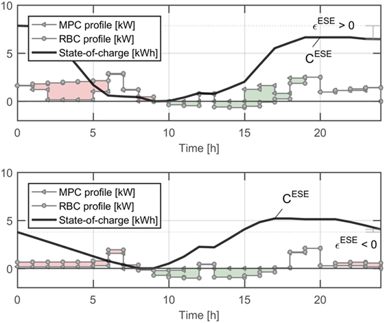
Figure 7. Building net power profiles and state of charge of the virtual battery (ESE) during typical spring days. The colored areas represent charging (green) and discharging (red) periods, respectively.

3. Results and Discussion

The following section presents the results generated by applying the proposed method to the national building stock. Prior implementing the iterative ϵ-constraint optimization approach, two base case scenarios S_i are defined as follows:

• S₀ solely includes a natural gas boiler as primary conversion unit in addition to the minimum allowable domestic hot water tank, thus representing the current fossil-fuel based BES.

• S₁ consists of an air–water heat pump as primary conversion unit, the minimum required buffer and domestic hot water tanks in addition to electrical auxiliary heaters if necessary, hence representing the minimum investment needed for a modern BES.

Starting from S₁, the ϵ-constraint problem formulation is then applied by progressively increasing the upper bound on the capital expenses, expressed as a percentage of the latter initial solution. Indeed, at each iteration, the ϵ_inv value is raised by 10% of the S₁ investment costs solution until reaching 100%, i.e., twice of the former amount. All computations are performed with the commercial solver CPLEX 12.7 on a single machine including a double core 2.4 GHz CPU and 8 GB RAM. The maximum tolerated relative optimality gap (MIP gap) is set to 0.5%.

3.1. Single-Building Level

Prior analyzing the impact of smart design and control techniques on the large scale, this subsection presents and discusses the results for different building types. Figure 8 thus depicts the Pareto fronts obtained from the ϵ-constraint multi-objective optimization formulations applied to a single-family house located in the Geneva-Cointrin climate region when applying MPC (i), RBC (ii), and MPC with an ϵ_gm bound (iii). Starting from solution S₁, the operating expenses are rapidly decreasing with the incremental increase in capital expenses for all scenarios (zones I and II); nevertheless, in the case of (i), the latter benefit levels off around 1,650 CHF/100 ⋅ m² (zone III). The comparison between the fronts (i) and (ii) shows a slight economic benefit resulting from the implementation of MPC over RBC, values rising from nearly 0% for S₀ to 5% at the end of (zone II) before dropping again for large investment thresholds (zone III). A similar behavior is observed in the case of the self-consumption, differences are growing from 0% in (zone I) to nearly 27% at the end of (zone II) before falling to 19% in (zone III). Finally, the implementation of an ϵ_gm (iii) engenders a strong increase in operating (or capital regarding comparison basis considered) expenses.

FIGURE 8

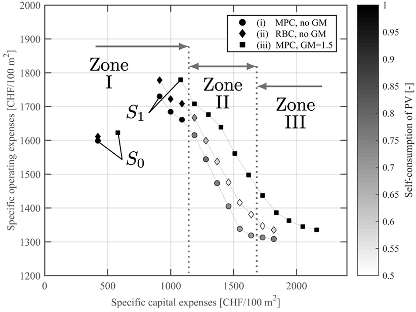
Figure 8. Pareto fronts for a single-family home when applying MPC (circles), RBC (diamonds), and MPC with a tight GM constraint (squares).

To understand the former behaviors, Figure 9 illustrates the evolution of both different cost contributions and the performance indicators with respect to the relaxation of ϵ-constraint of the respective fronts (i)–(iii):

• In the case of (i)–(ii), as presented in Figure 9A, a small solar thermal collector array is added to the initial system S₁ for the first solutions, thus leading to the slight decrease in operating costs (zone I). With the further increase in capital expenses, the unit is rapidly replaced by a photovoltaic array until reaching the maximal hosting capacity of the roof (zone II). Finally, in zone III, additional thermal and subsequently, electrical storage sizes are implemented to further improve the integration of the renewable energy system as expressed by both the rising self-sufficiency and self-consumption, however, solely merely enhancing the related economic benefit. Considering the applied costing parameters, the purely fossil fuel-based solution S₀ is the most economic configuration.

• In the case of (iii), as illustrated in Figure 9B, a considerable battery stack is installed a priori to the development of a photovoltaic array. The large difference in operating (or capital regarding comparison basis considered) expenses between the Pareto fronts (i and iii) can indeed be related to a non-efficient utilization of the different conversion devices and a stronger need of electrical storage capacity to decrease the building net power profile variance.

FIGURE 9

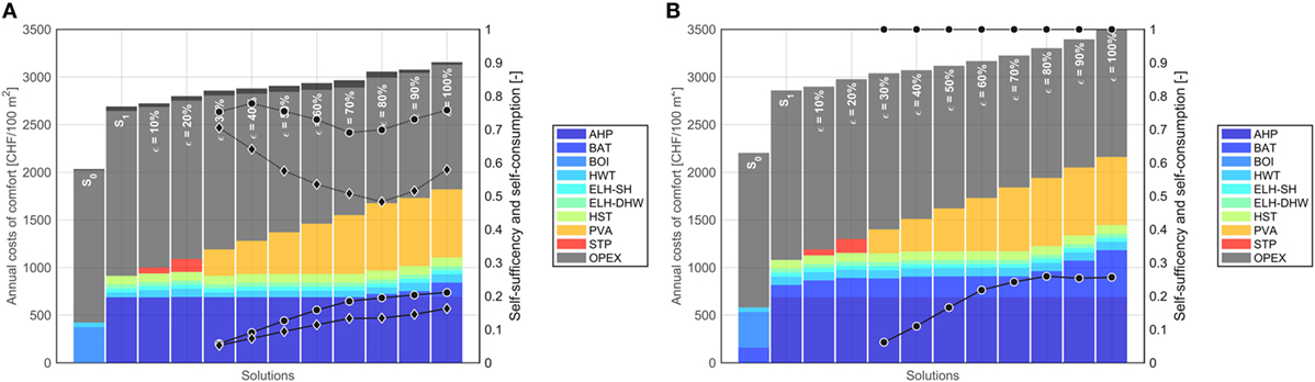
Figure 9. Multi-objective optimization results for a single-family house (Geneva, 1970–1980). Differences in operating costs between both control methods are represented by the dark gray stacked boxes. The self-consumption and self-sufficiency are represented through dotted and solid lines, respectively (MPC circles and RBC diamonds). (A) No ϵ_gm (i)–(ii). (B) ϵ_gm = 1.5 (iii).

To evaluate the influence of the dwelling size and affectation on the BES, Figure 10 presents the multi-objective optimization results performed for a large apartment block located in the Geneva-Cointrin climate region:

• In the case of (i)–(ii), Figure 10A depicts first a similar solution pattern as for the single-family house scenario, both in view of the BES design and the performance indicators. Nevertheless, a technology shift rapidly arises at a capital expenses value ϵ_inv = 0.4 and a combination of a solid oxide fuel cell (SOFC) CHP with an auxiliary natural gas boiler is implemented. This change triggers a strong increase in self-sufficiency in addition of a decrease in self-consumption; the latter behavior is related to the heat driven utilization of the CHP unit and the lack of electrical storage devices. Finally, for higher investment thresholds ϵ_inv = 0.8, a small air-source heat pump is installed to profit from the on-site generated power and thus engenders a rise in the self-consumption again.

• In the case of (iii), the main technology shifts already occur at lower capital expense thresholds as illustrated in Figure 10B. Indeed, for ϵ_inv = 0.2, an SOFC-CHP with an auxiliary natural gas boilers selected while the air-source heat pump is added at ϵ_inv = 0.5. Finally, starting from ϵ_inv = 0.9, a photovoltaic array is implemented, further increasing the system complexity. Similar to the single-family house scenario, a battery is required throughout the entire solution set to satisfy the ϵ_gm constraint; however, with the rise in BES complexity, the need for large electrical storage device strongly decreases.

FIGURE 10

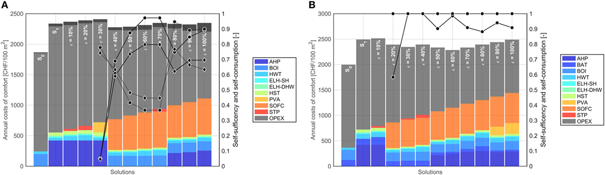
Figure 10. Multi-objective optimization results for an apartment block (Geneva, 1970–1980). Differences in operating costs between both control methods are represented by the dark gray stacked boxes. The self-consumption and self-sufficiency are represented through dotted and solid lines, respectively (MPC circles and RBC diamonds). (A) No ϵ_gm (i)–(ii). (B) ϵ_gm = 1.5 (iii).

3.1.1. Grid Impact

As presented in the section 2.3.3, an electrical storage equivalence (ESE) is applied to assess the load shifting potential of MPC when compared with RBC. Hence, Table 2 presents both the ESE exploited capacity C^ESE and round-trip efficiency ϵ^ESE in addition to the peak demand reduction $\mathrm{\Delta }{\dot{E}}_{\mathit{max}}$ for two different BES configurations (Figure 9). To compare the solutions generated with and without any ϵ_gm, a common operating costs basis is considered; both systems should reflect similar operating costs when operated without any ϵ_gm constraints. The resulting economic difference solely relies in the capital expenses and thus, translates as an additional investment from the building to achieve a grid-aware operation. Following observations can be stated from the presented results:

• (ϵ _inv = 0.3 and no ϵ_gm) The MPC is able to shift controllable loads during each typical day, the maximum exploited ESE capacity reaching 1.9 kWh/100 ⋅ m²; these changes in consumption are mainly related to an increase in the system efficiency (ϵ^ESE ≤ 0) since most of the on-site generated power is directly self-consumed. However, the optimal control approach has no influence on the peak demand, difference being positive or negative regarding the day considered.

• (ϵ _inv = 0.3 and ϵ _gm = 1.5) The used ESE capacity rises with the implementation of a strict ϵ_gm, the maximum values reaching 2.7 kWh/100 m². Nevertheless, the smoothing of the power profile engenders a higher electricity consumption for several days; indeed, the ϵ_gm has pushed the controller in decreasing the thermal conversion system efficiency by increasing the share of heat provided by electrical heaters over the heat pump. In regard to the definition in equation (6), the latter surge in power demand is required to satisfy the GM constraint without installing further storage equipment. Although the daily peak demands are drastically reduced for several days, it is important to note that the GM performance indicator does not guarantee the latter behavior (e.g., day 6).

• (ϵ _inv = 0.8 and no ϵ_gm) Given the higher on-site power generation from the large photovoltaic array, a consequent ESE capacity is noticed in this case, the maximum value being 7.0 kWh/100 m². However, the latter changes induce a higher consumption for several days since the produced electricity exceeds the current needs and thus, require use of storage.

• (ϵ _inv = 0.8 and ϵ _gm = 1.5) Similar to the previous investigation (ϵ_inv = 0.3), the exploited ESE capacity drastically rises while the related system efficiency drops with a tight ϵ_gm. Again, the operation with an ϵ_gm constraint does not ensure the decrease in peak demand.

TABLE 2

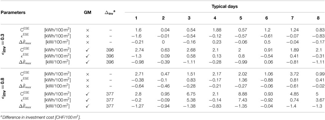
Table 2. Comparison of building energy systems (BES) solutions with and without GM constraint for a single-family house (Geneva, 1970–1980).

3.2. Multi-Building Level

Following the single-dwelling case studies, this subsection evaluates the benefit of MPC on the multi-building scale. By combining the building-specific optimization results in regard to the different topology parameters, a large solution space can be generated; the Pareto front is defined by selecting the solutions located on the space boundary of interest. A sub-urban commune located in Western Switzerland, comprising 629 registered buildings and around 6,800 inhabitants is first analyzed.

Hence, Figure 11 depicts two fronts couples regarding the considered electricity mix: 0.113 [kgCO₂-eq./kWhe] (bottom) and 0.376 [kgCO₂-eq./kWhe] (top). The first value reflects the actual situation, which mainly relies on hydro and nuclear energy sources (Prognos et al., 2016). However, since the hydro availability is rather low during strong demand periods (winter) while the national government is targeting a nuclear phase-out by 2050, a comparative mix value is applied additionally, assuming a homogeneous conversion from natural gas fired combined cycle plants. As observed, the original scenarios S₀ lies, as expected, on the left extreme of the aggregated Pareto fronts, thus representing the cost effective solution. With the increase in total comfort costs (i.e., total expenses), the environmental impact of the BES is strongly reduced (zone a) until reaching around 1,100 CHF/hab years after which, the slope significantly decreases (zones b and c). Interestingly, in the case of the carbon intensive electricity mix, an opposite evolution is observed; the slope increases beyond the latter cost threshold.

FIGURE 11

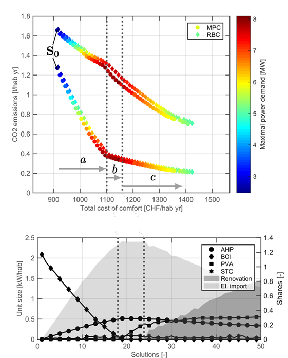
Figure 11. Pareto fronts for a sub-urban commune in Western Switzerland when applying MPC (circles) and RBC (diamonds).

To explain the latter behaviors, the lower graph in Figure 11 illustrates the evolutions of selected conversion units. Indeed, in the first phase (zone a), the purely fossil-based solutions (S₀) are gradually replaced by air-source heat pump based BES until completely removing all natural gas-powered boilers. This shift of energy carrier obviously engenders a strong impact on the power network which has to cope the related increase in both in peak demand (+208%) and energy consumption (+135%). In a second phase (zone b), photovoltaic arrays are rapidly installed to reduce electricity imports and thus the greenhouse gas emissions associated with the electricity mix. Finally, in the last phase (zone c), the building stock is gradually renovated, hence decreasing the required heat pump capacity as well as the peak power demand related to it (−35%). In addition, the photovoltaic array size is further increased until reaching the upper investment bound ϵ_inv = 1.

3.3. National Scope

Although being less useful to distribution network operators, an assessment on the national level provides interesting insights on the integration of renewable and distributed energy resources with respect to given system parameters. Indeed, the large-scale impact characterization represents an important tool for supporting public decision-makers within the context of strategic energy planning (Codina Gironès et al., 2015). Hence, similar to the single-commune case, Figure 12 illustrates the Pareto fronts for Switzerland, comprising 1.6 million registered buildings and around 8.1 million inhabitants. As observed, starting from the initial solution S₀, the CO₂ equivalent emissions rapidly decrease until reaching an inflection point at around 2,500 CHF/hab years. Similarly, an opposite behavior is observed in the case of carbon intensive electricity mix.

FIGURE 12

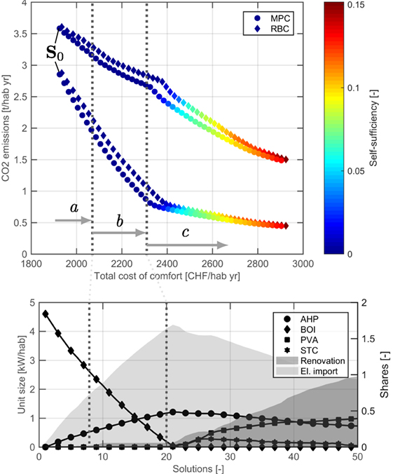
Figure 12. Pareto fronts for Switzerland when applying MPC (circles) and RBC (diamonds). The marker size reflects the renovation share of the current built environment.

From the lower graph of Figure 12, three transition steps are identified; similar to the previous multi-building investigation, in the first phase (zone a), the purely natural gas based solutions (S₀) are gradually replaced by air-source heat pump based BES. However, briefly after, a slight part of the national building stock is renovated, the latter share remaining relatively small until the complete phase-out of S₀ type configurations (zone b). After this point, both the share of renewable energy sources penetration and renovation are increasingly expanded until reaching the upper investment boundary ϵ_inv = 1 (zone c).

Finally, to assess the impact of MPC on the national scale, Table 3 presents performance indicators for three specific system solutions while Figure 13 displays the associated spatial integration of renewable energy sources (i.e., self-sufficiency). Similar to the single-building case studies, the use of MPC over RBC highly increases the share of self-consumption as well as self-sufficiency, values ranging from 0 to 19% and from 0 to 22%, respectively. From the economic perspective, the decrease in operating expenses varies between 1% for low investment solutions and 3% for more complex systems. It is worth noting that since the distributed power generation (E_gen) is solely performed using photovoltaic arrays, the latter remains identical for both control approaches.

TABLE 3

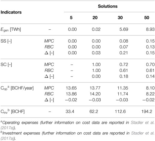
Table 3. National impact of MPC.

FIGURE 13

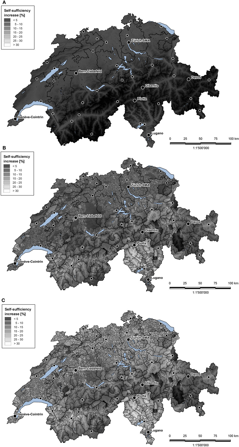
Figure 13. Increase in self-sufficiency in each commune with the rise in capital expenses. (A) Solution 20. (B) Solution 30. (C) Solution 50.

4. Conclusion

The presented work proposed a systematic method to simultaneously design and control optimal building energy systems with respect to the user interests. The former comprises a multidimensional data reduction process, the integration of a holistic technology structure and an ϵ-constraint multi-objective optimization approach to generated attractive solutions. In addition, through several modifications of the original problem formulation, the approach could be applied to assess the benefit of predictive control (MPC) in comparison with standard rule base control (RBC) techniques. The developed method has been demonstrated on the basis of several case studies, ranging from the single dwelling to the national scope using additional aggregation schemes.

Thus, the generated results suggested that the use of MPC for modern and complex BES represents a significant element in increasing the penetration of efficient and renewable-based energy systems within the built environment. Most notable observations can be summarized as follows:

• In regard to the considered boundary conditions, economically optimal BES designs are not including any renewable energy sources. However, the systematic generation of different complexer configurations nevertheless highlighted both the economic and environmental benefits engendered by the implementation of MPC. Results showed that the former strongly depend on the installed energy system, self-consumption differences varying between 0 and 27%.

• The design of gird-aware solutions through the implementation of an additional indicator, the grid multiple (GM), engenders a significant increase in investment costs while limiting the penetration of renewable resources at low investment thresholds. Nevertheless, the future integration of e-mobility might provide an interesting alternative to additional flexibility investments from the building side.

• In view of the assumptions on the boundary conditions, the preliminary assessment of the national potential of MPC suggests similar relative results as on the building level. While decreasing the operational energy bill, the use of predictive control strongly increases the share of self-consumption and self-sufficiency, differences ranging from 0 to 19% and from 0 to 22%, respectively.

In future, studies should investigate the impact of a multi-dwellings approach during the optimization process, hence assessing the potential of smart grids. The latter problem formulation enables the integration of grid-oriented operating constraints such as the maximal power flow values at the sub-station level which could not been implemented within the presented single-building method. In addition, a formal metric definition of flexibility should be investigated to properly assess the grid awareness of each system design.

Nomenclature

Subscripts
p	Period
t	Time
u	Units
build	Building
grid	Grid
Superscripts
+/−	Incoming/outgoing flow
′	Rule-based control index
dhw	Domestic hot water
max/min	Maximum/minimum
ng/el	Natural gas/electricity
sh	Space heating
Parameters
σ	Self-discharge rate [–]
d	Step duration [h] or [days]
$\dot{\text{E}}$	Uncontrollable electricity demand [kW]
f	Unit size bounds [kW] or [m2] or [m3]
inv	Investment cost function parameters [CHF] or [CHF/kW] or
	[CHF/kWh] or [CHF/m2] or [CHF/m3]
$\dot{\text{m}}$	Uncontrollable domestic hot water demand [kg/s]
op	Energy cost parameters [CHF/kWh]
Variables
$\dot{H}$	Chemical power flow [kW]
$\dot{R}$	Cascaded heat [kW]
$E∕\dot{E}$	Electrical energy [kW]/power flow [kWh]
F	Unit size [kW] or [kWh] or [m2] or [m3]
$m∕\dot{m}$	Water mass [kg]/mass flow [kg/s]
$Q∕\dot{Q}$	Thermal energy [kW]/power flow [kWh]
T	Temperature [K]
y	Unit activation (binary) [–]

Author Contributions

PS designed and implemented the methodology and model, acquired numerical data, produced the results, and wrote the article. LG contributed to the design of the model and methodology and acquired numerical data. He further revised the article and gave valuable hints for improvement of the content. AA reviewed the article and gave valuable hints for improvement of the structure and the content. FM contributed to the design of the methodology and gave valuable hints for the produced results.

Conflict of Interest Statement

The authors declare that the research was conducted in the absence of any commercial or financial relationships that could be construed as a potential conflict of interest.

Funding

This work has received support from the Swiss National Science Foundation under the NRP 70 Energy Turnaround Project (Integration of Intermittent Widespread Energy Sources in Distribution Networks: Storage and Demand Response, grant number 407040 15040/1) and the Swiss Centre for Competence in Energy Research on the Future Swiss Electrical Infrastructure (SCCER-FURIES) with the financial support of the Swiss Innovation Agency (Innosuisse–SCCER program).

Supplementary Material

The Supplementary Material for this article can be found online at https://www.frontiersin.org/articles/10.3389/fenrg.2018.00022/full#supplementary-material.

Abbreviations

AHP, air-source heat pump; BAT, battery; BES, building energy system; BOI, natural gas boiler; CDD, cooling degree days; CHP, combined heat and power; DRY, design reference year; DWT, domestic hot water tank; ELH, electrical heater; ESE, electrical storage equivalence; GHI, global horizontal irradiance; GM, grid multiple; HDD, heating degree days; HWT, hot water tank; LPEM, low temperature proton exchange membrane fuel cell; MILP, mixed-integer linear programming; MINLP, mixed-integer non-linear programming; MPC, model predictive control; PVA, photovoltaic array; RBC, rule-based control; SC, self-consumption; SOFC, solid oxide fuel cell; SS, self-sufficiency; STC, solar thermal collector; VAC, ventilation and air conditioning.

Footnote

1. ^Currently, several important building parameters (e.g., footprint area or floor number) are not required to be provided by law and thus are solely partly available in function of the good will of communes (smallest political entity in Switzerland).

References

Ashouri, A., Fux, S. S., Benz, M. J., and Guzzella, L. (2013). Optimal design and operation of building services using mixed-integer linear programming techniques. Energy 59, 365–376. doi: 10.1016/j.energy.2013.06.053

CrossRef Full Text | Google Scholar

Ashouri, A., Stadler, P., and Maréchal, F. (2015). “Day-ahead promised load as alternative to real-time pricing,” in IEEE International Conference on Smart Grid Communications (SmartGridComm) (Miami, FL: IEEE), 551–556.

Google Scholar

Bemporad, A., and Morari, M. (1999). Control of systems integrating logic, dynamics, and constraints. Automatica 35, 407–427. doi:10.1016/S0005-1098(98)00178-2

CrossRef Full Text | Google Scholar

Borel, L., and Favrat, D. (2010). Thermodynamics and Energy Systems Analysis: From Energy to Exergy. Lausanne: EPFL Press.

Google Scholar

Codina Gironès, V., Moret, S., Maréchal, F., and Favrat, D. (2015). Strategic energy planning for large-scale energy systems: a modelling framework to aid decision-making. Energy 90(Part 1), 173–186. doi:10.1016/j.energy.2015.06.008

CrossRef Full Text | Google Scholar

Collazos, A., Maréchal, F., and Gähler, C. (2009). Predictive optimal management method for the control of polygeneration systems. Comput. Chem. Eng. 33, 1584–1592. doi:10.1016/j.compchemeng.2009.05.009

CrossRef Full Text | Google Scholar

De Coninck, R., and Helsen, L. (2016). Practical implementation and evaluation of model predictive control for an office building in Brussels. Energy Build. 111, 290–298. doi:10.1016/j.enbuild.2015.11.014

CrossRef Full Text | Google Scholar

Domínguez-Muñoz, F., Cejudo-López, J. M., Carrillo-Andrés, A., and Gallardo-Salazar, M. (2011). Selection of typical demand days for CHP optimization. Energy Build. 43, 3036–3043. doi:10.1016/j.enbuild.2011.07.024

CrossRef Full Text | Google Scholar

European Environment Agency. (2012). Heating Degree Days – Trend in Heating Degree Days in the EU-27. Technical Report. Denmark: European Environment Agency. Available at: https://www.eea.europa.eu/data-and-maps/indicators/heating-degree-days-1 (Accessed: December 01, 2016).

Google Scholar

Fazlollahi, S., Bungener, S. L., Mandel, P., Becker, G., and Maréchal, F. (2014). Multi-objectives, multi-period optimization of district energy systems: I. Selection of typical operating periods. Comput. Chem. Eng. 65, 54–66. doi:10.1016/j.compchemeng.2014.03.005

CrossRef Full Text | Google Scholar

Fux, S. F., Benz, M. J., and Guzzella, L. (2013). Economic and environmental aspects of the component sizing for a stand-alone building energy system: a case study. Renew. Energy 55, 438–447. doi:10.1016/j.renene.2012.12.034

CrossRef Full Text | Google Scholar

Girardin, L., Marechal, F., Dubuis, M., Calame-Darbellay, N., and Favrat, D. (2010). EnerGis: a geographical information based system for the evaluation of integrated energy conversion systems in urban areas. Energy 35, 830–840. doi:10.1016/j.energy.2009.08.018

CrossRef Full Text | Google Scholar

Grossmann, I. E. (2012). Advances in mathematical programming models for enterprise-wide optimization. Comput. Chem. Eng. 47, 2–18. doi:10.1016/j.compchemeng.2012.06.038

CrossRef Full Text | Google Scholar

Kaufman, L., and Rousseeuw, P. J. (2009). Finding Groups in Data: An Introduction to Cluster Analysis. Hoboken, NJ: John Wiley & Sons.

Google Scholar

Lefèvre, M., Remund, J., Albuisson, M., and Wald, L. (2002). “Study of effective distances for interpolation schemes in meteorology,” in European Geophysical Society, 27th General Assembly (Nice, France: European Geophysical Society).

Google Scholar

Luthander, R., Widén, J., Nilsson, D., and Palm, J. (2015). Photovoltaic self-consumption in buildings: a review. Appl. Energy 142, 80–94. doi:10.1016/j.apenergy.2014.12.028

CrossRef Full Text | Google Scholar

Mavrotas, G. (2009). Effective implementation of the epsilon-constraint method in Multi-Objective Mathematical Programming problems. Appl. Math. Comput. 213, 455–465. doi:10.1016/j.amc.2009.03.037

CrossRef Full Text | Google Scholar

Oldewurtel, F., Ulbig, A., Morari, M., and Andersson, G. (2011). “Building control and storage management with dynamic tariffs for shaping demand response,” in 2nd IEEE PES International Conference and Exhibition on Innovative Smart Grid Technologies (Manchester, UK: IEEE), 1–8.

Google Scholar

Prognos, A. G., Infras, A. G., TEP Energy GmbH. (2016). Analyse des schweizerischen Energieverbrauchs 2000 – 2015 nach Verwendungszwecken. Technical Report. Bundesamt für Energie BFE. Available at: http://www.bfe. admin.ch/themen/00526/00541/00542/02167/index.html?lang=dedossier_id=02169 (Accessed: December 1, 2016).

Google Scholar

Rager, J. M. F. (2015). Urban Energy System Design from the Heat Perspective Using Mathematical Programming Including Thermal Storage. Ph.D. thesis, STI, Lausanne.

Google Scholar

Schütz, T., Schiffer, L., Harb, H., Fuchs, M., and Müller, D. (2017). Optimal design of energy conversion units and envelopes for residential building retrofits using a comprehensive MILP model. Appl. Energy 185(Part 1), 1–15. doi:10.1016/j.apenergy.2016.10.049

CrossRef Full Text | Google Scholar

Schütze, T., Schraven, M. H., Fuchs, M., and Müller, D. (2016). “Clustering algorithms for the selection of typical demand days for the optimal design of building energy systems,” in Proceedings of ECOS 2016 – 29th International Conference on Efficiency, Cost, Optimization, Simulation and Environmental Impact of Energy Systems (Solvenia).

Google Scholar

Section Bâtiments et logements. (2015). Registre fédéral des bâtiments et des logements – Catalogue des caractères Version 3.7. Technical Report. Neuchâtel: Office fédéral de la statistique (OFS). Available at: https://www.bfs.admin.ch/bfs/fr/home/registres/registre-batiments-logements.html (Accessed: December 1, 2016).

Google Scholar

Shepard, D. (1968). “A two-dimensional interpolation function for irregularly-spaced data,” in Proceedings of the 1968 23rd ACM National Conference, ACM ’68 (New York, NY: ACM), 517–524. Available at: http://doi.acm.org/10.1145/800186.810616

Google Scholar

SIA 2024. (2015). Données d’utilisation des locaux pour l’énergie et les installations du bâtiment. Technical Report. Zürich: Société suisse des ingénieurs et des architectes (SIA). Available at: http://www.webnorm.ch/collection%20des%20normes/architecte/sia%202024/f/2015/F/Product (Accessed: September 1, 2016).

Google Scholar

SIA 2028. (2008). Données climatiques pour la physique du bâtiment, l’énergie et les installations du bâtiment. Technical Report. Zürich: Société suisse des ingénieurs et des architectes (SIA). Available at: http://www.webnorm.ch/collection%20des%20normes/architecte/sia%202028/f/2010/F/Product (Accessed: September 1, 2016).

Google Scholar

Stadler, P., Girardin, L., Ashouri, A., and Marechal, F. (2017a). MILP Optimization of Building Energy Systems: Supplementary Information. Technical Report. Lausanne, Switzerland: EPFL.

Google Scholar

Stadler, P., Girardin, L., and Maréchal, F. (2017b). “The Swiss potential of model predictive control for building energy systems,” in 7th IEEE PES International Conference and Exhibition on Innovative Smart Grid Technologies, Europe (Turino, Italy).

Google Scholar

Statistical Office of the European Communities. (2015). Energy Balance Sheets: 2013 Data. Technical Report. Luxembourg: Eurostat. Available at: http://ec.europa.eu/eurostat/web/energy/data/energy-balances (Accessed: September 1, 2016).

Google Scholar

Wakui, T., and Yokoyama, R. (2015). Optimal structural design of residential cogeneration systems with battery based on improved solution method for mixed-integer linear programming. Energy 84(Suppl. C), 106–120. doi:10.1016/j.energy.2015.02.056

CrossRef Full Text | Google Scholar

Weber, C., Maréchal, F., Favrat, D., and Kraines, S. (2006). Optimization of an SOFC-based decentralized polygeneration system for providing energy services in an office-building in Tokyo. Appl. Therm. Eng. 26, 1409–1419. doi:10.1016/j.applthermaleng.2005.05.031

CrossRef Full Text | Google Scholar

Zhao, Y., Lu, Y., Yan, C., and Wang, S. (2015). MPC-based optimal scheduling of grid-connected low energy buildings with thermal energy storages. Energy Build. 86, 415–426. doi:10.1016/j.enbuild.2014.10.019

CrossRef Full Text | Google Scholar