A Simple Approach to Modeling Rural and Urban District Heating

GRAPHICAL ABSTRACT

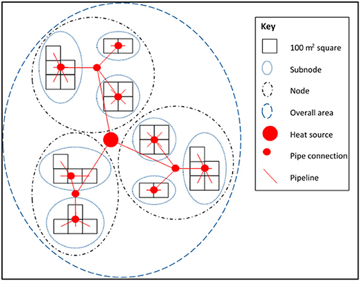
Graphical Abstract. An example of the node, subnode structure used in the model.

Introduction

The EU aims to, by 2020, reduce CO₂ emissions to 20% of the 1990 levels (European Parliament, 2012). Compared to the UK 1990 emission levels of 794.2 MtCO₂e, current UK emissions have been decreasing, down to 467.9 MtCO₂e in 2016; however further work must be done to meet the EU targets (BEIS, 2018). In order to meet the EU targets, emissions related to the heating of buildings need to be reduced to almost zero [Department of Energy and Climate Change (DECC), 2013]. Reducing building heating emissions to near zero would be best achieved through electrifying heating or decarbonizing the heat supply. Electrifying heating is likely to increase the strain on the national grid beyond its current maximum capacity, requiring extensive and expensive restructuring (Wilson et al., 2013). Decarbonizing the heat supply could be achieved by switching building heating from natural gas to district heating.

District heating is a method of providing thermal energy to a number of customers from a centralized heat source (or sources) through the pumping of a heat transfer fluid around a pipe network. District heating is based around a network comprised of: thermal energy generating unit(s), the pipe network, and customer substations (Frederiksen and Werner, 2013). District heating can act as a flexible and secure source of heat that can use local and environmental energy sources, which would not be utilized otherwise. Energy sources include: waste heat from industry, waste incineration, combined heat and power and renewables (Sipilä, 2011). The level of decarbonization achieved by district heating is highly dependent on the heat supply used; the best levels of decarbonization occur if the fuel used is green or carbon neutral. Despite the decarbonization benefits and due to the high costs of network installation, particularly in rural areas, district heating may not be economically viable in every case. A model that could be used to assess the economic and environmental feasibility of any new network that could be implemented quickly and easily by a non-technical staff member at a local authority would be useful. The creation of such a model would allow local authorities to assess the feasibility of more potential networks, increasing the uptake of district heating.

This paper explores the initial stages of such a model, focusing on modeling the hourly variation in the local area heat demand, using Darley Dale in Derbyshire, UK as a case study. Darley Dale has a population of 5,400 (ONS, 2014) and a yearly heat demand of 50,000 MWh (BEIS, 2018). Darley Dale, alongside an urban town and an urban city is used to highlight the differences in modeling heat demands in areas of different population densities to see if the same modeling process can be used for all varieties of population density. Monte Carlo simulations are used to assess the assumptions necessitated by the simple nature of the heat demand model, investigating if the initially proposed methodology is adequate for use. HJ Enthoven, a lead acid battery recycling plant, provides primary data for the paper. HJ Enthoven only operate an industrial site and not a district heating network and were unable to provide primary district heating network data.

Rural District Heating

In the UK, a rural area is classified as an area with a population of fewer than 10,000 people (ONS, 2011a). Due to the low population, rural areas tend to have both lower population densities and lower heat demand densities; therefore rural district heating networks have low revenues compared to the network installation costs (Nilsson et al., 2008). The government has defined the annual heat demand density needed for district heating to be profitable as 26,000 MWh/km² [Department of Energy and Climate Change (DECC), 2009]. The UK CHP development map shows that large proportions of the rural areas of the UK have annual heat demand densities of < 20,000 MWh/km² (BEIS, 2018), less than the threshold for profitable district heating. However, district heating can still be viable in areas of low heat demand density, particularly in locations with an already existing heat supply (Frederiksen and Werner, 2013).

The potential for new rural district heating networks should even be considered in countries, such as Sweden, where the urban heat market is almost saturated with district heating. Rural district heating has only been implemented to a large extent in Iceland and Denmark (Reidhav and Werner, 2008); however, even in Iceland and Denmark, rural district heating is not very common (Nilsson et al., 2008). In the UK, roughly 9 million people or 17% of the population, live in rural areas [(Department for Communities and Local Government (DCLG), 2014)] meaning that the annual rural domestic heat market is ~0.3 PJ/yr (BEIS, 2017a,b). From the UK CHP development map, urban areas typically have annual heat loads of 10,000–200,000 MWh/km² whereas rural areas tend to have heat loads < 10,000 MWh/km² (BEIS, 2018).

District Heating Modeling

Many types of district heating models exist, with a differing range of goals and uses. Selecting the model most suitable for use in a particular case and application requires a thorough understanding of the range of models that exist, along with each models' uses and limitations. District heating models can consider anything from the entire network structure to an individual customer. In this paper only models of entire district heating networks will be considered.

District heating models can be either statistical or physical. Statistical models are time series or neural network based, are easy to build and understand but require primary measurements for validation (Wojdyga, 2014). The requirement of primary network data make statistical models unsuitable for use, due to the lack of primary data provided from industry.

Physical models consider the entire structure of a district heating network, which makes them easy to modify but complex and computationally intensive. Instead of primary measurement validation, physical models only require simple network data inputs such as the network topology, pipe and insulation specifications and the pump characteristics (Larsen et al., 2002; Wang et al., 2016).

Physical models need to be simplified to reduce the computing power required, simplification is achieved through the node method, otherwise called the process of aggregation. The node method substitutes the existing loop and tree structure of a network with lines and short branches, reducing the network complexity and computational intensity. The simplified models are generated using steady state flow conditions. During aggregation, important physical properties such as water volumes, time delays and mass flows are preserved (Palsson et al., 1999; Jie et al., 2012). Aggregation can be achieved using one of two techniques: the German or the Danish methods. The German and the Danish methods enable the network complexity to be reduced from 44 pipes to 10 or 3, respectively. Both methods preserve all physical parameters bar: the heat losses for the German method and the pressure distribution for the Danish method (Larsen et al., 2004). The node method does not maintain an entire network structure, which would make network modifications difficult, therefore the node method is unsuitable for use.

Another method that can be used to simplify district heating networks is studying the relevant influences that the differing factors have on the overall heat demand. Studying the factors identifies influential factors that must be conserved and insignificant factors that can be omitted. The most influential factors on the heat demand are the outdoor temperature and the customer behavior (Dotzauer, 2002); therefore district heating models exist that only consider the outdoor temperature and customer behavior. As insignificant factors have been omitted, temperature, and behavior models can have as few as four to seven design equations, making them simple and requiring only small amounts of computational power to operate (Werner, 1984; Dotzauer, 2002). Other researchers have suggested that temperature and behavior models are oversimplified which will introduce error into the work (Heller, 2000) as the temperature component itself must be split into four different factors (Heller, 2002). Due to the possible oversimplification and consequent errors, splitting the overall heat demand into components is unsuitable for use.

Short term heat demand can be modeled deterministically or predictively using time series. Deterministic models use complex simulations to predict the physical behavior of the buildings in the study. The complex deterministic simulations require simulation software as shown in Table 1.

TABLE 1

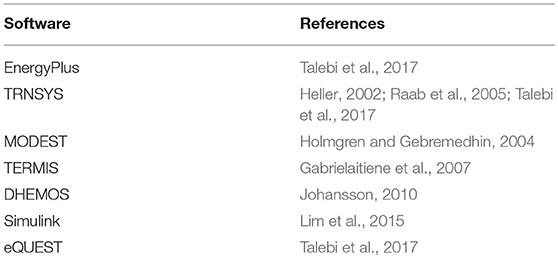
Table 1. Simulation software used in the modeling of district heating.

Deterministic models generate accurate results but require extensive data inputs and have high computational costs. The non-technical staff member who this paper is aimed at is unlikely to have access or be able to operate engineering specific software, therefore deterministic modeling is unsuitable for use.

Predictive models use equations to fit curves to the demand profiles (Talebi et al., 2016). Predictive modeling can be achieved using ARMA models, Kalman filters or artificial intelligence models. ARMA models smooth expected real world data to that of a predicted demand (Amjady, 2001). Kalman filters estimate the value of the next time step based on the value being experienced currently. For each estimation, the current difference between the expected and real value is used to determine which one of several filters will be chosen (Palsson, 1993; Talebi et al., 2016). Artificial intelligence models cover a range of options: artificial neural networks (ANN), fuzzy neural networks (FNN), and support vector machines (SVM) (Talebi et al., 2016). ANN are the only examples of the machines that consider social parameters and consequently can have the highest levels of accuracy (Zhang et al., 1998). ANN require validation through real network data, allowing the model to train and develop, thereby improving the model accuracy (Keçebaş et al., 2012). ANN can over-fit the problem as well as having large data requirements. Some research suggests that SVM give the best results (Park et al., 2010), but SVM are limited in practical use by the data required; which must be highly precise (Chen et al., 2004). All of the predictive options are computationally intensive and highly specific, making the modeling type too complex for a non-technical individual to use and making predictive modeling unsuitable for use.

It is possible to model a district heating network using historical data, where the district heating model is validated using the historical operating records of an existing network (Noussan et al., 2014). Once validated, the model is used to predict future network performance using the predicted temperature and weather. Historical models use a concept called a heating degree day which is the difference between the outdoor temperature and a reference temperature, at which point a buildings heating system is turned on (Raine et al., 2014; Raine, 2016). The heat demand of a building is directly proportional to the heating degree day (Pirouti, 2013; Talebi et al., 2016). In the UK, the reference temperature is usually set as 15.5°C (Carbon Trust, 2012). Historical degree day values can be accessed for a time period of several years (Met Office, 2015), although weather conditions can vary significantly year to year requiring heating degree day models to be validated for future performances (Noussan et al., 2017). Due to readily available degree day records, the heating degree day method is suitable for use.

Another historical modeling type uses customer meter readings to model a district heating network. Meter reading modeling types use the water temperature, flow rate or gas bills to model the overall network heat demand (Wang et al., 2013; Fang and Lahdelma, 2014; Spoladore et al., 2016). The results of customer meter reading studies vary significantly when the customer heating system changes from being electrical to hydronic, making customer meter reading modeling inaccurate in areas with a large building heterogeneity (Kipping and Trømborg, 2017). Due to the small time step and the large number of buildings in the studies, customer meter reading models are data and computationally intensive (Talebi et al., 2016). The data and computational intensity makes customer meter reading modeling unsuitable for use.

To reduce the number of buildings being individually modeled in the work and consequently reduce the complexity of the model, a district heating network can be modeled using the archetype building method. The archetype method works by grouping all buildings into a series of categories and representing each category with an archetype building. The accuracy of archetype modeling is heavily dependent on the number of archetype categories used and the accuracy of each individual archetype model. Individual archetype models are regression based, finding a typical demand profile for that building category (Talebi et al., 2016). Examples of archetype models have been run across a range of public buildings, including schools finding that around 50% of buildings in each category show similar results to that of the archetype building (Gaitani et al., 2010; Lara et al., 2015). The low data and computational needs of the archetype building method makes it suitable for use.

Current district heating models have limitations, which impact district heating implementation (Talebi et al., 2016). A heterogeneous building stock is difficult to accurately model using a single modeling type. Many models only estimate the total yearly energy demand instead of an hourly, or more accurate demand profile. The size of the heat source or the network costs can be determined using estimations of yearly energy demand however, determining the hourly supply and demand requires a different strategy. Many of the models when used in practice, have errors of up to 20%, with extreme cases having errors up to 60% (Nouvel et al., 2013; Fonseca and Schlueter, 2015). Finally, many of the models are highly data intensive, affecting cost and applicability. The research into district heating modeling shows the importance of creating a model that can work on a heterogeneous building stock and can estimate an hourly demand profile with low errors and low data intensity.

Methodology

The overall aim of this paper was to produce a heat demand model that was simple enough for a non-technical individual to use. The model quantified the hourly variation in the local area heat demand using a node structure that was easy to modify. The model was built using the heating degree day and archetype building methods.

The initial stage of the modeling work was to follow a geographical information systems (GIS) technique to build an energy map of the area. The energy map looked at both commercial and domestic buildings and identified the areas of high heat demand density and customers with a large heat demand. The commercial energy mapping was based on a technique used by Parsons Brinckerhoff (Parsons Brinckerhoff, 2011), using CIBSE energy benchmarks TM46 [Chartered Institution of Building Services, Engineers (CIBSE), 2008], the Energy Information Administration (EIA) commercial buildings energy consumption study (EIA, 2016), Google Maps, and Google Street View. The CIBSE energy benchmarks TM46 gave the annual energy use of archetype buildings in kWh/m². The EIA energy consumption study split the typical energy use of archetype buildings into individual uses. CIBSE and EIA studies combined were used to give the annual thermal energy use for heating in kWh/m² of archetype building categories. Google Maps and Google Street View were used to identify every possible heat user in the local area alongside the location, use and total measured floor area. The use of Google Maps introduced error; the error was acceptable as the energy maps only estimated and did not quantify the energy demand. Domestic energy mapping was carried out though converting population density into energy density (Finney et al., 2012; BEIS, 2016). The domestic energy mapping required assumptions of an average of 2.37 people per dwelling, that the average UK domestic heat usage is 20.5 MWh per home per annum (Finney et al., 2012) and that the 2011 UK census data was still accurate (ONS, 2011b).

The energy maps were used to give an estimation of the yearly heat demand in the local area but did not model the heat demand on an hourly basis and were not accurate. The hourly heat demand modeling was done based on an industrial, archetype building model, which was centered around heat demand curves generated Arup (Arup, 2007). The industrial model used the heating degree day and archetype building methods and produced hourly heat demand curves for seven archetype building types. The heat demand curves showed how the hourly thermal load per unit area of a buildings total floor space (kW/m²) changed over a day. For each building type twelve curves were generated, each one representing a typical day of heat demand variation for each of the 12 months. The industrial model grouped every building into one of the following categories: retail, commercial, food and drink, hotels, residential, non-residential institutions and assembly and leisure. The monthly degree day values were determined using daily temperature data from a local weather station throughout the course of each year, as shown in Equations (1, 2):

$T_{dd}=\frac{{\displaystyle {\sum }_{t=0}^{t_{max}}{x}_t}}{t_{max}}(1)$

Where

$x_t=\{\begin{array}{c}{T}_{ref,t}-T_t,if{T}_{ref,t}>T_t\\ 0,if{T}_{ref,t}<T_t\end{array}(2)$

The monthly degree day value (T_dd) (°C/h) was based on the sum of the hourly differences between the reference temperature (T_{ref, t}) (°C) and the external temperature (T_t) (°C), provided the reference temperature was greater than the external temperature, divided by the number of hours in the month (t_max) (hour). The monthly degree day values were used to make monthly temperature dependent factors (TDF), as shown in Equation (3).

$\begin{array}{r}\text{TDF}=\frac{T_{dd}}{T_{dd(max)}}\end{array}(3)$

The monthly TDF was the ratio between the monthly degree day value and the maximum monthly degree day value (T_{dd (max)}) (°C/h).

The industrial model gave curves of hourly heat demand per unit area of total floor space for each archetype building type for each of the 12 months. The aim of this paper was to generate curves of hourly thermal load, representing every building within a set area, for each of the four heating seasons. As a result, significant adaption had to be made to the industrial method. The 12 monthly curves were averaged into four heating season curves. The four seasons ran from 20th March to 20th June, 21st June to 21st September, 22nd September to 21st December and 22nd December to 19th March. The curves of hourly thermal load for each building type were calculated as shown in Equation (4).

$\begin{array}{r}Q=Q_{Area}A\end{array}(4)$

The hourly heat demand (Q) (MW) was a function of the hourly heat demand per building area (Q_Area) (MW/m²) and the total building floor area (A) (m²). The individual archetype building heat demands were compiled to make a total hourly building heat demand within a set area as shown in Equation (5).

$\begin{array}{r}{Q}_{Square}={\sum }_{i=1}^N{Q}_i\end{array}(5)$

The total hourly building heat demand within a square of 100 m² (Q_Square) (MW) was a sum of all of the individual hourly building heat demands (Q_i) (MW) for the N buildings within that area.

The paper calculated the total hourly building heat demand within a modeled area. The modeled area was split into a node, subnode structure. The structure was based around a heat source, splitting the modeled area into nodes, then subnodes and finally squares of 100 m² size, as shown in Graphical Abstract. The pipelines connecting the nodes to heat source were assumed to travel in the shortest possible straight line distance from the heat source to the center of each square of 100 m² via the center of the node and subnode. An assumption was made that no distance of pipe is needed to connect the buildings located inside the squares of 100 m² to the pipe connection at the center of the square.

For each square, the total number of buildings in each archetype building category was counted and used to calculate the total floor area of that building category as shown in Equation (6). Equation (6) was based on an assumed area for each building type in the study.

$\begin{array}{r}A=A_{A,Tot}={A_{A,Assumed}N}_A\end{array}(6)$

The total area of building category A (A_{A, Tot}) (m²) was proportional to the assumed area of buildings of that category (A_{A, Assumed}) (m²) and the number of buildings of that category (N_A).

In rural areas the distances between the heat source and customers could be over 1 km (Finney et al., 2011). The large distances meant that the model must consider the time delays and heat losses that occurred in the pipes. Time delays were based on an assumption of 2 m/s water velocity (Olsen, 2014). The time taken for the heat demand of a square to meet the heat source was dependent on the velocity in the pipes and the pipe length as shown in Equation (7).

$\begin{array}{r}t=\frac{L}{v}\end{array}(7)$

The time taken for the water to travel down a pipe (t) (s) was proportional to the pipe length (L) (m) divided by the water velocity (v) (m/s).

Heat losses were calculated per meter of pipe length, as shown in Equation (8).

$\begin{array}{r}{Q}_L=\frac{2\pi kL(T_i-T_o)}{ln(\frac{D_o}{D_i})}\end{array}(8)$

The heat loss (Q_L) (MW) was proportional to the thermal conductivity (k) (W/m.°C), pipe length and temperature difference across the pipe walls (T_i – T_o) (°C). Heat loss was inversely proportional to the natural log of the outer pipe diameter (D_o) (m) over the inner pipe diameter (D_i) (m).

The heat demands experienced in the center of each subnode, node and at the heat source were calculated, as shown in Equations (9–11).

$\begin{array}{r}{Q}_{Subnode,n}={\sum }_{i=1}^N{Q}_{Square,i}{Q}_{l,i}\end{array}(9)$

$\begin{array}{r}{Q}_{Node,n}={\sum }_{i=1}^N{Q}_{Subnode,i}{Q}_{l,i}\end{array}(10)$

$\begin{array}{r}{Q}_{Source}={\sum }_{i=1}^N{Q}_{Node,i}{Q}_{l,i}\end{array}(11)$

The heat demand experienced in the center of each subnode, node or the heat source (Q_Subnode, Q_Node) (MW) was a sum of all the heat demands of the components (Q_Square, Q_Subnode, or Q_Node) (MW) and the heat losses experienced in the pipes (Q_l) (MW) for the N components within that area. Where n represents the possibly different “Subnodes” or “Nodes.”

The model generates hourly curves of the heat demand experienced by the heat source for each of the seasons. The model was simple to understand, did not require large amounts of computing power and was quick to run. The node, subnode structure enabled easy modification through the addition or removal of nodes, subnodes, or squares. An example of a modification of the model is through a maximum allowable heat loss in each pipe. A maximum allowable heat loss as a percentage of the total heat demand in each pipe could be set. Any pipe that exceeded the maximum allowable heat loss was deleted. Deleting pipes instantly removed any nodes, subnodes or squares with heat losses that exceeded the set value and were unsuitable for use in the district heating network.

A disadvantage of the model was the number of assumptions used, including: that each building in a category was of the same set size, each building in a category had a heat demand curve as described by the industrial model and each pipe length traveled in the straight line distance from the customer to the heat source via the center of the subnode and node. The effect of the inaccuracies on the results was assessed using Monte Carlo simulations in the Goldsim software package (Goldsim, 2011).

Comparing Rural to Urban District Heating Networks

One of primary the goals of the paper was to investigate if the same generic modeling process could be used in areas of different population densities, such as rural and urban or towns and cities or if the model would need modification from population density to population density. To investigate the effects of the different population densities, three case studies were modeled: a rural location, a heavily populated urban location and a sparsely populated urban location. As the comparison was between areas of different population densities, not different areas in the world the same weather data was used for all three. The weather data came from a weather station in the Derbyshire Dales, located at 53°15′41.0″N 1°44′03.5″W (Met Office, 2015).

Case Study 1 (Rural Location)—Darley Dale, England

The first case study was based around HJ Enthoven, a lead-acid battery recycling plant located in Darley Dale, England. HJ Enthoven is the largest producer of recycled lead in Europe, producing 80,000 tons of lead and propylene annually from over 150,000 tons of lead-acid batteries (ECOBAT, 2017). HJ Enthoven is based near the towns of Darley Dale (population 5,400), Matlock (9,400), Rowsley (500), Bakewell (4,000), Youlgreave (1,000), and Cromford (1,400) (ONS, 2014). The Darley Dale case study was used as an example of a rural area with a small population density where the heat source is located outside of the rural township.

Case Study 2 (Heavily Populated Urban Location)—Sheffield, England

The second case study was based around Veolia Sheffield, a municipal solid waste incineration plant. The plant is capable of producing up to 19 MW of electricity and 60 MW of heat, combusting 225,000 tons of waste per annum (Veolia, 2014). Sheffield is the fifth biggest city in the UK with a population of 530,000 (ONS, 2009). The Sheffield case study was used as an example of a heavily populated urban area.

Case Study 3 (Sparsely Populated Urban Location)—Hayange, France

The third case study was based around a British Steel plant located in Hayange, France. The plant manufactures steel rail sections, special profiles, and wire rod, employing over 400 people (British Steel, 2017). Hayange is a town in France with a population of 15,000 (Hayange, 2017). The Hayange case study was used as an example of a sparsely populated urban area.

Results

The model was run for the three case study areas, generating hourly curves of heat demand for each of the four heating seasons, as shown in Figure 1. The maximum allowable heat loss in the first case study was set at 40% to match the local heat supply. The maximum allowable heat losses in the other two case studies were set to ensure that all of the three case studies had as close as possible to the same maximum hourly heat demand. Controlling the maximum hourly heat demand through maximum allowable heat losses is unavoidably imprecise, meaning that case study 2 has a higher peak heat demand than case studies 1 and 3. The lack of precision is acceptable as the paper is more interested in the shapes of the curves produced than the peak heat demands.

FIGURE 1

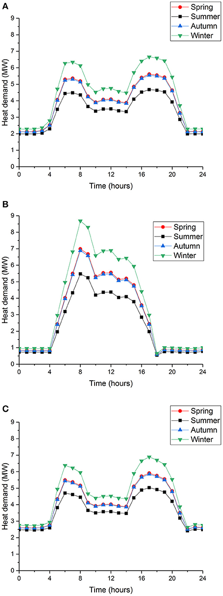
Figure 1. (A) The hourly heat demand profiles generated using case study 1, Darley Dale, England, with a maximum allowable heat loss in the pipes of 40%. (B) The hourly heat demand profiles generated using case study 2, Sheffield, England, with a maximum allowable heat loss in the pipes of 7%. (C) The hourly heat demand profiles generated using case study 3, Hayange, France, with a maximum allowable heat loss in the pipes of 45%.

Figure 1 shows the heat demand profiles of the three different case studies, showing the differently shaped curves generated using the same modeling technique. The differently shaped curves are because the different case studies have a different spread of building types. Figures 1A,C represent the rural case study (case study 1) and the urban case study with a small population density (case study 3). Both of the figures show maxima in the morning and evening, and minima in the middle of the day and at night. The position of the maxima and minima show that the buildings in case studies 1 and 3 are occupied during the morning and the evening, similar to the occupation characteristics of domestic buildings. Figures 1A,C prove that case studies 1 and 3 are comprised of a large number of domestic buildings; as shown in Table 2. Case studies 1 and 3 have high heat losses in the pipes, 40 and 45%, respectively, which is due to the long pipe lengths connecting areas of small heat demand. A district heating network with a large proportion of domestic customers would require a different investment type when compared to a network with more commercial customers. Domestic customers require as much and sometimes more support and information than commercial customers, generating less profit per unit sale (Lygnerud and Peltola-Ojala, 2010). A district heating network with a high proportion of domestic customers would struggle to make a viable business case.

TABLE 2

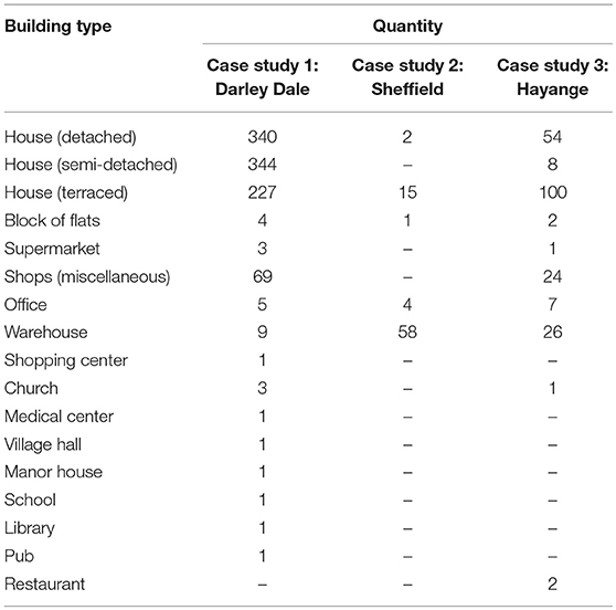
Table 2. Buildings used in each case study model.

As the aim of paper was investigate if the same modeling technique could be used in different areas of population density, all buildings in the case study areas were included, even domestic buildings. Figures 1A,C prove that, when following this modeling process, large numbers of domestic customers were included for areas of small population density. The modeling technique, particularly the stage where the buildings in each area of 100 m² were counted, will need to be modified to ensure that only larger domestic buildings, such as a block of flats, are included. Blocks of flats, as well as housing associations, are often regarded as anchor loads for a new district heating network (Hawkey, 2009).

Anchor loads are heat customers with large, stable and constant heat demands that are key to a network's success (Hawkey et al., 2013). The development of a district heating network often begins by identifying anchor loads to guarantee the infrastructure costs of the network can be covered through heat sales (Davies and Woods, 2009; Hawkey, 2009). Anchor loads help to reassure investors that may consider district heating to be a risky investment [Department of Energy and Climate Change (DECC), 2009].

Figure 1B represents the urban area with a large population density (case study 2). The figure has a maxima in the middle of the day and a minima for the rest of the time. The positions of the maxima and minima in case study 2 are similar to the occupation profiles produced by commercial properties, proving that case study 2 is largely comprised of commercial buildings; as shown in Table 2. Case study 2 has low heat losses, 7%, as the network has short pipe lengths that connect squares of large heat demand.

Table 2 shows that the case study with the large population density (case study 2) is comprised of a small number of large commercial buildings, which can act as anchor loads. The case studies with the smaller population densities (case studies 1 and 3) are comprised of many small domestic buildings. Urban areas with large population densities tend to have many large commercial buildings that are located near to possible heat sources. Areas with smaller population densities tend to have fewer large commercial buildings that are more dispersed. Figure 2 shows the geographical spreads of the three case studies, showing the location of the heat sources and the customers. The maps in Figure 2 are generated using QGIS software.

FIGURE 2

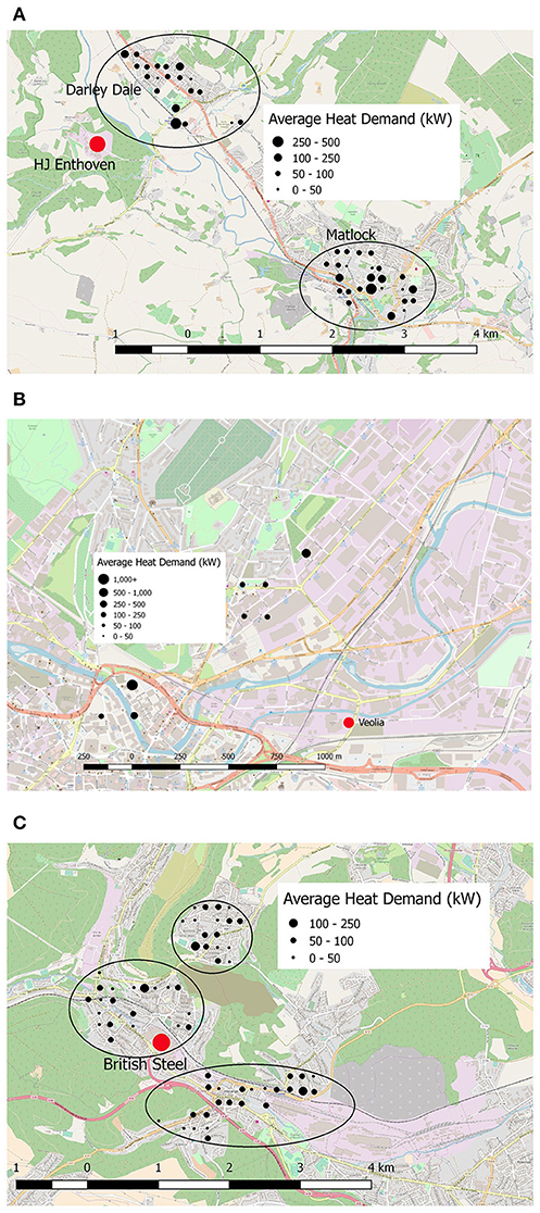
Figure 2. The size and locations of the heat source (in red) and customers (in black), showing the clusters of heat customers (in black rings) in each case study area. (A) GIS map showing the heat source and customers in case study 1: Darley, England. (B) GIS map showing the heat source and customers in case study 2: Sheffield, England. (C) GIS map showing the heat source and customers in case study 3: Hayange, France (Geofabrik, 2017).

Figure 2B shows that the customers in the densely populated case study (case study 2) are located close to the heat source. Case study 2 has a scale four times smaller than in case studies 1 or 3; as shown in Figures 2A,C. Figure 2B shows that possible heat customers can be located in any direction from the heat source in an area of large population density. Figures 2A,C show that the possible heat customers in the sparsely populated case studies (case studies 1 and 3) can only be located in clusters, in the built-up land surrounded by areas of green space.

The case studies with smaller population densities (case studies 1 and 3), have total pipe lengths of 22.0 and 32.8 km, respectively. The case study with the larger population density (case study 2), has a significantly smaller pipe length of 5.4 km. The rough differences in pipe length between more and less densely populated areas is by a factor of 4–6. As the capital costs of the pipe lengths and the heat losses are both proportional to pipe length (Raine, 2016), the capital costs of the pipe length and heat losses are roughly 4–6 times smaller for a network in an area with a large population density. The difference in costs is likely to become significant when the techno-economic modeling is applied. Potentially, the difference in pipe lengths will require different business cases or series of financial incentives to be applied in areas of differing population density.

The three case studies varied significantly in the number, and locations of the customers as well as heat losses in the pipes. The less densely populated case studies have hundreds of individual customers on the network, with at least 70% of the customers coming from domestic sources. The customers were shown to be clustered in the built up land surrounded by areas of green space. The heat losses in the less densely populated case studies were shown to be 40 and 45% of the overall heat demand. In comparison, the more densely populated case study was shown to have less than a hundred individual customers, with < 25% of the customers being from domestic sources. The customers were shown to have a greater dispersion around the heat source. The heat losses in the more densely populated case study were shown to be 7% of the overall heat demand. It was shown that the less densely populated case studies have pipe lengths 4–6 times longer than the more densely populated case studies. The overall heat demand of the network is dependent on the number, type and location of the customers and the heat losses in the pipe.

Model Validation

A primary goal of this paper was to keep the methodology simple enough to allow a non-technical individual to use, meaning several assumptions were made. The assumptions introduce the possibility of inaccuracy into the model, the extent of which was assessed both internally and externally. The internal assessment was completed using Monte Carlo simulations. Normally, the external assessment would be completed using primary district heating network data or a similar model. No existing district heating networks provided primary data for use in this study and due to novel nature of the work, external models that could be used as a comparison do not exist. Using an existing model would require more assumptions to be made than are already in the work, the accuracy of which would need assessing. Instead, the external validation comes from the industry confidence in the industrial model; the industrial model is generated based on industry experience (Arup, 2017). The external validation is sufficient for industry and is therefore the approach used in this work as it ties the data back to genuine field data.

Monte Carlo simulations were used to assess the accuracy of the key assumptions. Monte Carlo simulations re-ran the model thousands of times, varying the inputs, and measuring the variation in the model output. The assumptions that were assessed are: (1) the assumption that each building in the same archetype category is of a standard assumed size, (2) the assumption that each building in the same archetype category has the same hourly heat demand profile as described by industry and (3) the assumption that the pipe route runs in the shortest possible straight line distance from the heat source to the customer via the center of the nodes and the subnodes.

It is expected that on a network wide scale the inaccuracies from the assumptions will not be significant due to the large sample size, meaning that the average will not be significantly affected. In cases with large variance in the input data however, the average is likely to be significantly affected, meaning that the inaccuracies from the assumptions will be significant. The data used to validate the assumptions came from a series of studies into building size and heat demand variation [Burzynski et al., 2011; Building Research Association of New Zealand (BRANZ), 2014; Balcombe et al., 2015; BRE Trust, 2015; EIA, 2016; Törnros et al., 2016] and from comparing the length of an existing district heating network to the shortest possible straight line route (Finney et al., 2011). Studies from outside of the UK were used to increase the sample size and therefore the Monte Carlo accuracy. In order to account for the variation in building types from country to country, the data sets were normalized to themselves before being compared against each other. Using data from countries outside of the UK allowed the model to be assessed immediately, despite the lack of UK specific data. As UK studies are found investigating building heat demand and size variation, the Monte Carlo work can be updated.

The probability distributions that were loaded into Goldsim are based off the distributions found studying the variation in building sizes, heat demands and networks lengths. The distributions were as follows. For the building size assumption (1): a normal distribution with a mean of 1 and a standard deviation of 1.96. For the building heat demand assumption (2): a normal distribution with a mean of 1 and a standard deviation of 0.212. For the network route variation assumption (3): a pareto distribution with a shape factor of 5 and a lower bound of 1. In the loaded distributions, a value of 1 means that the building size, heat demand or network route is unchanged. A value higher or lower than 1 changes the building size, heat demand or network route by a factor of that value. The Darley Dale case study was used to run the Monte Carlo simulations during the winter season. The probability distributions were run 1,000 times in the Goldsim software. One thousand simulations allowed the model output to reach convergence, which is achieved when less than a 1% change in standard deviation occurs; as shown in Figure 3.

FIGURE 3

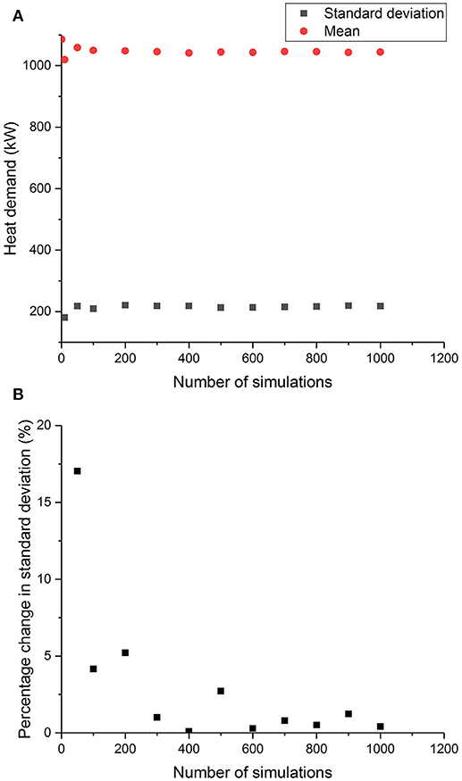
Figure 3. (A) The change in mean and standard deviation with an increasing number of simulations. (B) The percentage change in the standard deviation from trial to trial with an increasing number of simulations.

The results of the Monte Carlo simulations are show in Figure 4. The figure shows the mean heat demand curve, 50th percentile, found over the 1,000 simulations with a black line. The range of percentiles to the extremes of 5th and 95th are denoted by the color bands. Due to software limitations, Figures 4A,B were unable to consider the entire network structure. Instead, the Monte Carlo simulations were run for a typical subnode of the overall model, with the results used to represent the demand experienced in the heat source. Figure 4 does not clearly show the extent of the variation from the mean, therefore more analysis was required. Figure 5 better demonstrates the relation between the input and the output variation for the results from Figure 4. Figure 5 is quantified and shown in Table 3.

FIGURE 4

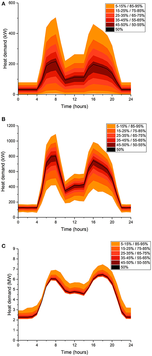
Figure 4. Results of the Monte Carlo simulations for the assumptions in the model, after 1,000 simulations. The mean result, 50th percentile, is shown with a black line. The range of percentiles to the extremes of 5th and 95th are denoted by the color bands. (A) Results of the Monte Carlo simulations for the assumption of each building in an archetype category having the same assumed size (1). (B) Results of the Monte Carlo simulations for the assumption of each building in an archetype category having the same, assumed heat demand profile (2). (C) Results of the Monte Carlo simulations for the assumption that the pipe network travels in the shortest possible straight line distance (3).

FIGURE 5

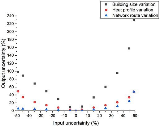
Figure 5. The input and output ranges for the Monte Carlo simulations, showing the assumption of standard building sizes, standard heat demand profiles and a straight line network route.

TABLE 3

Table 3. Input and output uncertainty for the different Monte Carlo studies.

Figure 5 and Table 3 better represent the variation shown in Figure 4 by showing the percentage differences in the power outputs (heat demands) of the different percentile lines. The information used in Figure 5 and Table 3 is a snapshot taken from the afternoon peak at 4 pm showing the current heat demand. Figure 5 and Table 3 show that the Monte Carlo simulation based on the assumption of standard building sizes (1) is highly sensitive to the data used in the simulation. The Monte Carlo simulation is run for a typical network subnode and the results are used to represent the entire network. A 90% variation in the input uncertainty causes 247% variation in the output uncertainty. The assumption of standard building sizes creates a large spread of results and uncertainty, therefore the modeling technique needs to be modified to more accurately quantify the building sizes in the study area. It was unclear from Figure 5 and Table 3 how sensitive the Monte Carlo simulation based on the assumption of standard heat demand profiles (2) was to the data used in the simulation. Figure 5 and Table 3 showed that the Monte Carlo simulation based on the assumption of a straight network route (3) is highly insensitive to the data used in the simulation. A 90% variation in the input uncertainty causes 29% variation in the output uncertainty and a 98% variation in the input uncertainty causes 53% variation in the output uncertainty. The assumption of a straight line network route creates a small spread of results and uncertainty, therefore the assumption of the straight line network route is acceptable for further use.

It was not definitively determined if the assumption of standard heat demands (2) creates an acceptable spread of results. Figure 6 compared the output result distributions to the input distribution found in the literature to provide a better level of understanding.

FIGURE 6

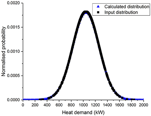
Figure 6. The distribution of the heat demands found by the Monte Carlo simulations of the assumption of an average heat demand profile (2) compared against the distribution of heat demand variations found in the literature, which were used as the inputs into the Monte Carlo simulations.

Figure 6 compares the distribution of the results of the Monte Carlo simulation assessing the assumption of standard heat demand profiles (2) with the distribution in heat demands found in the literature. The Monte Carlo simulation is run for a typical network subnode and the results are used to represent the entire network. The figure shows that the variation due to the assumption is near enough identical to the variation found practically. The matching distributions show that the assumption of standard building heat demands is acceptable for further use.

Thus far, the Monte Carlo analysis was performed investigating one variable at a time instead of globally, where all of the assumptions are varied simultaneously. Global assessment was vital to comprehensively assess the accuracy of the multiple assumptions. As stated, the assumption of standard building sizes was inaccurate, therefore will be omitted from future work. In future work the building sizes (1) will be measured manually, creating a more accurate model. The global assessment now requires the assumptions of standard heat demand profiles (2) and network route length (3) to be done simultaneously as shown in Figure 7.

FIGURE 7

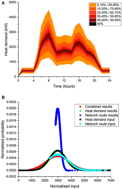
Figure 7. (A) Results of the global Monte Carlo Simulations for the assumption of standard heat demand profiles (2) and network route length (3) after 1,000 simulations. The mean result, 50th percentile, is shown with a black line. The range of percentiles to the extremes of 5th and 95th are denoted by the color bands. (B) The distribution of the heat demand from the global and individual Monte Carlo simulations as well as the distributions of heat demand and network route length as found in the literature.

Figure 7 shows that the results found when assuming that the buildings in the study have a standard heat demand profile (2) and that the network route runs in the shortest possible straight lines (3) have a similar variation to that of building heat demands and network lengths found in literature. Due to the similar variation, it is shown that sensitivity of the results on the input data is acceptable and the assumptions of standard heat demand profiles (2) and straight line network route (3) can be kept in future modeling work.

The modeling technique was altered to remove the assumption of standard building sizes (1), by measuring the buildings in the local area. It was useful to observe the extent that the change to the modeling technique would have had on the results. The modeling process used in Figure 1 was repeated but with accurate building sizes.

Figure 8 quantifies the effects of the changed modeling technique. Figure 8 shows the original model that was generated with the assumed building sizes and the refined model that was generated with measured building sizes. Manually measuring the building sizes increased the heat demand, showing that the assumed building sizes were, on average, smaller than the actual buildings. The increase in the heat demand is likely to be as the assumed building sizes do not accurately account for the number of floors in the buildings. The average variation between the two curves is more than 20% with a peak variation of roughly 40%.

FIGURE 8

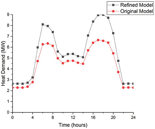
Figure 8. A comparison of the original (assumed building sizes) and refined (measured building sizes) models for local area heat demand.

In the new methodology, there are two possible ways to measure the size of the buildings. The ideal measurement, which would be possible for the non-technical individual at a local authority is to access the building records available. The second technique is to use Google Maps to measure the floor area of a building and use Google Street View to count the number of floors in the building. Using building records should not introduce any error into the work, using Google Maps to measure area has been shown to have errors of 3.54% (Lopes and Nogueira, 2011). The possible errors due to the measurement from Google need to be assessed in a global sensitivity analysis alongside the possible errors from the assumptions of standard building sizes and a straight line network route (Figure 9).

FIGURE 9

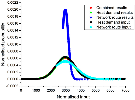
Figure 9. The distribution of the heat demand from the global (including the error from the measurement process) and individual Monte Carlo simulations as well as the distributions of heat demand and network route length as found in the literature.

Figure 9 shows nearly identical results to Figure 7. It is shown that combined global sensitivity analysis, of the two assumptions and the measurement errors, has a similar distribution to that of building heat demands and network lengths found in literature. Due to the similar variation, it is shown that sensitivity of the results on the input data is acceptable and the assumptions of standard heat demand profiles (2) and straight line network route (3) can be kept in future modeling work. In addition it is shown that the risk of the errors from using Google Maps and Google Street View is insignificant and that this measurement technique can be kept in future work.

Conclusions

The hypothesis of this paper proposes a new model that could be used to estimate the hourly heat demand variation of any new district heating network whilst being simple enough that a non-technical staff member could use it. Case studies were investigated to see if the same modeling technique could be used for areas of different population densities. Monte Carlo simulations assessed the accuracy of the assumptions made in the modeling process.

Networks with large population densities were shown to have significantly shorter pipe lengths, resulting in reduced heat losses and installation costs. This may require networks with differing population densities to have differing business cases and incentives in later techno-economic work. Networks with small population densities were shown to be comprised of a large proportion of small domestic customers. In future work, the modeling process will need to be modified to ensure that domestic customers are omitted from the modeling process or, the business case of networks with small population densities may fail. The number, type and location of the customers included in the network, along with the overall pipe length and heat losses in the pipes affects the overall heat demand.

Individually, the assumption of the shortest possible network route (3) and standard building heat demand profiles (2) were found to be acceptable. The network route assumption (3) was shown to be acceptable as a 90% variation in the input uncertainty only causes 29% variation in the output uncertainty. The heat demand assumption (2) was shown to be acceptable as the probability distribution of the results were shown to be identical to the probability distribution in the heat demands of actual buildings. The simultaneous assumptions of a standard heat demand profile (2) and network route (3) were assessed using Monte Carlo simulations. The output distribution of the combined assumptions is similar to the input distribution of the results found in literature, therefore both assumptions can be kept simultaneously in future modeling work.

The assumption of standard building sizes (1) was not acceptable as the output uncertainty was highly sensitive to the input uncertainty. A new modeling technique was proposed, where the building sizes were measured, not assumed, which was shown to significantly alter the modeled hourly heat demand profile. Due to the use of Google Maps and Google Street View to measure the size of the buildings, the new methodology introduces measurement errors of 3.54%. A global sensitivity analysis was run for the measurement errors as well as the assumptions of standard building sizes and straight line network routes. The output distribution of the global sensitivity analysis was similar to the input distribution of the results found in literature, showing that both of the assumptions can be kept in future work. In addition it showed that the errors associated with this measuring technique are minimal and that the new measuring technique can be kept in future work.

Author Contributions

IB was the postgraduate research student who carried out the modeling. PS and SB were the Ph.D. supervisors who directed the research.

Conflict of Interest Statement

The authors declare that the research was conducted in the absence of any commercial or financial relationships that could be construed as a potential conflict of interest.

Acknowledgments

We gratefully acknowledge the Engineering and Physical Sciences Research Council (EPSRC) for funding a CDT Studentship to IB under the Centre for Doctoral Training in Energy Storage and its Applications (EP/L016818/1). PS is grateful for funding from the EPSRC Grand Challenge Network, CO2Chem Network: Establishing the UK as World Leaders in Carbon Dioxide Utilisation (EP/P026435/1). IB is grateful to Robin Idle, H. J. Enthoven and Sons for the provision of energy use data and their experience with the Lead-Acid battery process and to Arup for their help with the heat profile models.

References

Amjady, N. (2001). Short-term hourly load forecasting using time-series modeling with peak load estimation capability. Power Syst. 16, 789–805. doi: 10.1109/59.962429

CrossRef Full Text | Google Scholar

Arup (2007). Level 2 Heat Networks Tool. Manchester: Arup.

Arup (2017). Macclesfield Town Centre Heat Network, Detailed Feasibility Study. Manchester: Arup.

Balcombe, P., Rigby, D., and Azapagic, A. (2015). Energy self-sufficiency, grid demand variability and consumer costs: integrating solar PV, Stirling engine CHP and battery storage. Appl. Energy 155, 393–408. doi: 10.1016/j.apenergy.2015.06.017

CrossRef Full Text | Google Scholar

BEIS (2016). Energy Consumption in the UK. London: Department for Business Energy and Industrial Strategy.

PubMed Abstract

BEIS (2017a). Energy Consumption in the UK. London: Department for Business Energy and Industrial Strategy.

PubMed Abstract

BEIS (2017b). Final UK Greenhouse Gas Emissions National Statistics 1990-2016. Deparment for Business Energy and Industrial Strategy

BEIS (2018). UK CHP Development Map. Department for Business Energy and Industrial Strategy. Available online at: http://chptools.decc.gov.uk/developmentmap/# (Accessed May 10, 2018).

BRE Trust (2015). “Compartment sizes – are they still fit for purpose?,” in BRE Fire Conference 2015 (Watford: Building Research Establishment Trust).

British Steel (2017). Manufacturing. Available online at: http://britishsteel.co.uk/who-we-are/sites-locations/manufacturing/ (Accessed September 28, 2017).

Building Research Association of New Zealand (BRANZ) (2014). Building Energy End-Use Study. Porirua.

Burzynski, R., Crane, M., Yao, R., and Becerra, V. (2011). “Heat demand analysis of residential development in London connected to district heating scheme,” in TSBE EngD Conference (Reading: University of Reading).

Google Scholar

Carbon Trust (2012). Degree Days for Energy Management. London.

Chartered Institution of Building Services, Engineers (CIBSE) (2008). Energy Benchmarks TM46: 2008. London.

Chen, B.-J., Chang, M.-W., and Lin, C.-J. (2004). Load forecasting using support vector machines: a study on EUNITE competition 2001. IEEE Transac. Power Syst. 19, 1821–1830. doi: 10.1109/TPWRS.2004.835679

CrossRef Full Text | Google Scholar

Davies, G., and Woods, P. (2009). The Potential and Costs of District Heating Networks. Pöyry, Oxford.

Department for Communities and Local Government (DCLG) (2014). Rural Population and Migration. London.

Department of Energy and Climate Change (DECC) (2009). Heat and Energy Saving Strategy: Consultation. London.

Department of Energy and Climate Change (DECC) (2013). “The future of heating,” in Meeting the Challenge (London).

Dotzauer, E. (2002). Simple model for prediction of loads in district-heating systems. Appl. Energy 73, 277–284. doi: 10.1016/S0306-2619(02)00078-8

CrossRef Full Text | Google Scholar

ECOBAT (2017). H. J. Enthoven and Sons. Available online at: http://ecobatgroup.com/ecobatgroup-en/facilities/uk/hje/index.php (Accessed November 24, 2017).

EIA (2016). 2012 Commercial Buildings Energy Consumption Survey: Energy Usage Summary. Washington, DC: Energy Information Administration.

European Parliament (2012). Directive 2012/27/EU of the European Parliament and of the council of 25 October 2012 on energy efficiency. Off. J. Eur. Union Direct. 315/1, 1–56. doi: 10.3000/19770677.L_2012.315.eng

CrossRef Full Text

Fang, T., and Lahdelma, R. (2014). State estimation of district heating network based on customer measurements. Appl. Therm. Eng. 73, 1209–1219. doi: 10.1016/j.applthermaleng.2014.09.003

CrossRef Full Text | Google Scholar

Finney, K. N., Sharifi, V. N., Swithenbank, J., Nolan, A., White, S., and Ogden, S. (2012). Developments to an existing city-wide district energy network – Part I: identification of potential expansions using heat mapping. Energy Conv. Manage. 62, 165–175. doi: 10.1016/j.enconman.2012.03.006

CrossRef Full Text | Google Scholar

Finney, K. N., Swithenbank, J., and Sharifi, V. N. (2011). Sheffield Heat Mapping and Feasibility Study of Decentralised Energy. Identification and Impacts of the Potential Expansion of Sheffield's Existing City-Wide District Energy Network using GIS Heat Mapping. SUWIC.

Fonseca, J. A., and Schlueter, A. (2015). Integrated model for characterization of spatiotemporal building energy consumption patterns in neighborhoods and city districts. Appl. Energy 142, 247–265. doi: 10.1016/j.apenergy.2014.12.068

CrossRef Full Text | Google Scholar

Frederiksen, S., and Werner, S. (2013). District Heating and Cooling. Lund: Studentlitteratur.

Google Scholar

Gabrielaitiene, I., Bøhm, B., and Sunden, B. (2007). Modelling temperature dynamics of a district heating system in Naestved, Denmark-A case study. Energy Conv. Manage. 48, 78–86. doi: 10.1016/j.enconman.2006.05.011

CrossRef Full Text | Google Scholar

Gaitani, N., Lehmann, C., Santamouris, M., Mihalakakou, G., and Patargias, P. (2010). Using principal component and cluster analysis in the heating evaluation of the school building sector. Appl. Energy 87, 2079–2086. doi: 10.1016/j.apenergy.2009.12.007

CrossRef Full Text | Google Scholar

Geofabrik (2017). OpenStreetMap. Karlsruhe: Geofabrik.

PubMed Abstract

Goldsim (2011). Goldsim in a Nutshell. Available online at: http://www.goldsim.com/Web/Products/GoldSim/NutshellVideo/ (Accessed February 16, 2017).

Hawkey, D., Webb, J., and Winskel, M. (2013). Organisation and governance of urban energy systems: district heating and cooling in the UK. J. Cleaner Prod. 50, 22–31. doi: 10.1016/j.jclepro.2012.11.018

CrossRef Full Text | Google Scholar

Hawkey, D. J. C. (2009). Will “District Heating Come To Town?” Analysis of Current Opportunities and Challenges in the UK. The University of Edinburgh.

Hayange (2017). Site Officiel de la Ville de Hayange. Available online at: http://www.ville-hayange.fr/ (Accessed September 28, 2017).

Heller, A. J. (2000). Demand Modelling for Central Heating Systems. Lyngby: Technical University of Denmark.

Google Scholar

Heller, A. J. (2002). Heat-load modelling for large systems. Appl. Energy 72, 371–387. doi: 10.1016/S0306-2619(02)00020-X

CrossRef Full Text | Google Scholar

Holmgren, K., and Gebremedhin, A. (2004). Modelling a district heating system: introduction of waste incineration, policy instruments and co-operation with an industry. Energy Policy 32, 1807–1817. doi: 10.1016/S0301-4215(03)00168-X

CrossRef Full Text | Google Scholar

Jie, P., Tian, Z., Yuan, S., and Zhu, N. (2012). Modeling the dynamic characteristics of a district heating network. Energy 39, 126–134. doi: 10.1016/j.energy.2012.01.055

CrossRef Full Text | Google Scholar

Johansson, C. (2010). Towards Intelligent District Heating. Blekinge: Blekinge Institute of Technology.

Google Scholar

Keçebaş, A., Yabanova, I., and Yumurtac,i, M. (2012). Artificial neural network modeling of geothermal district heating system thought exergy analysis. Energy Conv. Manage. 64, 206–212. doi: 10.1016/j.enconman.2012.06.002

CrossRef Full Text | Google Scholar

Kipping, A., and Trømborg, E. (2017). Modeling hourly consumption of electricity and district heat in non-residential buildings. Energy 123, 473–486. doi: 10.1016/j.energy.2017.01.108

CrossRef Full Text | Google Scholar

Lara, R. A., Pernigotto, G., Cappelletti, F., Romagnoni, P., and Gasparella, A. (2015). Energy audit of schools by means of cluster analysis. Energy Build. 95, 160–171. doi: 10.1016/j.enbuild.2015.03.036

CrossRef Full Text | Google Scholar

Larsen, H. V., Bøhm, B., and Wigbels, M. (2004). A comparison of aggregated models for simulation and operational optimisation of district heating networks. Energy Conv. Manage. 45, 1119–1139. doi: 10.1016/j.enconman.2003.08.006

CrossRef Full Text | Google Scholar

Larsen, H. V., Palsson, H., Bøhm, B., and Ravn, H. F. (2002). Aggregated dynamic simulation model of district heating networks. Energy Conv. Manage. 43, 995–1019. doi: 10.1016/S0196-8904(01)00093-0

CrossRef Full Text | Google Scholar

Lim, S., Park, S., Chung, H., Kim, M., Baik, Y. J., and Shin, S. (2015). Dynamic modeling of building heat network system using Simulink. Appl. Therm. Eng. 84, 375–389. doi: 10.1016/j.applthermaleng.2015.03.068

CrossRef Full Text | Google Scholar

Lopes, E. E., and Nogueira, R. (2011). Proposta Metodológica para Validação de Imagens de Alta Resolução do Google Earth para a Produção de Mapas. SBSR.

Lygnerud, K., and Peltola-Ojala, P. (2010). Factors impacting district heating companies' decision to provide small house customers with heat. Appl. Energy 87, 185–190. doi: 10.1016/j.apenergy.2009.05.007

CrossRef Full Text | Google Scholar

Met Office (2015). Derbyshire Dales NNR Hourly Temperature Data. London: Met Office.

Nilsson, S. F., Reidhav, C., Lygnerud, K., and Werner, S. (2008). Sparse district-heating in Sweden. Appl. Energy 85, 555–564. doi: 10.1016/j.apenergy.2007.07.011

CrossRef Full Text | Google Scholar

Noussan, M., Cerino Abdin, G., Poggio, A., and Roberto, R. (2014). Biomass-fired CHP and heat storage system simulations in existing district heating systems. Appl. Therm. Eng. 71, 729–735. doi: 10.1016/j.applthermaleng.2013.11.021

CrossRef Full Text | Google Scholar

Noussan, M., Jarre, M., and Poggio, A. (2017). Real operation data analysis on district heating load patterns. Energy 129, 70–78. doi: 10.1016/j.energy.2017.04.079

CrossRef Full Text | Google Scholar

Nouvel, R., Schulte, C., Eicker, U., Pietruschka, D., and Coors, V. (2013). “CityGML-based 3D city model for energy diagnostics and urban energy policy support,” in Proceedings of BS2013: 13th Conference of International Building Performance Simulation Association (Chambéry), 218–225.

Google Scholar

Olsen, P. K. (2014). Guidelines for Low-Temperature District Heating. EUDP 2010-II: Full-Scale Demonstration of Low-Temperature District Heating in Existing Buildings, EUDP. 1–43.

ONS (2009). Population Estimate for UK, England and Wales, Scotland and Northern Ireland. London: Office for National Statistics.

ONS (2011a). rural and urban areas: comparing lives using rural/ urban classifications. Reg. Trends 43, 11–86. doi: 10.1057/rt.2011.2

CrossRef Full Text

ONS (2011b). QS102EW - Population Density.

ONS (2014). Neighbourhood Statistics. London: Office for National Statistics.

Palsson, H., Larsen, H. V., Bøhm, B., Ravn, H. F., and Zhou, J. (1999). Equivalent Models of District Heating Systems for on-Line Minimization of Operational Costs of the Complete District Heating System. The Technical University of Denmark.

Palsson, O. P. (1993). Stochastic Modeling, Control and Optimization of District Heating Systems. Technical University of Denmark.

Park, T. C., Kim, U. S., Kim, L.-H., Jo, B. W., and Yeo, Y. K. (2010). Heat consumption forecasting using partial least squares, artificial neural network and support vector regression techniques in district heating systems. Korean J. Chem. Eng. 27, 1063–1071. doi: 10.1007/s11814-010-0220-9

CrossRef Full Text | Google Scholar

Parsons Brinckerhoff (2011). A District Heating Utility for the Tees Valley: Study into the Strategic use of Waste Heat and Supply of Private Sector Customers. London.

Pirouti, M. (2013). Modelling and Analysis of a District Heating Network. Cardiff University.

Raab, S., Mangold, D., and Müller-Steinhagen, H. (2005). Validation of a computer model for solar assisted district heating systems with seasonal hot water heat store. Solar Energy 79, 531–543. doi: 10.1016/j.solener.2004.10.014

CrossRef Full Text | Google Scholar

Raine, R. D. (2016). Sheffield's Low Carbon Heat Network and its Energy Storage Potential. The University of Sheffield.

Raine, R. D., Sharifi, V. N., and Swithenbank, J. (2014). Optimisation of combined heat and power production for buildings using heat storage. Energy Conv. Manage. 87, 164–174. doi: 10.1016/j.enconman.2014.07.022

CrossRef Full Text | Google Scholar

Reidhav, C., and Werner, S. (2008). Profitability of sparse district heating. Appl. Energy 85, 867–877. doi: 10.1016/j.apenergy.2008.01.006

CrossRef Full Text | Google Scholar

Sipilä, K. (2011). District Heating for Energy Efficient Building Areas. IEA DHC/CHP Annex IX.

Spoladore, A., Borelli, D., Devia, F., Mora, F., and Schenone, C. (2016). Model for forecasting residential heat demand based on natural gas consumption and energy performance indicators. Appl. Energy 182, 488–499. doi: 10.1016/j.apenergy.2016.08.122

CrossRef Full Text | Google Scholar

Talebi, B., Haghighat, F., and Mirzaei, P. A. (2017). Simplified model to predict the thermal demand profile of districts. Energy Build. 145, 213–225. doi: 10.1016/j.enbuild.2017.03.062

CrossRef Full Text | Google Scholar

Talebi, B., Mirzaei, P. A., Bastani, A., and Haghighat, F. (2016). A review of district heating systems: modeling and optimization. Front. Built Environ. 2:22. doi: 10.3389/fbuil.2016.00022

CrossRef Full Text | Google Scholar

Törnros, T., Resch, B., Rupp, M., and Gündra, H. (2016). Geospatial analysis of the building heat demand and distribution losses in a district heating network. ISPRS Int. J. Geo-Inform. 5:219. doi: 10.3390/ijgi5120219

CrossRef Full Text | Google Scholar

Veolia (2014). Sheffield Energy Recovery Facility. Sheffield. Available online at: https://www.veolia.co.uk/sheffield/sites/g/files/dvc461/f/assets/documents/2014/11/Sheffield_ERF_Brochure_0.pdf (Accessed October 06, 2017).

Wang, J., Zhou, Z., and Zhao, J. (2016). A method for the steady-state thermal simulation of district heating systems and model parameters calibration. Energy Conv. Manage. 120, 294–305. doi: 10.1016/j.enconman.2016.04.074

CrossRef Full Text | Google Scholar

Wang, W., Cheng, X., and Liang, X. (2013). Optimization modeling of district heating networks and calculation by the Newton method. Appl. Therm. Eng. 61, 163–170. doi: 10.1016/j.applthermaleng.2013.07.025

CrossRef Full Text | Google Scholar

Werner, S. (1984). The Heat Load in District Heating Systems. Chalmers University of Technology.

Wilson, I. A. G., Rennie, A. J. R., Ding, Y., Eames, P. C., Hall, P. J., and Kelly, N. J. (2013). Historical daily gas and electrical energy flows through Great Britain's transmission networks and the decarbonisation of domestic heat. Energy Policy 61, 301–305. doi: 10.1016/j.enpol.2013.05.110

CrossRef Full Text | Google Scholar

Wojdyga, K. (2014). Predicting heat demand for a district heating systems. Int. J. Energy Power Eng. 3, 237–244. doi: 10.11648/j.ijepe.20140305.13

CrossRef Full Text | Google Scholar

Zhang, G. B., Patuwo, E., and Hu, M. Y. (1998). Forecasting with artificial neural networks: the state of the art. Int. J. Forecast. 14, 35–62. doi: 10.1016/S0169-2070(97)00044-7

CrossRef Full Text | Google Scholar