Research on Time-Dependent Failure Modeling Method of Integrating Discrete Dynamic Event Tree With Fault Tree

Introduction

Overview of Classical PRA and Dynamic PRA Method

The classical PRA methods, such as Event Tree Analysis (ETA), Fault Tree Analysis (FTA), Reliability block Diagram (RBD) are widely accepted throughout nuclear industry. ET/FT are generally based on static Boolean logic structure. ET is used to inductively model the accident progression to dictate all possible accident sequences based on engineering judgment and thermo-hydraulic analysis. FT is used to deductively model the system failure by a top-down, hierarchical tree to analyze all the possible combinations of failure events. But PRA methodology faces challenges including the treatment of time dependent interactions (accident dynamics) and the propagation of physical process uncertainties to risk.

Dynamic PRA (DPRA) have been developed since 1980s. Under the framework of DPRA, many methods can lead to a more realistic risk assessment for nuclear power plant, originating from Dynamic Event Tree Analysis Method (DETAM; Acosta and Siu, 1992; Siu, 1994), Dynamic Logical Analytical Methodology (DYLAM; Cojazzi, 1996), Dynamic Event Tree (DET; Acosta and Siu, 1993). DPRA evaluates the timing and sequencing of events in accident progression and identifies the failure paths under all possible accident scenarios. DPRA is also treated as simulation-based PRA (Mosleh, 2014), or Integrated Deterministic and Probabilistic Safety Assessment (IDPSA), and related reviews and literatures can be found in the references (Aldemir, 2013; Zio, 2014). Among DPRA methods, DET can partially solve the problem of timing and ordering by coupling the stochastic analysis (reliability) with accident simulation. Along with theoretical research, mature modeling, and computational tools of DPRA have been developed for risk quantification and uncertainty analysis, like Accident Dynamics Simulator (ADS; Hsueh and Mosleh, 1996), Analysis of Dynamic Accident Progression Trees (ADAPT; Hakobyan et al., 2008), Simulation-based PRA (SimPRA; Mosleh et al., 2004), Risk Analysis Virtual Environment (Alfonsi et al., 2017), so as to assist PRA practitioners in improving the modeling and computing efficiency. However, DPRA still suffers from several difficulties:

• Tens of thousands of simulation runs are required, even for only one initiating event, when dealing with issues of complex systems;

• It requires an intensive modeling and expensive computing work compared to classical PRA;

• DPRA generates a massive amount of scenario data and requires a post-processing capability of clustering and data mining.

The first challenge has been partly overcome by time discretization, process discretization, appropriate parameter sampling strategies, branching rules, pruning rules, or leveraging the similar branches. The investigation of the third issue is still in progress, such as the traditional scenario clustering algorithm (Mandelli et al., 2013) and topological clustering algorithm (Maljovec et al., 2016). In addition, the extensive computing problem can be addressed by parallel processing and configuring high-performance computing resource. But for the second issue, a refined simulation model is not required for some components of non-safety systems or supporting systems in DPRA which could reduce the work of modeling and debugging.

Currently, DET is one of the most prospective methods in discrete-time DPRA. DET is similar to traditional ET as it evolves the accident sequences by spawning branch events. However, the difference is that the timing and order of ET accident sequences following an initiating event is predetermined by PRA analysts without any interaction of system responses, while that of DETs are determined “online” by a time-dependent system evolution model and a set of branching rules. In general, DETs are classified into two kinds depending on the treatment of continuous stochastic variables: (1) discretization, such as Discrete Dynamic Event Tree (DDET); (2) sampling-based, such as Monte Carlo Dynamic Event Tree (MCDET; Kloos and Peschke, 2006) DDET discretizes continuous aleatory variables (e.g., failure time or recovery time of equipment, operator response time, etc.) into various branches, while MCDET adopts Monte Carlo sampling with DET simulation (with each sample represented by a DDET). This distinction could impact the accuracy of final results when many continuous variables are concerned in the accident sequences.

In recent years, the concept of “hybrid PRA” (Mandelli et al., 2018) has been proposed as a new methodology which refers to the integration of classical PRA into dynamic PRA. The integrated model of DET and FT has been discussed in previous dynamic PRA research. For DET, the conditional probability of header events/frontline system is regarded as a DET branching probability, which accounts for supporting system dependencies and other dependencies among the safety functions in DET simulations, as mentioned in section Treatment of Dependencies in DET Modeling During Accident Analysis. In most of current DET research, the conditional probabilities are estimated offline (Chao and Chang, 2000) before simulation, in order to simplify the DET simulations. An established FT or a known probability distribution is used to represent the DET branch probability of a certain system state. The limitations of conditional probabilities computed offline is that it ignores the dependencies of conditional branch probability on process variables or operating conditions. Thus, it is not numerically accurate enough.

As an alternative, the conditional branch probabilities of DET can be calculated online. It intends to take advantages of classical PRA for treating dependencies and simplifying simulation modeling work (Karanki and Dang, 2016). Even though basic ideas are comprehensible, it is complex to couple the Boolean algorithms and probabilistic calculation with dynamic accident progression. Simulation Code System for Integrated Safety Assessment (SCAIS; Ibánez et al., 2015; Izquierdo et al., 2017) is one of such DET computational tools, but the consideration of how to calculate the conditional probability online in DET simulation is not thoroughly discussed, especially when the branch probability is time-dependent or effected by process variables. Also, this issue is not clearly clarified in other DET software tools.

Goal of This Paper

The objective of this paper is to investigate how to incorporate classical PRA models into simulation-based PRA in a consistent manner. It addresses a new framework of risk quantification of accident scenarios. The integration method points out how to treat time-dependent interactions of accident dynamics including random failures, temporal failure events, system configuration changes, and physical process parameters explicitly. Unlike most of DET previous literatures, this paper does not estimate the time-dependent conditional branch probabilities offline before DET simulation but intends to update FT online in order to obtain DET simulation results more realistically. So, the issue of time-dependent failure modeling is illustrated including:

• From the point of the reliability analysis, the availability of a component is decreasing with operating time, which gives rise to a time-dependent failure probability. It is generally treated as the probability of basic events related to the state duration, with consideration of system configuration changes.

• The dynamic accident progression of a scenario is influenced by the timing and order of events, so the failure probability of a system has temporal relations with the events.

The paper is organized into the following five sections. The mathematical explanation of integration FT into DET with time-dependent and condition-dependent characteristics is illustrated in section Mathematical Basis of Integration Method. The treatment of potential dependencies in DET modeling and their effect of the DET branch probability is presented in section Treatment of Dependencies in DET Modeling During Accident Analysis. Section Integration Method of FT into DET focuses on technical solutions of time-dependent updating, system configuration updating and temporal relations of failure. Finally, a simplified case is provided for demonstration in section Case Study.

Mathematical basis of integration method

The PRA analysis which describes the failure events of a system or equipment is characterized by specific state, process of state transition, while the mechanics simulation of system provides a time-dependent system response of operating parameters during accident evolution. The corresponding control logic is required in Technical Specification, Accident Procedures, etc. From an integrated point of view, an integrated model is developed which couples probabilistic risk analysis with plant condition analysis.

The system state at time t in phase space is characterized by a set of continuous variables and a set of discrete variables as shown in Figure 1. Generally, the continuous variables refer to process variables that have evolved with time, such as pressure and temperature. The discrete variables mainly represent stochastic behaviors such as the random failure of components, uncertainty in the initial and boundary conditions, uncertainty of the system model, etc.

FIGURE 1

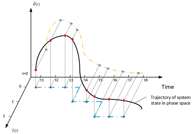
Figure 1. The trajectory of system state in phase space.

The state of system $\overrightarrow{S}(t)\mathrm{\text{=}}\left[\overrightarrow{\theta }(t),\overrightarrow{c}(t)\right]$ can be described by the following equations (Rabiti et al., 2013),

$\begin{array}{ll}\{\begin{array}{ll}\frac{\partial \overrightarrow{\theta }(t)}{\partial t}=\Xi (\overrightarrow{\theta }(t),\overrightarrow{c}(t),t)\hfill & \hfill \\ \hfill & \hfill \\ \frac{\partial \overrightarrow{c}(t)}{\partial t}=\Gamma (\overrightarrow{\theta }(t),\overrightarrow{c}(t),t)\hfill & \hfill \\ \hfill & \hfill \\ \overrightarrow{\theta }(t_0)\text{=}{\overrightarrow{\theta }}_0\hfill & \hfill \\ \hfill & \hfill \\ \overrightarrow{c}(t_0)\text{=}{\overrightarrow{c}}_0\hfill & \hfill \\ \hfill & \hfill \end{array}& (1)\end{array}$

Where $\overrightarrow{\theta }(t)$ describes the NPP status vector of operating parameters, such as the primary pressure and temperature. $\overrightarrow{c}(t)$ is a vector of discrete states for all components, such as operating or failure state, valve open or closed. It is also named as system configuration, i.e., possible combinations of component state. Ξ represents the simulation model of system, which is used to calculate continuous variable, especially operating parameters response. Generally, Ξ is a multi-physics and multi-scale model of thermal-hydraulic, neutronics, material aging, etc. Γ is a time-dependent function of equipment state transitions. It describes the randomness of component states as a probability function. Meanwhile, it is regulated by the control logic (e.g., setpoint values) of a system in operating procedures. For instance, if the water level of pressurizer exceeds an opening threshold, the relief valve is required to action from closed to open.

For a continuously operating device, the time-dependent failure probability can be described by Equation (2).

$\begin{array}{ll}\begin{array}{l}F(t)=P(u<t)\hfill \\ =1-\exp (-{\displaystyle {\int }_0^t\lambda (u)du})\hfill \end{array}& (2)\end{array}$

Where λ(t) is the failure rate of component, t is working time.

The reliability method used in classical PRA is “failure-based reliability” modeling. In this method, the accumulation of failure time and other information are required. Furthermore, a priori life probability function should be determined, and the parameters of probability function should be quantified based on the collected failure data. As a result, the failure-based reliability model is developed to evaluate the remaining lifetime and reliability level of components. Basically, all the failure modes can be classified as traumatic failures and degradation failures. The basic assumption of failure-based reliability modeling is that all failures occur at an instant or in a short period of time. According to this rule, all the failure modes can be regarded as traumatic failures. However, this rule is not always correct because 70–80% of failure modes of mechanical components belongs to degradation failures.

Concerning traumatic and degradation failures, the research on failure probability related to operating environment of system is called “performance-based reliability.” It is based on performance-based reliability indicators (PBRI), that is, some of the operating variables which are strongly dependent on reliability.

In fact, reliability parameters are usually both condition-dependent and time-dependent, where $X_t\text{= }{[\text{ }{X}_1,X_2,\mathrm{..},X_m]}^{\text{T}}$ is the vector of PBRI. The failure rate function equipment λ(t, X_t) is defined as

$\begin{array}{ll}\lambda (t,{\text{X}}_{\text{t}})\text{=}\frac{f(t,{\text{X}}_t)}{R(t,{\text{X}}_t)}& (3)\end{array}$

Where f(t, X_t) is the probability density function of equipment, R(t, X_t) is the reliability function of equipment.

Under different performance levels X_t1 and X_t2, it is assumed that the ratio of failure rate is a constant related to performance level at time t. Then the relationship between failure rate and performance level is in accordance with the Proportional Hazard Model (John, 2008)

$\begin{array}{ll}\frac{\lambda (t,{\text{X}}_{\text{t1}})}{\lambda (t,{\text{X}}_{\text{t2}})}\text{=}C& (4)\end{array}$

Where C is a constant which does not vary with time, only influenced by performance level.

Then the traumatic failure rate λ(t, X_t) can be split into two parts as

$\begin{array}{ll}\lambda (t,X_t)\text{=}{\lambda }_{r0}(t)\text{g}(\text{β},X_t)& (5)\end{array}$

Where λ_r0(t) is the baseline failure rate which is a function of time alone, independent of performance variables. β is a vector of coefficients, each element of which indicates the importance or weight of each variable of X_t. g(β, X_t) is a function of performance variables X_t and coefficient β.

To be simplified, a general form considered for g(β, X_t) is

$\begin{array}{ll}\text{g}(\text{β},X_t)\text{=exp(}{\displaystyle \sum _{i=1}^m{\beta }_i}{X}_i)& (6)\end{array}$

Where X_i is an element of $X_t\text{= }{[\text{ }{X}_1,X_2,\mathrm{..},X_m]}^{\text{T}}$, i = 1, 2, …, m.

Therefore, the unavailability function is described as

$\begin{array}{ll}\begin{array}{l}F(t,X_t)=P(s<t|X_t)\hfill \\ =1-\exp (-\text{exp(}{\displaystyle \sum _{i=1}^n{\beta }_i}{X}_i){\displaystyle {\int }_0^t{\lambda }_{r0}(s)ds})\hfill \end{array}& (7)\end{array}$

Equation (7) points out the FT model of continuous running components is not only related with the system configuration and state duration, but also dependent on the variation of process variables. However, it is quite difficult to quantify the value of β_i corresponding to X_i in engineering practice because of the coupling relationship between failure mechanism and performance level, especially for mechanical components.

Treatment of dependencies in DET modeling during accident analysis

In order to simplify the DET modeling process, one of the generic modeling strategies is to select failures of pivotal functional events/frontline systems as the headers of DET branch. DET branch probabilities are supposed to account for dependencies and configuration consistency among the safety functions in DET simulations. The dependencies here include the functional dependency, configuration dependency, component failure dependency, and human error dependency. Other dependencies are explicitly accounted for as the event tree headers, such as the correlations between functional events, correlations among initiating event and each functional events.

The functional dependency in PSA practice mainly refers to the supporting system dependencies among functions which result from shared supply and shared components. The safety systems in NPP have shared electrical power, water supply, and cooling systems. In terms of the “Small DET- Large FT” strategy, the unavailability of supporting systems are modeled as common modules of FT, and treated by quantitatively determining the Minimal Cut Sets (MCS) of each sequence. Also, it is not recommended to be explicitly modeled in DET headers, so as to reduce the number of branches. In addition, the operating conditions and state duration of subsequent functioning systems depend on the continuous operating time and performance level of previous safety systems, the response time of required human actions. These timing and conditions are not considered in the classical ET method.

The configuration consistency means that the unavailable components during the accident remains irreparable until the end of simulation time except for offsite power recovery and EDG recovery. The component failure dependency includes the common cause failure (CCF) of components due to similar design defects, process of fabrication or installation, procedures of operation. CCF events have been employed in the PRA model to represent all possible dependent reasons in ET/FT logical models. Some of CCF methods (NUREG/CR-6268, NUREG, 2007) have been applied in PRA modeling, such as β Factor Model, Multiple Greek Letter (MGL) model and Alpha Factor Model. Another type of component failure dependency is sequential failure (SF) of components, which are normally not explicitly considered in classical PRA, except for employment of some dynamic gates, such as Priority-AND Gate (PAND) Gate, Sequence Enforcing Gate (SEQ). Accordingly, the CCF modeling and SF modeling also need to be considered in DET.

As for the human error dependency, in order to simplify the analysis and calculation process, the correlation between human tasks is usually divided by specifying correlation parameters. In addition, the probability of human error in the task should be modified according to the level of correlation.

Integration method of FT into DET

The INL report (Mandelli et al., 2018) explains how the four main classical PRA methods (Markov, ET, FT, and RBD) is extended to time domain. It gives a case study of the LBLOCA accident to demonstrate how FTs can be linked to RELAP5-3D PWR model and RAVEN Ensemble Model, and compares the classical PRA results with dynamic PRA. The considered FTs of LBLOCA are of four main frontline systems, i.e., Accumulator (ACC), Low Pressure Injection (LPI) System, High Pressure Injection (HPI) System, and Low Pressure Recirculation (LPR) System. For each frontline system, basic events indicate the states of trains or components, such as failure on demand, unavailable due to test or maintenance, fail to open, etc. Monte-Carlo sampling method is employed to sample the set of stochastic parameters from the calculated probability distribution of basic events. As a result, a series of simulations are generated for the calculations of safety parameters. However, the probability distributions of basic events have been determined before RELAP5-3D simulation. Although the “mission time” of safety system is not illustrated, it is usually set as 24 h in classical PRA practice conservatively. Thus, the “mission time” of safety system is not equivalent to the commissioning time of a frontline system for mitigating accident successfully. Besides, all the branch conditions and configuration changes are embedded into the simulation. The states and state delay time of ACC, HPI, LPI, and LPR are mapped into RELAP5-3D input file. Therefore, INL integration method is only applicable when the probability distribution of stochastic parameters would not change with process variables, that is, the failure probability of a component/train is “failure-based,” not “performance-based.”

To further extend the integration method of INL, a combination of DDET and FT is proposed with online calculation of conditional branch probability. The basic assumptions of events' behaviors are:

• Once an event occurs, it becomes logically true thereafter.

• The occurrence of an event is instantaneous, such as the transition from false to true,

• All the components are available and irreparable.

Key Technical Issues of Integration Method

System Configuration Changes Due to Branching Rules

Unlike ET, DET is more flexible to allow for multiple branches, if necessary. The branching rules include:

a. The branching occurs whenever the control logic is fulfilled, setpoint values of system are exceeded or operator actions are required. These requirements mostly exist in NPP design, Technical Specifications, and Emergency Operating Procedures. The system parameters evolve with time for each branch. Based on the possible outcome of system response, new demands of frontline systems or human actions are generated to perform safety functions. Thus, descendent branching occurs and generates more scenarios because of different events at different timings.

b. The branching occurs when a certain system parameter (such as operating time of a component or internal pressure of a pipe) exceeds the value corresponding to a probability threshold of a known probability distribution. This probability threshold rule is used for operating failures and demand failures. Besides, in engineering practice, it is common to discretize the distribution by the number of available components/trains. For instance, the probability distribution of LPI system is divided into four sections (<5, 5–50, 50–95, >95%).

c. The branching occurs at a specific failure timing by Monte-Carlo sampling or user-defined timing. This rule mostly exists in MCDET.

The state transition of components determines the system configuration of each branch. For probabilistic analysis, it is required to update logic values of events. For the simulation model of the system response, a set of mapping rules of the functional failure simulation are proposed to update the states of spawned branch nodes according to system configuration changes. The mapping rules transfer the state of components into related operating parameters or control variables. The implementation of such rules is introduced as follows. Firstly, the main functional requirements of the system should be identified to obtain a set of system parameters that characterize its functional state. Secondly, the function(s) of the system is decomposed according to a hierarchical level of system-subsystem-component. Thirdly, FMEA analysis for each of the main functional components is carried out to determine the characteristic parameters of components. Equivalently, the system simulation model can be updated using these characteristic parameters or control variables in case of configuration changes. For example, Component Cooling Water (CCS) System is designed to provide adequate cooling water for certain systems with nominal temperature and flow rate. It is composed of two redundant trains A and B. Each train has two redundant 100% CCS pumps and two 50% heat exchangers (HX), one tank and related valves. In normal conditions, CCS operates with one train. To ensure the safe operation, the normal states of the components/system are guaranteed by a set of characteristic parameters in Figure 2, thereby one of the ways to update the system configuration in simulation model is shown in Table 1.

FIGURE 2

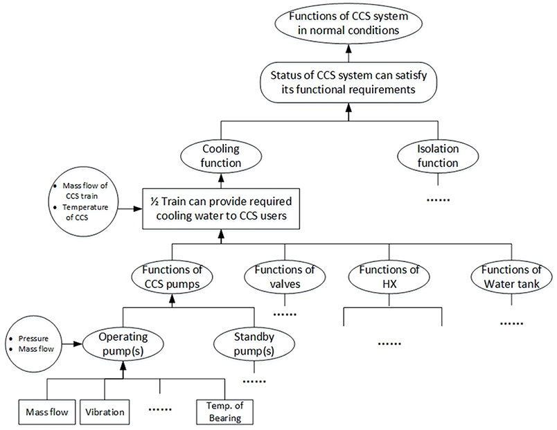
Figure 2. Characteristic parameters of CCS system.

TABLE 1

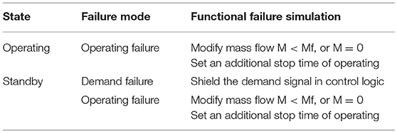
Table 1. Mapping rules of functional failure simulation for CCS pump.

Time-Dependency on Conditional Branch Probability

Unlike ET, the functional demand of a header event/frontline system in DET is determined by a simulation model, not by predetermined success criteria of system. Furthermore, the actual operating time between DET nodes is determined according to actual accident progression, which is noted as “online.” In this view, the conditional branch probability can be understood as “the probability of a specific system configuration, given a set of history events under an accident scenario.” For discrete variables of safety functions, such as valve open or closed, the probability distribution of demand failure of a component is a Bernoulli distribution. For continuous variables of safety functions, such as operating failures, or human action failures, the probability distribution should be updated including logic values and state duration of events in an accident scenario. The duration of a certain state is from its demand moment to the terminated moment, where “termination” occurs because of exhaustion of water, power, or random failures of components.

The demand failures occur when a component state transfers from a non-functional state to functional state which include:

• Demand to run for pumps, motors, compressors, etc.

• Demand to open or close, for switches, valves, breakers, etc.

Thus, the demand failure probability F_SD consists of two parts:

• Standby failure probability F_S. F_S is a function of standby time and failure rate.

• Failure probability of state transition Q₀, given that it does not fail during standby period.

For online-monitored components, the failure state can be monitored by Digital I&C system of NPP in a quite short period after it occurs. It is guaranteed that the state of component is available when IE occurs. So F_SD can be described by Equation (8) in which t = 0 means the end time of the last periodic test.

$\begin{array}{l}{F}_{SD}(t,T_s|F_{SD}(0,T_s)=0)=F_S(t,T_s|F_{SD}(0,T_s)=0)\\ +Q_0·[1-F_S(t,T_s|F_{SD}(0,T_s)=0)]\\ =1-\exp \left(-{\displaystyle \underset{T_s}{\overset{T_s+t_1}{\int }}{\lambda }_s{}^{\prime }(u)du}\right)\\ +Q_0·\exp \left(-{\displaystyle \underset{T_s}{\overset{T_s+t_1}{\int }}{\lambda }_s{}^{\prime }(u)du}\right)& (8)\end{array}$

Where λ_s(t) is the standby failure rate. T_s is the standby time interval from the last period test to the instant when IE occurs. t₁ is the time when generating the demand of component after IE occurs.

For other non-monitored components, the failure probability is

$\begin{array}{l}{F}_{SD}(t,T_s)=F_S(t,T_s)+Q_0·[1-F_S(t,T_s)]\\ =1-\exp \left(-{\displaystyle \underset{{}_0}{\overset{T_s+t_1}{\int }}{\lambda }_s{}^{\prime }(u)du}\right)\\ +Q_0·\exp \left(-{\displaystyle \underset{0}{\overset{T_s+t_1}{\int }}{\lambda }_s{}^{\prime }(u)du}\right)& (9)\end{array}$

To be conservative, T_s is chosen to be test interval (TI). So Equations (8, 9) can be written as

$\begin{array}{l}{F}_{SD}(t,T_s|F_{SD}(0,T_s)=0)=1-\exp \left(-{\displaystyle \underset{TI}{\overset{TI+t_1}{\int }}{\lambda }_s{}^{\prime }(u)du}\right)\\ +Q_0·\exp \left(-{\displaystyle \underset{TI}{\overset{TI+t_1}{\int }}{\lambda }_s{}^{\prime }(u)du}\right)& (10)\end{array}$

$\begin{array}{l}{F}_{SD}(t,T_s)=1-\exp \left(-{\displaystyle \underset{{}_0}{\overset{T_I+t_1}{\int }}{\lambda }_s{}^{\prime }(u)du}\right)\\ +Q_0·\exp \left(-{\displaystyle \underset{0}{\overset{T_I+t_1}{\int }}{\lambda }_s{}^{\prime }(u)du}\right)& (11)\end{array}$

The operational failure means the failure of a component whose functions should be maintained. It includes:

• Continuous running failures of active components, such as pump, motor, etc.

• Failures to maintain an open/closed state for switch-type components.

• Some components without state transition, such as heat exchangers.

• Some failures potentially occurred at any time, no matter what the state is, such as leakage of valves.

For an irreparable component, the time-dependent probability model related to a certain DET branch is listed in Table 2. It illustrates the updating process of logic value and probability when state transition occurs in DET branches.

TABLE 2

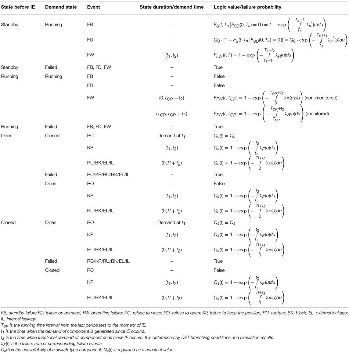
Table 2. Failure probability of time-dependent events.

The Temporal Failure

The temporal failure relationship is dependent on the timing and order of events. It is assumed that all the failures occur instantaneously. If X and Y are both events which lead to system failure, the temporal failure relationship of two events X and Y can be summarized as:

a) X occurs first, then Y occurs, or Y occurs first, then X occurs. In other words, one of the failure events occurs before another.

b) X and Y occur simultaneously.

c) One of the events occurs while another doesn't occur.

Obviously, the static fault tree cannot directly describe all of temporal relationship with AND or OR Gates. The issue of temporal failure is focused on standby redundant systems, basically sequential failures. There are two common kinds of sequential failures (Zhang et al., 2018):

• When one of the redundant units/trains fails, standby unit/train actuates and continues running. The sequence-dependent failure usually occurs between control/monitoring units and redundant units in a standby train. The failure order of two units determines whether the system fails or not, represented by PAND Gate.

• For some standby redundant units/trains, failure of the first operating unit is a prerequisite of the second operating unit to fail. It is called condition-dependent failure, represented by CAND Gate.

In accident analysis of NPP, the temporal failure relations are characterized by supporting systems, not by safety systems, because the actuating conditions of different trains in a safety system are the same, as well as the demanding requirements. In general, all the available trains of safety systems are demanded to operate after actuation. So, switching among redundant trains is considered for supporting systems. For instance, the sequential FT of CCS is shown in Figure 3.

FIGURE 3

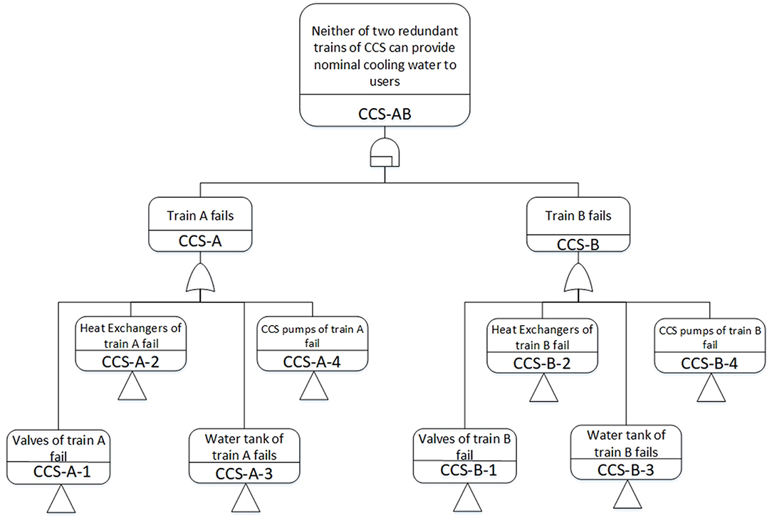
Figure 3. Sequential FT of CCS system.

Under some circumstances, the order of events is more important than the exact moments when they occur. The sequence value, like in Pandora (Walker and Papadopoulos, 2009), is used to establish a set of temporal laws, and analyze qualitatively to obtain Minimal Cut Sequences (MCSQ). This process can identify some sequential contradictions which reduces the complexity of hybrid model with dynamic and static gates. Table 3 represents sequence values, temporal relations, and failure probability for logical gates of dynamic fault tree and static fault tree.

TABLE 3

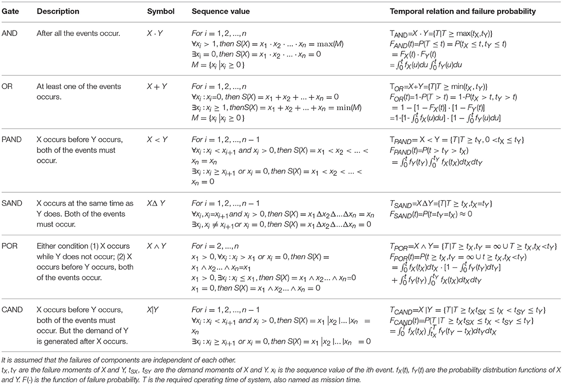
Table 3. Temporal relations of failure in logical gates.

Procedures of Integration Method

In static FT, events are represented by Boolean variables with logical values (True, False, and Normal) and probability value. FT logic gates are treated as operators. In order to ensure that the timing relationship of different variables is not hindered by FT model in accident scenarios, this paper proposes “mission-based DDET” as a framework in consideration of timing and probability characteristics. “Mission phase” is determined according to different functional requirements of safety functions and triggered by branching conditions. In other words, a mission phase will not change until a new event occurs or ending conditions is reached.

To illustrate the modeling and updating process of mission-based DDET, it is necessary to define the state of each branch. Each branch corresponds to a specific state of safety systems, or human actions. The response of safety functions could be represented by either discrete or continuous variables.

1) For the discrete stochastic variables, the number of possible system states is finite, so the DDET simulation runs to implement is finite. For example, the demand states might be success on demand and failure on demand. Besides, it is common practice to spawn branches with the consideration of how many available trains successfully start-up on a demand, such as the number of ECCS available trains (0/3, 1/3, 2/3, 3/3). Thus, the DDET allows non-binary branching nodes and a specific FT is constructed for a branch state.

2) For the continuous stochastic variables, it is characterized with a continuous probability distribution, such as the response time of operator actions, failure time of components. In DDET method, it is assumed that the response time of continuous safety function is described as a known cumulative distribution function (CDF(t)). Then according to a user-defined percentile/probability threshold, CDF(t) could be discretized into several intervals. The occurrence probability of a representative point for each interval is regarded as branch probability.

The progression of Mission-based DDET is shown in Figure 4. The skeleton framework of system failures is developed by DDET method while the failures of subsystem and components are represented by FTs. Each node of DDET is labeled by a specific branching event. Therefore, given previous nodes, the conditional branch probability could be calculated by the analysis of FTs. However, this is different from the traditional PRA method which predetermines the success criteria of systems offline. The mission-based FTs are used to calculate the probability of a specific state in a time interval, under the specific performance level. They are mostly used to model operating failures and obtain “the conditional probability of specific state or specific action from the last DET node to this DET node,” such as the conditional branch probability of S2 system between Node c and Node d, given only one available train. Meanwhile, the timing and order of standby redundant trains switching is considered in FT modeling process on the basis of the temporal failure relationship as described in section The Temporal Failure. DDET evolves with time according to the branching rules described in section System configuration changes due to branching rules. As a result, the consequences of accident scenarios are determined by DDET simulation results such as safety parameters of interest and the probability of accident scenario is determined by the conditional branch probability.

FIGURE 4

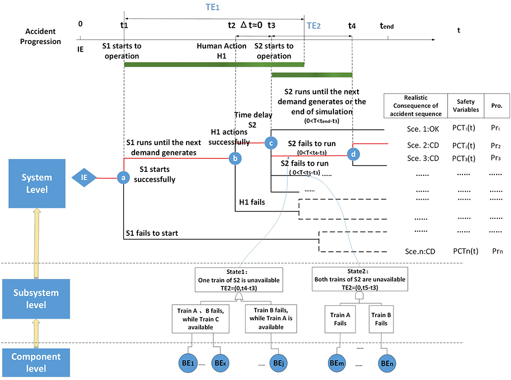
Figure 4. Hierarchical structure of integration FT into DET.

The procedures of DDET simulation coupled FT is shown in Figure 5. After the initialization of DDET simulation, the calculation of simulation model is performed at each discrete time step. The response of process variables, safety components and operator actions are examined, in order to judge whether branch conditions occurs. If one of the branch conditions is satisfied, the process parameters and system configuration of this node are recorded. After that, time-dependent probability updating is performed as described in section Time-Dependency on Conditional Branch Probability and new branches are triggered. For the sake of simplicity, only binary branch is generated in this paper. Then the system configuration updating of failure branches is carried out. On the one hand, the FT of failure branch is updated as described in section Time-Dependency on Conditional Branch Probability. On the other hand, process variables and control variables are updated in the simulation model, as required by mapping rules of functional failure simulation in section System Configuration Changes Due to Branching Rules. But configuration updating is not required for successful branches. After this updating process is completed, each new branch will restart the simulation process, and continues the above procedures until any terminating conditions of simulation is reached. Finally, simulation results are output which include time response of process parameters and conditional branch probability.

FIGURE 5

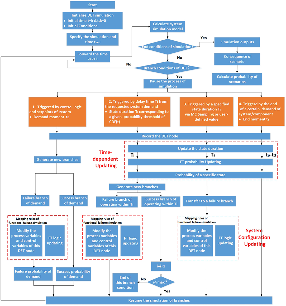
Figure 5. Flow graph of DDET simulation coupled with FT.

In addition, it is recommended to regard the timing and state of each event as another attribute of logical gates, so that the state of upper level can be estimated in advance under some circumstances. To a large extent, it can prejudge some of system responses in this way, thereby simplifying the system simulation model.

Case study

A simple case of a typical PWR with two loops is used for demonstration in this section. The initiating event is Large Break of Loss-of-Coolant Accident (LB-LOCA) on cold leg. The range of break size is from 400 cm² to double-ended guillotine break. In the earlier period, the reactor suffers a sub-cooled blowdown due to the sudden break on cold leg. The pressure of primary system drops dramatically from 15.5 to 12.74 MPa, which triggers the reactor to trip.

When the primary pressure falls to 13.0 MPa, ECCS system is actuated. To complement the large amount of coolant inventory, ECCS system including HPI, LPI, and ACC. ACC automatically actuates at the beginning of the transient accident. When the reactor coolant system pressure drops below 4.91 MPa, the N₂ in ACC automatically injects boron water into the reactor coolant system under the pressure drop of N2 inside. LPI keeps injecting the cooling water with boron from the Refueling Tank to the reactor vessel when the primary system pressure drops below 0.98 MPa, until the low level (2.26 m) of Refueling Tank is reached. The pressure and temperature of containment goes up after the transient accident occurs. When the pressure of containment increases to the setpoint value of 0.149 MPa, then Reactor Containment Spray (RCSS) System actuates to cool down the containment. The large amount of coolant leaked from the primary pipe and the cooling water injected are all collected in the bottom of containment. In order to continue cooling down the reactor, the water source of LPI and RCSS changes to the sump, noted as LPI recirculation mode and RCSS recirculation mode.

Table 4 is the steady state parameters of NPP (Ouyang, 2000). Table 5 lists the timeline of accident progression in Final Safety Analysis Report. Some of the possible scenarios are illustrated in the ET model, as shown in Figure 6, but it cannot cover all the possible scenarios. The progression of accident was modeled with RELAP5/Mod3.1 program. In order to demonstrate the proposed integration method discussed in section Integration Method of FT into DET, a set of phase-based FTs are coupled with the RELAP5 PWR model.

TABLE 4

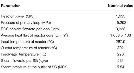
Table 4. Nominal parameters for power operation mode.

TABLE 5

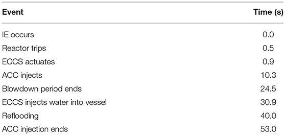
Table 5. Accident sequence of SB-LOCA in FSAR report (Cd = 0.4).

FIGURE 6

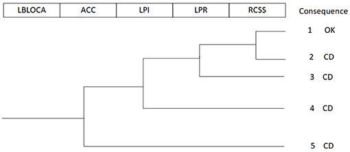
Figure 6. Traditional ET model for a PWR LB-LOCA.

The LPI is taken as an example of conditional branch probability. LPI system is composed of two parallel trains Train A, Train B. Each train consists of one LPI pump and related valves, sensors, etc. In order to compensate the coolant inventory and remove the decay heat from the reactor, the main function of LPI in direct injection mode is to pump the cooling water from the Refueling Tank to the reactor vessel during the first injection period. So, the performance indicator of LPI is mass flow of cooling water.

Assume that:

1) States of a component are binary, i.e., failure and success.

2) The running failure of components are of exponential distribution.

For the direct injection phase of LPI, the nominal mass flow of each LPI pump is M_f kg/h, and then the LPI state of direct injection phase is divided by the availability state of Train A, B. The combinations of available trains are various, as listed in Table 6. In fact, the earlier timing of LPI failure would lead to a decreased total mass flow of LPI. That may result in variation of state duration, which will influence the subsequent branching timing and conditions of LPR, RCSS.

TABLE 6

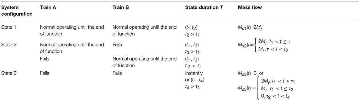
Table 6. State definition by available trains of LPI.

For State 1, it requires Train A and B both work at nominal state, so FTs of State 1 branch (Figure 7) is easily to understand. Assume that the time when actuating LPI is actuated at time t₁, and continuously operates until time t₂, then the conditional branch probability of functional state 1 is defined as “the LPI system maintains to cool down the reactor from Refueling Tank during the period of t₁ to t₂, with the required mass flow of 2^*M_f.” Thus, the FTs of State 1 is constructed with LHIA0100 and LHIA0200 via OR gate. The conditional probability of State 1 branch is

$\begin{array}{ll}\begin{array}{l}P(M_{s1}(t))=1-F(LHIA0000)\hfill \\ =P\{M_{A1}(t)=M_f{\displaystyle \cup M_{B1}}(t)=M_f\}\hfill \end{array}& (12)\end{array}$

Where M_A(t), M_B(t), M_s(t) are the characteristic parameters of Train A, Train B of LPI system.

FIGURE 7

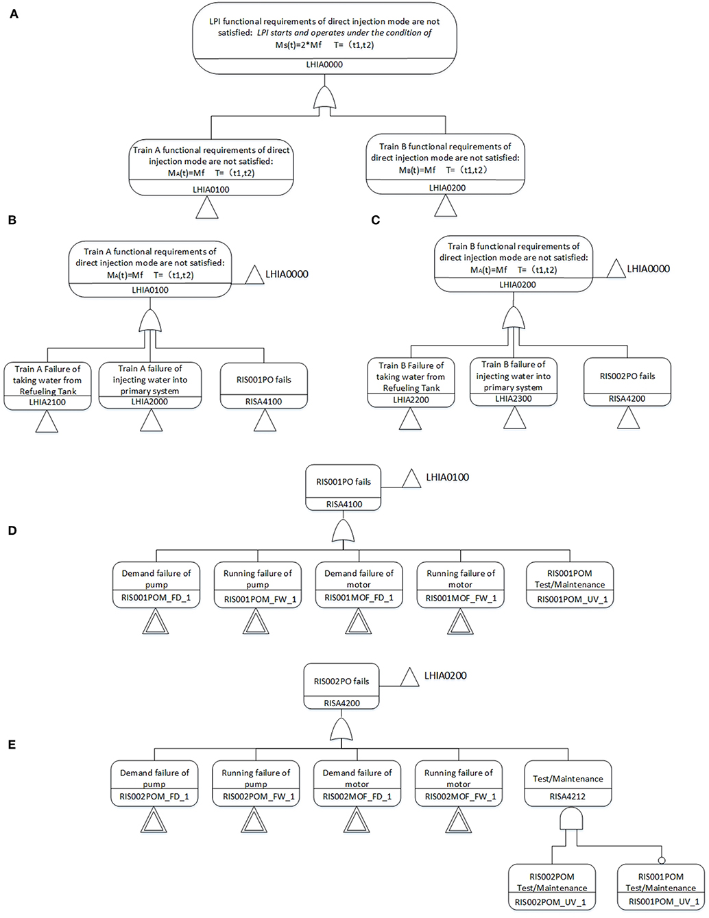
Figure 7. Mission-based FT of LPI.

P(M_s1(t)) is the conditional probability of State 1 branch.

To calculate the conditional probability, a set of reliability parameters (Table 7) is adopted in FTs and others like LHIA 2000, LHIA 2100, LHIA 2200, and LHIA 2300 is treated with transfer gates, whose probabilities are treated with the consideration of CCF failures.

TABLE 7

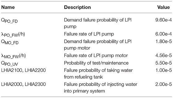
Table 7. Parameters adopted in FTs for LPI system.

The FT of State 2 branch can be automatically reconstructed with LHIA0100, LHIA0200 via NOR gate after time-dependent updating. Similarly, the FT of State 3 branch is reconstructed with the same two gates (LHIA0100, LHIA0200) via AND gate. For the consideration of a conservative simulation output, the system configuration of State 2 is modeled that only one train successfully operation, while the other one is not actuated. Similarly, the system configuration of State 3 is modeled as no mass flow.

$\begin{array}{l}{M}_{A2}(t)=M_f,M_{B2}(t)=\{\begin{array}{l}{M}_f,t_1<t\le \iota \hfill \\ \text{0},\tau <t<t_3\hfill \end{array}\text{or}\\ M_{B2}(t)=M_f,M_{A2}(t)=\{\begin{array}{l}{M}_f,t_1<t\le \iota \hfill \\ \text{0},\tau <t<t_3\hfill \end{array}& (13)\end{array}$

$\begin{array}{l}P(M_{s\text{2}}(t))=P\{M_{A\text{2}}(t){\displaystyle \cup M_{B\text{2}}}(t)\}\\ M_{A3}(t)=0,M_{B3}(t)=0,or& (14)\end{array}$

$\begin{array}{l}{M}_{A\text{3}}(t)=\{\begin{array}{ll}\hfill & M_f,t_1<t\le \iota \hfill \\ \hfill & \text{0,}\tau <t<t_4\hfill \end{array},\\ M_{B\text{3}}(t)=\{\begin{array}{ll}\hfill & M_f,t_1<t\le \iota \hfill \\ \hfill & \text{0,}\tau <t<t_4\hfill \end{array}& (15)\end{array}$

$\begin{array}{ll}P(M_{s\text{3}}(t))=P\left\{M_{A\text{3}}(t)\bigcup M_{B\text{3}}(t)\right\}& (16)\end{array}$

The final results of each LPI branch are listed as Table 8, where T is the state duration obtained from the simulation outputs of a certain accident scenario. Compared to the classical PRA results, the mission time is conservatively chosen to be 24 h of all time-dependent events of LPI in accident scenarios, but the state duration of the integration method are based on simulation results, which varies from each accident scenarios.

TABLE 8

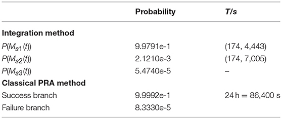
Table 8. Conditional probability of LPI branches.

Conclusion

In Dynamic PRA, the timing and order of events are explicitly considered. But classical FTA/ETA are based on Boolean logic structures with predetermined event sequences and success criteria of systems. This paper aims to incorporate the classical PRA models into simulation-based PRA in a consistent manner. The mathematical basis of integration proves that a time-dependent and condition-dependent model is necessary to describe the relationship among system configurations and state duration, influenced by system response of process variables. To better couple the classical PRA with DPRA, an integration method of FT into DDET is investigated. It analyzes about the treatment of dependencies accounted for DET branch probabilities. To ensure the safety level of NPP, the integration method proposes a mission-based DDET framework to describe the time-dependent interactions between physical phenomena, equipment failures, control logic, and operator actions. Mission-based DDET considers both time discretization and discretization of state transition process based on functional demand. It spawns different branches triggered by branching rules and each FT is modeled for a specific system state. As the operating conditions and state duration are determined by the output of simulation model, the conditional branch probability of DDET in the integration method is calculated online by the automatically reconstructed and updated FTs, according to the time-dependent updating rules and system configuration updating rules. A case study of LPI system in LBLOCA accident is taken to demonstrate the feasibility of this integration method.

For the benefits of this paper, the integrated method can provide a means to identify and characterize a priori unknown vulnerable accident scenarios in the safety analysis of NPP, instead of only binary and predetermined logic by analysts. Besides, it reduces the reliance on expert judgment and simplifying (or overly conservative) assumptions about interdependencies. Furthermore, it provides a way to partially reduce the difficulties of complicated modeling and calculation in DET simulation, which gives support for decision-making in safety margin analysis, modifications of operational procedures, changes of system design.

To improve this study, the future work will focus on how to maintain the accuracy and efficiency of integrated framework, how to balance the time step of simulation process and updating frequency of branch probability, how to enhance the capability of constructing FT automatically in a computational tool. In addition, it is prospective to incorporate the performance-based reliability analysis into this integration method.

Data Availability

All datasets generated for this study are included in the manuscript.

Author Contributions

ZZ instructed and pointed out the problem and proposed to do this research. AX was in charge of and implemented the research to find the reason and solution of the problem. MZ assisted in the case study. HW, HZ, and SC helped to improve and verify the method.

Funding

This study was supported by National Key R&D Program of China on Risk-informed Safety Margin Characterization Technology (2018YFB1900301).

Conflict of Interest Statement

MZ was employed by China Nuclear Power Engineering Co., Ltd.

The remaining authors declare that the research was conducted in the absence of any commercial or financial relationships that could be construed as a potential conflict of interest.

Acknowledgments

The authors also appreciate the dedication from Dr. Xiaomeng Dong.

Abbreviations

ACC, Accumulator; ADS, Accident Dynamics Simulator; CCF, Common Cause Failure; CCS, Component Cooling Water; CDF, Cumulative Distribution Function; DDET, Discrete Dynamic Event Tree; DET, Dynamic Event Tree; DETAM, Dynamic Event Tree Analysis Method; DYLAM, Dynamic Logical Analytical Methodology; DPRA, Dynamic Probabilistic Risk Assessment; ECCS, Emergency Core Cooling System; ET, Event Tree; ETA, Event Tree Analysis; FT, Fault Tree; FTA, Fault Tree Analysis; HPI, High Pressure Injection; HX, Heat Exchanger; IDPSA, Integrated Deterministic and Probabilistic Safety Assessment; INL, Idaho National Laboratory; LBLOCA, Large Break Loss-of-Coolant Accident; LPI, Low Pressure Injection; LPR, Low Pressure Recirculation; MCDET, Monte Carlo Dynamic Event Tree; MCS, Minimal Cut Set; MCSQ, Minimal Cut Sequence; MGL, Multiple Greek Letter; NPP, Nuclear Power Plant; PAND, Priority-AND; PBRI, Performance-based reliability indicator; PRA, Probabilistic Risk Assessment; RAVEN, Risk Analysis Virtual Environment; RBD, Reliability block Diagram; RCSS, Reactor Containment Spray System; SCAIS, Simulation Code System for Integrated Safety Assessment; SEQ, Sequence Enforcing Gate; SF, Sequential Failure; SimPRA, Simulation-based PRA.

References

Acosta, C., and Siu, N. (1992). Dynamic Event Tree Analysis Method (DETAM) for Accident Sequence Analysis, NUREG/CR-5608. U.S. Regulatory Commission.

Google Scholar

Acosta, C., and Siu, N. (1993). Dynamic event trees in accident sequence analysis: application to steam generator tube rupture. Reliab. Eng. Syst. Saf. 41, 135–154. doi: 10.1016/0951-8320(93)90027-V

CrossRef Full Text | Google Scholar

Aldemir, T. (2013). A survey of dynamic methodologies for probabilistic safety assessment of nuclear power plants. Ann. Nucl. Energy 52, 113–124. doi: 10.1016/j.anucene.2012.08.001

CrossRef Full Text | Google Scholar

Alfonsi, A., Rabiti, C., Mandelli, D., Cogliati, J., Wang, C., Talbot, P., et al. (2017). INL/EXT-16-38178 RAVEN Theory Manual and User Guide. Idaho Falls, ID: Idaho National Laboratory.

Chao, C. C., and Chang, C. J. (2000). Development of a dynamic event tree for a pressurized water reactor steam generator tube rupture event. Nucl. Technol. 130, 27–38. doi: 10.13182/NT00-A3075

CrossRef Full Text | Google Scholar

Cojazzi, G. (1996). The DYLAM approach for the dynamic reliability analysis of systems. Reliab. Eng. Syst. Saf. 52, 279–296. doi: 10.1016/0951-8320(95)00139-5

CrossRef Full Text | Google Scholar

Hakobyan, A., Aldemir, T., Denning, R., Dunagan, S., Kunsman, D., Rutt, B., et al. (2008). Dynamic generation of accident progression event trees. Nucl. Eng. Des. 238, 3457–3467. doi: 10.1016/j.nucengdes.2008.08.005

CrossRef Full Text | Google Scholar

Hsueh, K., and Mosleh, A. (1996). The development and application of the accident dynamic simulator for dynamic probabilistic risk assessment of nuclear power plants. Reliab. Eng. Syst. Saf. 52, 297–314. doi: 10.1016/0951-8320(95)00140-9

CrossRef Full Text | Google Scholar

Ibánez, L., Hortal, J., Queral, C., Gómez-Magán, J., Sánchez-Perea, M., Fernández, I., et al. (2015). Application of the integrated safety assessment methodology to safety margins. Dynamic event trees, damage domains, and risk assessment. Reliab. Eng. Syst. Saf. 147, 170–193. doi: 10.1016/j.ress.2015.05.016

CrossRef Full Text | Google Scholar

Izquierdo, J. M., Hortal, J., Sánchez, M., Meléndez, E., Queral, C., and Rivas-Lewicky, J. (2017). Current status and applications of Isa (Integrated Safety Assessment) and SCAIS (Simulation Code System for Isa). Nucl. Eng. Technol. 49, 295–305. doi: 10.1016/j.net.2017.01.013

CrossRef Full Text | Google Scholar

John, O. (2008). Proportional Hazards Regression. New York, NY: Springer.

Google Scholar

Karanki, D. R., and Dang, V. N. (2016). Quantification of dynamic event trees – a comparison with event trees for MLOCA scenario. Reliab. Eng. Syst. Saf. 147, 19–31. doi: 10.1016/j.ress.2015.10.017

CrossRef Full Text | Google Scholar

Kloos, M., and Peschke, J. (2006). MCDET: a probabilistic dynamics method combining monte carlo simulation with the discrete dynamic event tree approach. Nucl. Sci. Eng.153, 137–156. doi: 10.13182/NSE06-A2601

CrossRef Full Text | Google Scholar

Maljovec, D., Liu, S., Wang, B., Mandelli, D., Bremer, P. T., Pascucci, V., et al. (2016). Analyzing simulation-based PRA data through traditional and topological clustering: a BWR station blackout case study. Reliab. Eng. Syst. Saf. 145, 262–276. doi: 10.1016/j.ress.2015.07.001

CrossRef Full Text | Google Scholar

Mandelli, D., Wang, C., Parisi, C., Alfonsi, A., Ma, Z., and Smith, C. (2018). Integration of Classical PRA Models into Dynamic PRA. INL/LTD-18-44955. Idaho National Laboratory.

Mandelli, D., Yilmaz, A., Aldemir, T., Metzroth, K., and Denning, R. (2013). Scenario clustering and dynamic probabilistic risk assessment. Reliab. Eng. Syst. Saf. 115, 146–160. doi: 10.1016/j.ress.2013.02.013

CrossRef Full Text | Google Scholar

Mosleh, A. (2014). PRA: a perspective on strengths, current limitations, and possible improvements. Nucl. Eng. Technol. 46, 1–10. doi: 10.5516/NET.03.2014.700

CrossRef Full Text | Google Scholar

Mosleh, A., Groen, F., Hu, Y., Nejad, H., Zhu, D., and Piers, T. (2004). Simulation Based Probabilistic Risk Analysis Report. Center for Risk and Reliability, University of Maryland.

NUREG (2007). NUREG/CR-6268. Guidelines on Modeling Common-Cause Failure Database and Analysis System: Event Data Collection, Classification, and Coding. Washington, DC: NRC.

Ouyang, Y. (2000). Nuclear Engineering of Qinshan Nuclear Power Plant. Beijing: Atomic Power Press.

Rabiti, C., Mandelli, D., Alfonsi, A., Cogliati, J., and Kinoshita, R. (2013). “Mathematical framework for the analysis of dynamic stochastic systems with the RAVEN code,” in Proceedings of the 2013 International Conference on Mathematics and Computational Methods Applied to Nuclear Science and Engineering-M and C 2013. INL/CON-13-28225 (Idaho National Laboratory).

Google Scholar

Siu, N. (1994). Risk assessment for dynamic systems: an overview. Reliab. Eng. Syst. Saf. 43, 43–73. doi: 10.1016/0951-8320(94)90095-7

CrossRef Full Text | Google Scholar

Walker, M., and Papadopoulos, Y. (2009). Qualitative temporal analysis: towards a full implementation of the Fault Tree Handbook. Control. Eng. Pract. 17, 1115–1125. doi: 10.1016/j.conengprac.2008.10.003

CrossRef Full Text | Google Scholar

Zhang, M., Zhang, Z., and Zheng, G. (2018). Sequential failure modeling and analyzing for standby redundant system based on FTA method. Front. Energy Res. 6:60. doi: 10.3389/fenrg.2018.00060

CrossRef Full Text | Google Scholar

Zio, E. (2014). Integrated deterministic and probabilistic safety assessment: concepts, challenges, research directions. Nucl. Eng. Des. 280, 413–419. doi: 10.1016/j.nucengdes.2014.09.004

CrossRef Full Text | Google Scholar