Mixed Gaussian Models for Modeling Fluctuation Process Characteristics of Photovoltaic Outputs

Introduction

Photovoltaic (PV) power generation is developing rapidly in recent years due to technology maturity and cost reduction (Li Y. et al., 2018a). In 2017, the global PV market grew strongly. Newly installed capacity exceeded 98 GW, an increase of 28.95% over the same period of last year. Global installed capacity has exceeded 402.5 GW, showing a good momentum of development. In the traditional countries such as the United States and Japan, the newly installed capacity reached 10.6 and 7 GW, respectively, which still maintained a strong development momentum. In terms of the development of the PV industry, China has been at the leading level. In 2018, the newly installed capacity of PV power generation exceeded 43 GW in China, down 18% from the previous year, and the cumulative installed capacity exceeded 170 GW. It is expected that the growth of PV installed capacity in China will continue to decrease in 2019, but under the strong demand of emerging countries such as the United States, the European Union and India, it is expected that the global installed capacity will still reach 111.3 GW. However, PV output has the characteristics of randomness and volatility, and the distributed PV distribution points are wide area, a great difference between regions, large fluctuation probability in 1 day, and high difficulty in forecasting. Large-scale access will bring tremendous challenges to the reliability of the power grid operation. In order to better understand the impact of distributed PV grid-connected power systems, it is necessary to study its mathematical model and fluctuation characteristics.

Literature Review

In the aspect of distributed PV power generation estimation method, the literature (Lappalainen and Valkealahti, 2017) uses the mathematical model of irradiance conversion and PV experiment to verify the influence of optical radiation changes caused by cloud movement on the output of PV arrays through a large amount of data. Literature (Cojocariu et al., 2015) established a model of PV cell (PVC) by equivalent modeling, and obtained the working parameters and characteristics of PVC. Literature (Zhao et al., 2017) analyzes the effects of different physical processes on PV output, decomposes the weather physical process into large-scale weather processes and medium-microscale weather processes, and then uses the t location-scale (TLS) distribution to model the random components. However, the classification of physical processes emphasizes meteorological physical factors, ignoring the influence of other components, and the boundary of attenuation modeling is rather vague. Literature (Xia et al., 2017) analyzes the measured output of PV power plants, decomposes the PV output sequence into three components: the ideal output normalization curve, the amplitude parameter and the random component, and uses the amplitude parameter sequence to verify the validity of the TLS distribution function fitting. In summary, the existing analytical methods for the modeling of factors affecting PV output are relatively imprecise, and the division of influencing factors is relatively one-sided, and the statistical analysis of random components is also relatively imprecise. Most of the research focuses on fitting through the more popular single probability density distribution function. It is necessary to determine the distribution function with better fitting to describe the digital characteristics of the random component of PV output.

Contributions of This Paper

The main contributions of this paper are as follows:

(1) A novel solution methodology—to obtain the fluctuation component of PV output accurately a new approach is proposed. According to the theory of the least square method, the theoretical attenuation force closest to the actual output is obtained, and the fluctuation component is obtained by comparing the actual output data with the theoretical attenuation force.

(2) A new mixed Gaussian model—a three-weight mixed Gaussian (TM-G) model based on the expectation maximization (EM) algorithm is proposed for the first time, which can be obtained from the actual data. Compared with common single probability density distribution, the proposed approach gives better fitting effects for the fluctuation component.

(3) The simulation results using actual PV output data in Xichang City, China validate the effectiveness of the proposed approach, which provides an effective way for PV output prediction. The simulation results verify the effectiveness and superiority of the presented approach.

PV Power Generation Model

The basic principle of PV power generation is to convert solar energy into electric energy by using PV panel module according to PV effect. The output of PV power generation is affected by many conditions (Li et al., 2019). The type of components will affect the conversion efficiency of light radiation; the installation method will lead to the difference of the dip angle; while the geographical location, distribution of light resources and topographical conditions are directly or indirectly related to the intensity of light radiation received by PV (Raiti, 2006; Cabrol Nathalie, 2014; Alsadi and Nassar, 2017; Gueymard et al., 2018; Li Y. et al., 2018b; Heinisch et al., 2019), especially the characteristics of distributed PV with “multiple points on multiple sides” leading to the complexity of its model establishment. In this paper, the PV power generation output model has divided into a theoretical output part and a volatility output part according to the available measurement. For the measurable theoretical output part, the model with solar radiation intensity as the reference variable is used to model, and the attenuation theory output model is established by data fitting; the volatility component is the random component, which is an unmeasurable output component. Specifically, the output of the PV output is affected by short-term disturbances.

Define the distributed PV theory output P_thp in the region (Yang and Liu, 2011):

$\begin{array}{ll}{P}_{thp}=P_{stc}\frac{I_a}{I_{stc}}& (1)\end{array}$

where: P_stc is the output of the PV panel under standard conditions (solar radiation intensity I_stc = 1,000 W/m², temperature T_stc = 298 K); I_a is the solar radiation intensity without considering the attenuation component.

According to the above analysis, the solar radiation intensity I_a without occlusion plays a decisive role in the theoretical part P_thp of PV power generation. The total solar radiant energy I_a that can be received on the PV panel mainly includes three parts: direct radiant energy I_b, scattered radiant energy I_d and surface reflected radiant energy I_r. However, since a large part of the ground reflection radiation is ineffective for the silicon cells commonly used today, the surface reflection radiation can be ignored.

Thus, the total solar radiation intensity at t is:

$\begin{array}{ll}{I}_a=I_b+I_d& (2)\end{array}$

Using Equation (2), we can simulate the solar radiation intensity I_a at any time on the earth under the influence of no attenuation component. Substituting I_a into Equation (1) yields an in-region PV deterministic output P_thp.

Direct Radiation Intensity

Direct solar radiation I_b is the main component of solar radiation. The intensity of direct solar radiation in a place can be expressed as:

$\begin{array}{l}{I}_{\text{b}}=0.56S\sin \rho ({\text{e}}^{-0.56M}+{\text{e}}^{-0.095M})\\ \times [1+0.033\cos (\frac{2\text{ }\pi \text{ }(N+10)}{365})]& (3)\end{array}$

where: S is the solar constant, which is about 1,366 W/m²; N is the day of the year; ρ is the solar incident angle, which is the difference between the solar zenith angle θ_Z and the PV panel inclination angle β; M is airmass, related to altitude.

$\begin{array}{ll}M=\{\begin{array}{ll}\frac{P(a)}{P_0\sin {\alpha }_{\text{s}}}\hfill & {\alpha }_{\text{s}}\ge {30}^{°}\hfill \\ \frac{P(a)}{P_0\Gamma }\hfill & {\alpha }_{\text{s}}<{30}^{°}\hfill \end{array}& (4)\end{array}$

$\begin{array}{ll}\text{Γ}=\sqrt{\left[1229+{(614sin{\alpha }_{\text{s}})}^2\right]}-614sin{\alpha }_{\text{s}}& (5)\end{array}$

where: a is the measured ground elevation; P(a) is the measured atmospheric pressure; P₀ is the standard atmospheric pressure. α_s is the local solar elevation angle, which is complementary to the solar zenith angle θ_Z.

Scattering Radiation Intensity

Due to the action of air molecules and aerosol particles, the solar radiation energy is redistributed in various directions to form scattered radiation in a certain regularity. According to the Berlage formula, the solar scatter intensity I_d is (Zhang et al., 2014):

$\begin{array}{ll}{I}_d=\frac{k\left[0.729+0.153E\right]sin{\alpha }_{\text{s}}}{2-2.8ln\frac{0.271-0.153E}{M}}& (6)\end{array}$

$\begin{array}{ll}E={\text{e}}^{-0.56M}+{\text{e}}^{-0.095M}& (7)\end{array}$

$\begin{array}{ll}sin{\alpha }_{\text{s}}=sin\varphi sin\delta +cos\varphi cos\delta cos{\omega }_{\text{s}}& (8)\end{array}$

where: k is a parameter related to air quality. ϕ is the latitude of the area; δ is the declination angle of the sun; ω_s is the solar hour angle.

The solar declination angle varies with the season and is calculated by:

$\begin{array}{ll}\delta =23.45\sin [\frac{\text{ }\pi \text{ }}{\text{2}}(\frac{{\alpha }_1}{N_1}\times \frac{{\alpha }_2}{N_2}\times \frac{{\alpha }_3}{N_3}\times \frac{{\alpha }_4}{N_4})]& (9)\end{array}$

where: N₁ = 92.975 is the number of days from the vernal equinox to the summer solstice; α₁ is the number of days calculated from the vernal equinox date; and so on, N₂ = 93.269, N₃ = 89.865, N₄ = 89.012.

The solar hour angle is represented by ω_s, which increases by 15° every hour due to the earth's rotation. At the same time, the time difference affects the time angle. In the UTC/GMT+08:00 where Beijing time is located, the interval longitude is 120° east longitude. The calculation formula of the time angle ω_s based on Beijing time in a certain area is:

$\begin{array}{ll}{\omega }_{\text{s}}=(12-t)\times 15°+(120°-\psi )& (10)\end{array}$

where: ψ is the local longitude; t is the hour.

Theoretical Output Component Extraction

Theoretical Output Attenuation Model

Actual PV power generation is affected by many practical conditions, and the theoretical output will be attenuated without considering the volatility. The daily attenuation coefficient K_i is used to characterize the attenuation of the PV output. The expression is:

$\begin{array}{ll}{K}_i=\frac{{\displaystyle \sum _{u=1}^n}{f}_i(u)y_i(u)}{{\displaystyle \sum _{u=1}^n}{f}_i^2(u)}& (11)\end{array}$

where: K_i is the attenuation coefficient of the i-th day; y_i(u) and f_i(u) are the measured force values of the u-th sampling point on the i-th day and the PV theoretical output value of the u-th sampling point on the i-th day, respectively; n is the number of sampling points on the i-th day.

The above formula uses the least squares method to find the fitting coefficient with the accurate fitting, so that the sum of the squared residuals of the theoretical output and the measured force is the smallest, that is the optimization problem that matches the theoretical model with the measured data.

Fluctuation Extraction

In addition to the existence of measurable regular components, PV output will also cause random fluctuations in PV output due to short-term disturbances such as temperature changes, cloud and debris, and machine failure. The attenuation theory output combines the effects of the sun-ground motion and the attenuation component, and the difference between the measured output force of the PV and the theoretical output of the attenuation represents the random output component of the PV output.

Based on the measured force data, this paper uses MATLAB as the simulation experiment platform to simulate the wave volume extraction model. This paper selects the historical data of Xichang City (1 d, 15 min/point) on July 20th, 21st, 25th, and August 9th, 2018. Xichang City is located in the plateau of 101°46′~102°25′ east longitude and 27°32′~28°10′ north latitude, with an average elevation of 1,500 m. The selected data sets have different weather and solar radiation intensity, and are represented in different scenarios. Among them, the weather on August 9 was good, the output was stable, and there was no large fluctuation. On July 20, 21, and 25, the PV output fluctuated strongly and the instantaneous power fluctuated greatly. Figure 1 shows the 4-day solar radiation intensity model, and the daily attenuation coefficient K_i is shown in Table 1.

FIGURE 1

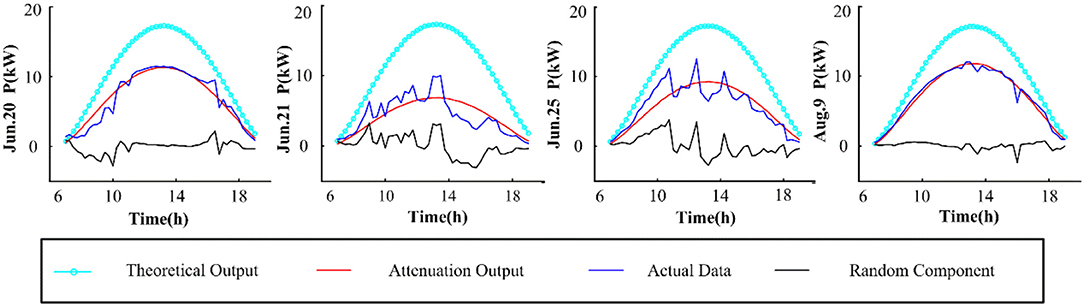
Figure 1. Volatility output component model.

TABLE 1

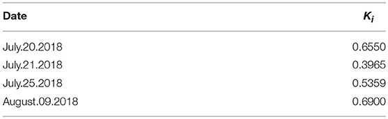
Table 1. Daily attenuation coefficient K_i.

Probability Distribution Fitting of Random Components

Analysis of the Distribution Function Fitting Index

The numerical characteristics of continuous random variables are often described visually through the probability density function. When using the probability density function method to study the digital characteristics of the PV output fluctuation component, the theoretical distribution function with its high fitting matching degree is usually selected. The characteristics can be used to describe the fluctuation characteristics of the PV output. The fitting effect can be quantified by a series of index values. The judgment of the index value on the fitting quality is generally from the angle of error or the perspective of variation correlation. The better the fitting effort, the better the explanatory ability of the independent variable to the dependent variable, the higher the percentage of the change caused by the independent variable is, and the denser the observation point is near the regression line.

The error class indicator is non-negative, and a smaller value of this indicator means better fitting performance.

The mean absolute error (MAE) is the average of the absolute values of the deviations of all individual observations from the arithmetic mean. Its expression is:

$\begin{array}{ll}MAE=\frac{1}{n}{\displaystyle \sum _i}|(g_i-y_i)|& (12)\end{array}$

where: y_i is the functional value of the fitting function for the fluctuation magnitude; g_i is the actual probability value of the fluctuation magnitude;

The root means square error (RMSE) is also called the standard deviation of the regression system. It represents the error between the estimated value of the model and the original value (Lv et al., 2014; Li et al., 2017). The calculation formula is:

$\begin{array}{ll}RMSE=\sqrt{\frac{1}{n}{{\displaystyle \sum _i}(g_i-\overline{y})}^2}& (13)\end{array}$

where $\overline{y}$ is the mean of the actual probability values.

The range of correlation indicators is [0, 1], and the closer to 1, the higher the degree of association between them, the better the fitting effect. The correlation coefficient R is used to describe the correlation between the fitting value of the random component of the PV output power and the actual value. The expression is:

$\begin{array}{ll}R=\frac{\text{Cov}(g_i,y_i)}{\sqrt{\text{Var}(g_i\text{)Var(}{y}_i)}}& (14)\end{array}$

where: Cov() is the covariance function and Var() is the variance function.

The coefficient of determination determines the degree of closeness of the correlation. In multiple regression analysis, the decision coefficient is the square of the correlation coefficient. Define it as R² and calculate it as:

$\begin{array}{ll}{R}^2=\frac{{{\displaystyle \sum _i}(g_i-\overline{y})}^2}{{{\displaystyle \sum _i}(g_i-\overline{y})}^2+{{\displaystyle \sum _i}(y_i-g_i)}^2}& (15)\end{array}$

The adjusted coefficient of determination is the correction of the decision coefficient. As the number of independent variables increases, R² will continue to increase. Therefore, when examining the fitting function of the distribution function model of different number distribution parameters, the distribution must be considered. To achieve the universality of parameter comparison, the variable R_ad is defined to represent the correction decision coefficient (Cui et al., 2016):

$\begin{array}{ll}{R}_{\text{ad}}=1-(1-R^2)\frac{p-1}{p-1-q}& (16)\end{array}$

where: p is the dimension of the data sequence; q is the number of data; the judgment condition of R_ad for the fitting and fitting is the same as R².

However, since R_ad normalizes the decision coefficients of different dimensional data sequences and simultaneously uses the contrast of different dimensional fitting effects, R_ad is generally smaller than R².

Single Probability Distribution Fitting Effect Analysis

To quantitatively describe the probability distribution of random component sequences, this paper analyzes the measured data of distributed PV output and analyzes the effect of the single distribution function model on the probability density distribution characteristics of random components of PV output. Based on the probability density function method to analyze the fluctuation characteristics of PV output, it is necessary to select the appropriate probability density distribution function, and compare the component parameter sequences with the commonly used normal distribution, Logistic distribution and TLS distribution.

To eliminate the influence of the dimension difference between the indicators, the random component data is normalized, and the expression is:

$\begin{array}{ll}{U}_i^{*}=\frac{U_i}{\left|{U_i}_{max}\right|}& (17)\end{array}$

where: U_i is the random component of the PV output.

Figures 2–5 illustrate the stochastic component cumulative probability density distribution function and probability fitting curve of distributed PV output in Xichang City for 2 days. For ease of analysis, August 9th is selected as a typical day with stable outputs; while July 20th is chosen as another typical day with strong volatility. It can be seen from the above figures that the TLS distribution has a good fitting effect using single probability density functions.

FIGURE 2

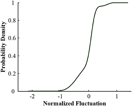
Figure 2. Cumulative probability distribution of random components of PV output in Xichang City on July 20, 2018.

FIGURE 3

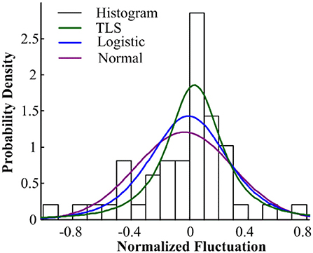
Figure 3. Probability distribution fitting of random components of PV output in Xichang City on July 20, 2018.

FIGURE 4

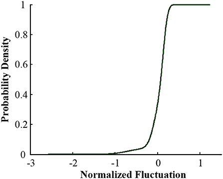
Figure 4. Cumulative probability distribution of random components of PV output in Xichang City on August 9, 2018.

FIGURE 5

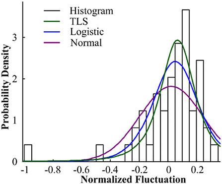
Figure 5. Probability distribution fitting of random components of PV output in Xichang City on August 9, 2018.

To compare the fitting effects of the three distribution functions more clearly, Tables 2, 3, respectively show the index values of the corresponding fitting effects for 2 days.

TABLE 2

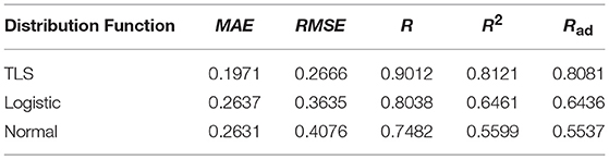
Table 2. Index value of data fitting effect in Xichang City on July 20, 2018.

TABLE 3

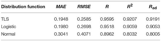
Table 3. Index value of data fitting effect in Xichang City on August 9, 2018.

Comparing the fitting effect index values, it can be seen that the TLS distribution has a relatively good fitting effect on both conditions, and has a lower error coefficient and a higher correlation coefficient. However, even if the TLS distribution fits well in the three popular single distributions, the fit is not ideal from the direction of the data index. TLS distribution can be used to describe the probability density distribution characteristics of PV force fluctuation under the condition that the fitting effect is not exact.

Error Correction

The fitting error of the single probability density distribution function for PV output random variables is large (Cui et al., 2011; Zou et al., 2014; Shen et al., 2015; Yang and Dong, 2016). To reduce the fitting error, a mixed probability density distribution function is introduced to fit.

The mixed probability density function distribution model is obtained by linearly combining multiple single probability distribution models according to different weight. The mixed distribution has a good fitting, flexible shape and strong applicability. The density function of a finite mixed distribution can be expressed as:

$\begin{array}{ll}f(x,\theta )={\displaystyle \sum _{i=1}^n}{\alpha }_{i}g(x)e^{{\displaystyle \sum _{j=1}^k}{P}_j(x)Q_j(\theta )-S(\theta )}& (18)\end{array}$

where:${\displaystyle \sum _{i=1}^n{\alpha }_i=1}$,0≤α_i≤1.

This paper comprehensively investigates the mixed Gaussian distribution model and compares several single distribution functions to obtain the probability distribution function with the best fitness.

In order to obtain the optimal mixed probability density distribution model, a mixed Gaussian probability distribution model is established (Yang et al., 2017; Li et al., 2018). The mixed Gaussian distribution model is a linear superposition of a single Gaussian component, and the goal is to provide a probabilistic model (multimodal probability density distribution) that is more fitting than a single distribution. As a convex function of multiple single distribution combinations, it has a good fitting effect on the probability distribution sequence of PV output random components with convex structure features, and the fitting of the edge samples of the data set is more accurate. The mixed Gaussian probability density distribution function is a latent variable parameter model, and the parameters are solved by EM algorithm clustering. The EM algorithm is a general method for finding the maximum likelihood solution of a probability model with latent variables. The calculation results are stable and accurate. Therefore, it is of certain significance to apply it to the Gaussian mixture probability density fitting analysis of PV output fluctuation. The following formula is a Gaussian mixture model formula.

$\begin{array}{ll}G(x)={\displaystyle \sum _{w=1}^W}{\xi }_{w}N(x|{\mu }_w,\Sigma )& (19)\end{array}$

where ${\displaystyle \sum _{w=1}^W{\xi }_w=1}$ is the mixing factor.

$\begin{array}{ll}N(x|{\mu }_w,\Sigma )={(2\pi )}^{-\frac{i}{2}}{|\Sigma |}^{-\frac{1}{2}}{e}^{-\frac{1}{2}{(x-\mu )}^K{\Sigma }^{-1}(x-\mu )}& (20)\end{array}$

where i is the total number of the used mixed Gaussian distribution, μ is its mean vector, and Σ is its covariance matrix.

To verify the superiority of the mixed Gaussian probability density distribution function, the calculated data of the random component of Xichang City were used for analysis and verification. Firstly, random component data is normalized, and then the data is fitted and analyzed by TLS, normal distribution, double-weight mixed Gaussian distribution (DM-G) and TM-G function models, and the index values are used to compare the fit of them. The data of July 20th and August 9th of 2018 in Xichang City are processed and analyzed. The fitting effect diagrams of the probability components of the volatility components are shown in Figures 6, 7. The weight distribution parameters of the mixed Gaussian distribution model are shown in Tables 4, 6; while the values of the fitting indicators are shown in Tables 5, 7.

FIGURE 6

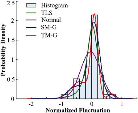
Figure 6. Comparison of probability distribution of volatility components in Xichang City on July 20, 2018.

FIGURE 7

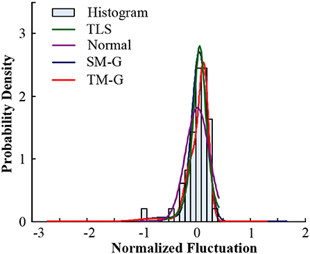
Figure 7. Comparison of probability distribution of volatility components in Xichang City on August 9, 2018.

TABLE 4

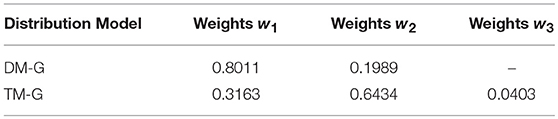
Table 4. Weight value of mixed probability density distribution of Xichang data on July 20, 2018.

TABLE 5

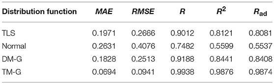
Table 5. Fitting index value of probability density distribution of Xichang data on July 20, 2018.

TABLE 6

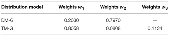
Table 6. Weight value of mixed probability density distribution of Xichang data on August 9, 2018.

TABLE 7

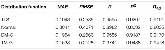
Table 7. Fitting index value of probability density distribution of Xichang data on August 9, 2018.

Comparing the data in the above table, the same type of distribution, the larger the weight, the better the fitting effect. The TM-G is superior to other models in both error angle and correlation angle. In the analysis of PV output fluctuation characteristics based on the probability density function method, the TM-G model is more suitable for analyzing the fluctuation characteristics of PV outputs. However, the fitting accuracy of the three-mixed model has reached 95%. Increasing the number of mixtures will increase the complexity of the model and the training time. Therefore, this work does not continue to explore.

Conclusions

To describe the fluctuation characteristics of PV output, a mixed Gaussian distribution model was proposed to characterize its distribution characteristics. Based on the simulation results of the actual data of Xichang City, China, the conclusions of this paper are as follows:

(1) Based on the actual data, a theoretical model of PV output attenuation is established, and the fluctuation component of PV output is obtained by comparing the attenuated output model with the actual data.

(2) The important finding of this paper is that the TM-G model can be used to fit the fluctuation of PV output accurately. Furthermore, the fitting effect of the TM-G model is more accurate than the single probability distribution, which paves the way for the forecast of PV output.

(3) This work provides a universal methodology for analyzing fluctuation characteristics of PV outputs, which can be used for wide-area distributed PV aggregation analysis.

The future work will focus on the multi-step prediction method of ultra-short-term PV output by using historical output data and correlation analysis. It can provide a reference for the control of PV power plants and the formulation of dispatching plans for power grids.

Data Availability

The datasets analyzed in this manuscript are not publicly available. Requests to access the datasets should be directed to the datasets generated for this study are available on request to the corresponding author.

Author Contributions

ZW and JK: conceptualization. LC: methodology. JK: software. ZW and LC: validation. ZP: formal analysis. ZP, CD, and ZL: resources. CD and ZL: data curation. ZW and ZP: project administration.

Funding

This research was funded by Science and Technology Foundation of SGCC Research and Application of Distributed PV Power Generation Wide-area Monitoring Analysis and Global Output Estimation.

Conflict of Interest Statement

The authors declare that the research was conducted in the absence of any commercial or financial relationships that could be construed as a potential conflict of interest.

References

Alsadi S. Y., and Nassar Y. F. (2017). Estimation of solar irradiance on solar fields: an analytical approach and experimental results. IEEE Trans. Sustain. Energy 8, 1601–1608. doi: 10.1109/TSTE.2017.2697913

CrossRef Full Text | Google Scholar

Cabrol Nathalie A. (2014). Feister UweHäder Donat-Peter. Record solar UV irradiance in the tropical andes. Front. Environ. Sci. 2:19. doi: 10.3389/fenvs.2014.00019

CrossRef Full Text | Google Scholar

Cojocariu B., Petrescu C., and Stefanoiu D. (2015). “Photovoltaic generators-modeling and control,” in 2015 20th International Conference on Control Systems and Computer Science (Bucharest). doi: 10.1109/CSCS.2015.96

CrossRef Full Text | Google Scholar

Cui Y., Mu G., Liu Y., and Yan G. (2011). Spatiotemporal distribution characteristic of wind power fluctuation. Power Syst. Technol. 25, 110–114. doi: 10.13335/j.1000-3673.pst.2011.02.017

CrossRef Full Text

Cui Y., Yang H., and Li H. (2016). Probability density distribution function of wind power fluctuation of a wind farm group based on the Gaussian mixture model. Power Syst. Technol. 40, 1107–1112. doi: 10.13335/j.1000-3673.pst.2016.04.019

CrossRef Full Text

Gueymard C. A., Habte A., and Sengupta M. (2018). Reducing uncertainties in large-scale solar resource data: the impact of aerosols. IEEE J. Photovolt. 8, 1732–1737. doi: 10.1109/JPHOTOV.2018.2869554

CrossRef Full Text | Google Scholar

Heinisch V., Odenberger M., Göransson L., and Johnsson F. (2019). Prosumers in the electricity system-household vs. system optimization of the operation of residential photovoltaic battery systems. Front. Energy Res. 6:145. doi: 10.3389/fenrg.2018.00145

CrossRef Full Text | Google Scholar

Lappalainen K., and Valkealahti S. (2017). Output power variation of different PV array configurations during irradiance transitions caused by moving clouds. Appl. Energy 190, 902–910. doi: 10.1016/j.apenergy.2017.01.013

CrossRef Full Text | Google Scholar

Li F., Li C., and Yan Q. (2017). Photovoltaic output fluctuation characteristics research based on variational Bayesian learning. Electr. Power Autom. Equip. 37, 99–104. doi: 10.16081/j.issn.1006-6047.2017.08.013

CrossRef Full Text

Li F., Song Q., Cai T., Zhao J., Yan Q., and Chen Z. (2018). Based on principal component analysis and the BP neural network in the application of grid-connected photovoltaic power energy prediction. Renew. Energy Resour. 36, 215–218. doi: 10.13941/j.cnki.21-1469/tk.2017.05.009

CrossRef Full Text

Li Y., Feng B., and Li G. (2018a). Optimal distributed generation planning in active distribution networks considering integration of energy storage. Appl. Energy 210, 1073–1081. doi: 10.1016/j.apenergy.2017.08.008

CrossRef Full Text | Google Scholar

Li Y., Yang Z., Li G., Mu Y., Zhao D., Chen C., et al. (2018b). Optimal scheduling of isolated microgrid with an electric vehicle battery swapping station in multi-stakeholder scenarios: a bi-level programming approach via real-time pricing. Appl. Energy 232, 54–68. doi: 10.1016/j.apenergy.2018.09.211

CrossRef Full Text | Google Scholar

Li Y., Yang Z., Li G., Zhao D., and Tian W. (2019). Optimal scheduling of an isolated microgrid with battery storage considering load and renewable generation uncertainties. IEEE Trans. Industr. Electr. 66, 1565–1575. doi: 10.1109/TIE.2018.2840498

CrossRef Full Text | Google Scholar

Lv X., Liang J., Yun Z., Ma Q., Wang H., and Zhang F. (2014). Longitudinal instant probability distribution of wind farm output power. Electr. Power Auto Equip. 34, 40–45. doi: 10.3969/j.issn.1006-6047.2014.05.006

CrossRef Full Text

Raiti S. (2006). Hybrid solar/wind power system probabilistic modelling for long-term performance assessment. Solar Energy 80, 578–588. doi: 10.1016/j.solener.2005.03.013

CrossRef Full Text | Google Scholar

Shen Y., Zhao Q., and Li M. (2015). Analysis on wind power smoothing effect in multiple temporal and spatial scales. Power Syst Technol. 39, 400–405. doi: 10.13335/j.1000-3673.pst.2015.02.016

CrossRef Full Text

Xia L., Li J., Zhao L., Ai X., Fang J., Wen J., et al. (2017). A PV power time series generating method considering temporal and spatial correlation characteristics. Proceed. CSEE 37, 1982–1993. doi: 10.13334/j.0258-8013.pcsee.160433

CrossRef Full Text

Yang J., and Liu Z. (2011). Resources calculation of solar radiation based on matlab. Energy Eng. 1, 35–38. doi: 10.16189/j.cnki.nygc.2011.01.010

CrossRef Full Text | Google Scholar

Yang M., and Dong J. (2016). Study on characteristics of wind power fluctuation based on mixed distribution model. Proc. CSEE 36, 69–78. doi: 10.13334/j.0258-8013.pcsee.152482

CrossRef Full Text

Yang M., Meng L., Li D., Su X., Sun Y, and Jia Y. (2017). Analysis of the fluctuation of photovoltaic power random component based on mixed t Location-Scale distribution model. Renew. Energy Resour. 35, 1494–1499. doi: 10.13941/j.cnki.21-1469/tk.2017.10.012

CrossRef Full Text

Zhang X., Kang C., Zhang N., Yuehui H., Chun L., and Jianfei X. (2014). Analysis of mid/Long term random characteristics of photovoltaic power generation. Auto Electr Power Syst. 38, 6–13. doi: 10.7500/AEPS20131009012

CrossRef Full Text | Google Scholar

Zhao L., Li J., Ai X., Wen J. J., Xie H., and Yue C. (2017). Analysis on random component extraction and statistical characteristics of photovoltaic power. Auto Elect Power Syst. 41, 48–56. doi: 10.7500/AEPS20160225007

CrossRef Full Text | Google Scholar

Zou J., Lai X., and Wang N. (2014). Time series model of stochastic wind power generation. Power Syst Technol. 38, 2416–2421. doi: 10.13335/j.1000-3673.pst.2014.09.016

CrossRef Full Text

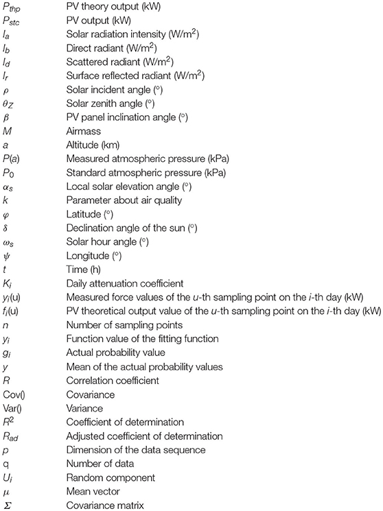
Nomenclature