CFD Simulation of Two-Phase Flows in Helical Coils

Introduction

Because of their superior heat transfer performance when compared to straight pipes and the compactness of the cylindrical geometry, helical coils are widely used in the food industry, steam generators, chemical processing, and medical equipment (Fsadni et al., 2016). In the field of nuclear engineering, helical coil designs have also been widely used for steam generators in several types of nuclear power plants such as the Otto Hahn nuclear ship reactor, the Thorium High Temperature Reactor (THTR-300), the Super Phoenix fast reactor, the Advanced Gas-cooled Reactor (AGR), the Fort St. Vrain High Temperature Gas Reactor (HTGR) and the Monju reactor (Matsuura et al., 2007; Santini et al., 2008). In addition, helical coil steam generators are considered for future reactor designs such as International Reactor Innovative and Secure (IRIS), BREST-OD-300, System-integrated Modular Advanced ReacTor (SMART), CAREM-25 and NuScale (Carelli et al., 2004; Dragunov et al., 2012; Kim et al., 2013; Marcel et al., 2013; Ingersoll et al., 2014).

El-Genk and Schriener (2017) published a literature review on convection heat transfer and pressure losses for single-phase flows in toroidal and helically coiled tubes. They collected 2,410 pressure losses data and 193 Nusselt number data and summarized the effect of the dimensions, geometric parameters, flowrates, and the fluids' properties on the critical Reynolds number, friction factor, and Nusselt number. However, in many helical coil steam generator designs, the two-phase flow appears within the coils instead of the shell side. Therefore, detailed information on pressure drops, void fraction distributions and flow regime in helical coil geometries are relevant as well. Experiments on two-phase flow in vertical helical coils have been performed in the past (Kasturi and Stepanek, 1972; Xin et al., 1996; Mandal and Das, 2003; Zhu et al., 2017) to investigate pressure losses, void fraction and flow regimes and corresponding empirical correlations have been proposed.

In the past decades, more advanced measurement techniques have been introduced that are able to provide higher resolution experimental data on void fraction distributions (Rahman et al., 2009). Experimental data from high-speed cameras, high-speed X-ray radiography, and wire-mesh sensor can provide the additional resolution for a more extensive validation of CFD models. Because of the wide range of void fraction, an interface-capturing method is the most suitable for the corresponding CFD simulations. Hirt and Nichols (1981) proposed the Volume of Fluid (VOF) approach to track and locate the free surface of immiscible phases. Previous studies have shown that this model has the capability to correctly capture void fraction distributions (Hernandez Perez, 2008; Fernandes et al., 2009; Abdulkadir, 2011; Akhlaghi et al., 2019; Kiran et al., 2020). All of them performed mesh independence studies based on a reference case, but not all showed a good agreement with the experimental data in terms of the two-phase pressure drops when the optimal mesh was extrapolated to other cases. Alizadehdakhel et al. (2009) showed that their mesh is suitable for several flow regimes with the relative error below 10 percent when compared with experimental data. In two other studies instead a large discrepancy was found when simulating flow regimes different from the reference case used to perform the mesh convergence study (Akhlaghi et al., 2019; Kiran et al., 2020). Therefore, a point of interest for the current paper is to investigate how far the extrapolation can be applied when simulating two phase flows in helical coils.

However, most of the past studies mentioned above focused on straight pipes or curved pipes and very few studies were dedicated to the simulation of two-phase flow in helical coils using VOF. In the present study, CFD simulations have been carried out using the commercial code STAR-CCM+ v13.06 and 14.04 to model air-water flows in the helical coil geometry. The simulation results are compared with the experimental data obtained by Breitenmoser et al. (2019).

Experimental Setup

The scheme of the Michigan Adiabatic Helical Coil (MAHICan) facility is reported in Figure 1. The geometrical details of the test section are summarized in Table 1. Two pressure drop transducers are used to measure the pressure drop across the entire coil and across the last half turn of the coil, upstream of the test section outlet (indicated as DP1 and DP2 in Figure 1, respectively). In addition, a high-speed X-ray radiography system was used to measure the void fraction. The X-ray measurements were performed 4.86 m, i.e., 1.5 turns downstream of the helical coil pipe entrance to avoid entrance effects. In total 136 measurements were performed for an adiabatic air-water two-phase flow in the MAHICan facility. The superficial air and water velocities for the data points range from 0.18 to 35.32 m/s and from 0.05 to 1.83 m/s, respectively. The experimental flow regime identification was based solely on the X-ray radiography measurements and the resulting postprocessed quantitative void fraction data. According to the methodology introduced by Zhu et al. (2017), the 136 measurements were classified into six different flow regimes, namely bubbly, plug, slug, wavy, slug-annular, and annular flow. More detailed information of the facility and experimental procedures are reported by Zhuang et al. (2018) and Breitenmoser et al. (2019). In the present study, 12 experimental measurements were selected as references for the CFD simulations.

FIGURE 1

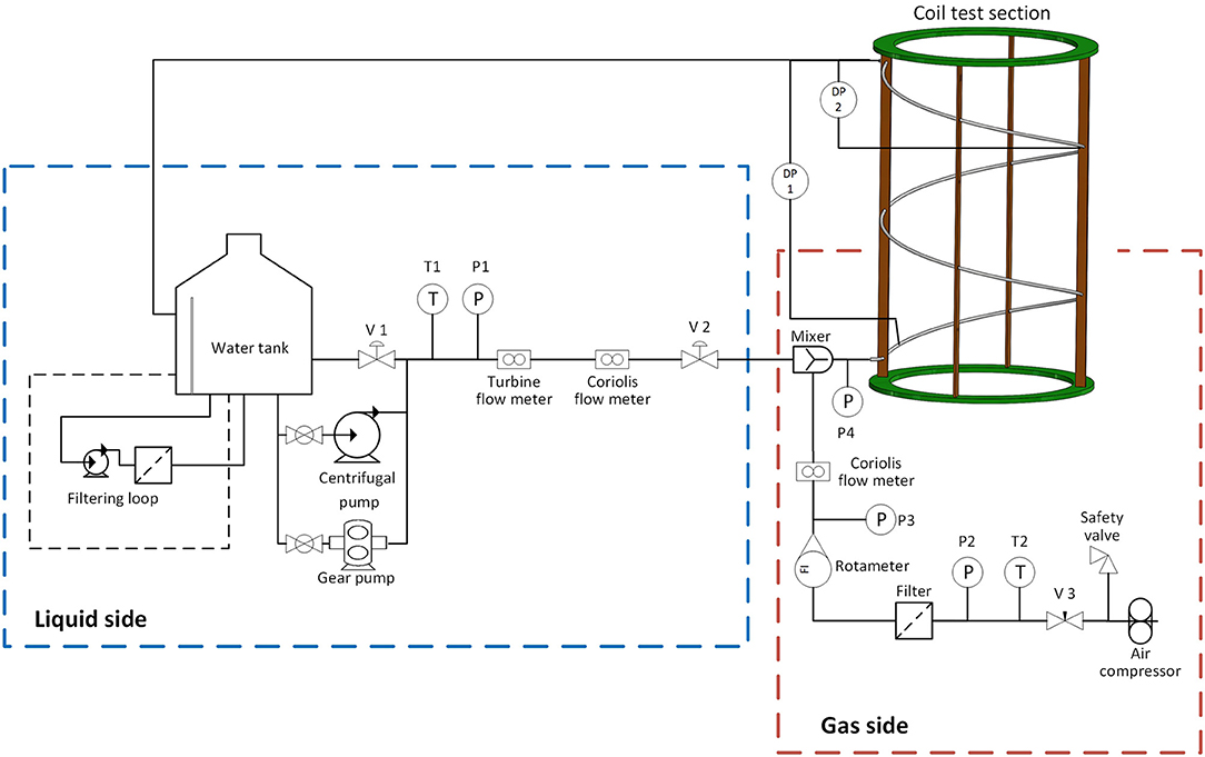
Figure 1. Scheme of the experimental facility.

TABLE 1

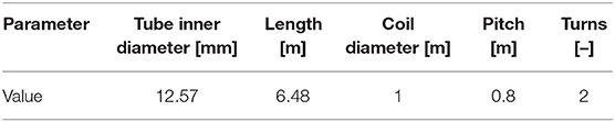
Table 1. Geometric parameters of the helical coil.

CFD Modeling

This section introduces all of the physical models used in the simulations presented below, including the multiphase flow model, multiphase interaction model, turbulence model, and transient model. Moreover, boundary and initial conditions are discussed as well.

Multiphase Flow Model

Based on the Eulerian framework, the VOF methodology was developed as an interface capturing model to predict the distribution and the movement of the interface of immiscible phases. The volume fraction of each phase in the computation domain is used to describe the distribution of phases and the position of the interface. The volume fraction of phase q is defined as:

$\begin{array}{ll}{\alpha }_q=\frac{V_q}{V}& (1)\end{array}$

where V_q is the volume of phase q in the cell and V is the volume of the cell.

The VOF model uses a single set of equations to model the multiphase flow and treats the immiscible phases as a mixture. Accordingly, the density and dynamic viscosity of the mixture are defined as the sum of volume fraction weighted properties of each phase:

$\begin{array}{ll}{\rho }_m={\displaystyle {\sum }_q}{\rho }_q{\alpha }_q& (2)\end{array}$

$\begin{array}{ll}{\mu }_m={\displaystyle {\sum }_q}{\mu }_q{\alpha }_q& (3)\end{array}$

The volume fraction transport equation is used to resolve the movement of the interface:

$\begin{array}{ll}\frac{\partial {\alpha }_q}{\partial t}+\frac{\partial ({\alpha }_q{u}_j)}{\partial x_j}+\frac{\partial }{\partial x_j}\left[C_{\alpha }|\text{u}|\frac{1}{|\nabla {\alpha }_q|}\frac{\partial {\alpha }_q}{\partial x_j}{\alpha }_q(1-{\alpha }_q)\right]=0& (4)\end{array}$

where C_α is a sharpening factor and u is the mixture velocity vector. The u_j and x_j denote, respectively, the mixture velocity component and the coordinate in the j direction, and t represents the time. The first and second term on the left hand side denote the change rate of volume fractions and convective term respectively. The third term on the left hand side is caused by the non-zero sharpening factor. The sharpening factor is used to reduce numerical diffusion in the simulation. In the present study, the sharpening factor was assigned as 1 to avoid smearing of the interface due to numerical diffusion.

The conservation equations of mixture mass and momentum are defined as follow:

$\begin{array}{ll}\frac{\partial {\rho }_m}{\partial t}+\frac{\partial ({\rho }_m{u}_j)}{\partial x_j}=0& (5)\end{array}$

$\begin{array}{l}\frac{\partial ({\rho }_m{u}_i)}{\partial t}+\frac{\partial \left({\rho }_m{u}_i{u}_j\right)}{\partial x_j}=-\frac{\partial p}{\partial x_i}+\frac{\partial }{\partial x_j}\\ \left[{\mu }_m\left(\frac{\partial u_i}{\partial x_j}+\frac{\partial u_j}{\partial x_i}\right)\right]+{\rho }_m{g}_i& (6)\end{array}$

where p and g are the mixture pressure and the gravitational acceleration respectively. The energy equation is omitted in the simulations since the experiments were carried out in adiabatic conditions.

The accuracy of the VOF model depends on the mesh grid or cell size. At least three cells across each bubble are required to fully capture the interface between two phases (Siemens, 2018). As a result, this model is computationally suitable for simulating flows in which large two-phase structures are present.

Moreover, the multiphase interaction model is crucial for the interface reconstruction that directly determines the accuracy of the void fraction distribution. Taha and Cui (2006) performed numerical simulations to study the motion of single Taylor bubbles in vertical tubes. They concluded that the terminal rising velocity and shape of slug in air-water flows are significantly affected by surface tension and buoyancy force. Surface tension is particularly important for multiphase flows in the presence of strongly curved surfaces. In the VOF model, the surface tension is introduced as a body force by adding a momentum term to the momentum equation. In STAR CCM+, the interfacial surface force is modeled as a volumetric force using the Continuum Surface Force (CSF) approach proposed by Brackbill et al. (1992). Therefore, this model was selected and a constant surface tension of 0.072 N/m was specified in the present study, corresponding to the surface tension of water-air at the operating temperature of 20°C. In addition, for the VOF-VOF phase interaction model, the water was selected as the primary phase.

Turbulence Model

To model the turbulence in multiphase flows, the k-ϵ model is recommended for internal flows and the k-ω model for external flows (Siemens, 2018). The standard k-ϵ model requires the solution of two transport equations for the turbulence kinetic energy (k) and the turbulence dissipation rate (ϵ) respectively:

$\begin{array}{ll}\frac{\partial k}{\partial t}+u_j\frac{\partial k}{\partial x_j}={\tau }_{Rij}\frac{\partial u_i}{\partial x_j}-ϵ+\frac{\partial }{\partial x_j}\left[\left(\nu +\frac{{\nu }_t}{{\sigma }_k}\right)\frac{\partial k}{\partial x_j}\right]& (7)\end{array}$

$\begin{array}{ll}\frac{\partial ϵ}{\partial t}+u_j\frac{\partial ϵ}{\partial x_j}=C_{ϵ1}\frac{ϵ}{k}{\tau }_{Rij}\frac{\partial u_i}{\partial x_j}-C_{ϵ2}\frac{{ϵ}^2}{k}+\frac{\partial }{\partial x_j}\left[(\nu +\frac{{\nu }_t}{{\sigma }_{ϵ}})\frac{\partial ϵ}{\partial x_j}\right]& (8)\end{array}$

where the τ_Rij is the Reynolds stress tensor, ν is the kinematic viscosity, ν_t is the turbulence eddy viscosity, and C_ϵ1, C_ϵ2, σ_ϵ, σ_k are model coefficients. This model is based on the eddy viscosity approximation to relate the Reynolds stress tensor to the local mean flow strain rate tensor $\overline{S_{ij}}$:

$\begin{array}{ll}{\tau }_{Rij}=-\overline{u_i\prime u_j\prime }=2{\nu }_t{\overline{S}}_{ij}-\frac{2}{3}k{\delta }_{ij}& (9)\end{array}$

$\begin{array}{ll}{\nu }_t=C_{\mu }\frac{k^2}{ϵ}& (10)\end{array}$

where $u_i\prime$ and $u_j\prime$ is the velocity fluctuation component in i and j direction, δ_ij is the delta function, and C_μ is a model coefficient.

For the realizable k-ϵ model, the equation for the turbulent dissipation rate is modified, and the model coefficient C_μ is expressed as a function of mean flow and turbulence properties instead of a constant. These two modifications to the formulation of the standard k-ϵ model guarantees that mathematical requirements (positive normal Reynold stresses and Schwartz inequality) based on the physics of turbulence are always satisfied. Hence, the realizable k-ϵ model was selected for the simulation of internal flows in the helical coil.

Owing to the unsteady nature of the two-phase flow, the simulations were performed in transient mode and the implicit unsteady numerical scheme was selected. The integration time-step convergence study is discussed in section mesh generation and convergence study. All simulations were run for 4 s of transient time.

Boundary and Initial Conditions

In the present study, only the coil test section shown in Figure 1 was simulated. The dimensions of the helical coil are reported in Table 1. A mixer installed upstream of the test section inlet provides a uniform two-phase mixture at the inlet of the test section. Detailed information on the mixer geometry was reported by Zhuang et al. (2018). A pressure transducer was installed to measure the mixture pressure, together with two pressure drop sensors, as discussed in section experimental setup. The properties of air and water were specified based on the measured mixture pressure and temperature. The results of the simulations in the present study show that the air density, as well as the water density, plays a minor role, therefore, the constant density model was applied for both air and water in the finalized CFD simulations.

The inlet and outlet boundaries of the helical coil were defined as a “velocity inlet” and “outlet” boundary conditions respectively. The mixture velocity and void fraction were specified at the inlet, based on the measured experimental data. For the coil pipe walls, a no-slip wall condition was imposed. Due to the large range of wall y⁺ value induced by different properties of air and water, the two-layer all y⁺ wall treatment was used. The surface average wall y⁺ values obtained in the simulations range from 23.6 to 106.2, indicating that the mesh wall discretization is appropriate for the turbulence model. For the simulations initial condition, the computational domain was specified as stagnant water to ease the convergence process.

Mesh Generation and Convergence Study

Before performing the CFD simulations, a convergence study was carried out to guarantee the computational solution is not affected by the selected mesh size and integration time step. The reference case selected for the convergence study corresponds to inlet gas and liquid superficial velocities of 2.85 and 1.5 m/s respectively (cf. Table 2), i.e., the test No. 7.

TABLE 2

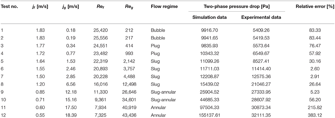
Table 2. Comparison between experimental and CFD-predicted pressure drops.

Mesh Convergence Study

The most suitable mesh type for two-phase flows in the pipe geometry is given by the O-grid mesh (Hernandez-Perez et al., 2011), so this type of mesh was selected for the present study. Firstly a surface O-grid mesh is generated on the inlet surface and then it is extruded equally along the axis of the helical coil as shown in Figure 2.

FIGURE 2

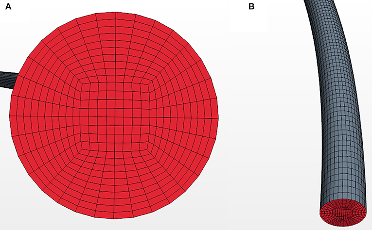
Figure 2. O-grid mesh (A) on the initial cross section and (B) in axial direction.

The prism layer is uniformly generated from the wall, and defined by 10 equal spacing nodes. The growth factor of the prism layer is 1 and the thickness of each cell is around 0.35 mm. In the center of the cross section, the side length of one square shape cell is about 0.5 mm, which is small enough to capture the large structure of free surface like Taylor bubbles in the helical coil when compared with the diameter of the coil, 12.57 mm. Therefore, seven simulations were performed to investigate the effect of the number of axial layers. The nodalization along the axis of the helical coil was changed from 1.62 mm (corresponding to 4,000 axial layers) to 6.48 mm (corresponding to 1,000 axial layers).

The results of the two-phase pressure drop for the last half turn upstream of the helical coil outlet and the void fraction at 1.5 turns downstream of the coil inlet are shown in Figure 3. The two-phase pressure drop is averaged from the time that the first bubble goes through the outlet to the end of simulation, and the time-averaged void fraction is evaluated from 2 to 4 s. The dashed lines in Figure 3 represent the experimental data. It is clear that increasing the number of axial layer makes the results close to the experimental data. A large variation occurs refining the mesh from 1,000 to 2,000 axial layers. The relative differences between the intermediate mesh (3,000 layers) and the finest mesh (4,000 layers) are <3 and 0.7% for pressure drop and void fraction, respectively. Therefore, an axial mesh consisting of 3,000 axial layers was selected for the simulations reported in section results and discussion.

FIGURE 3

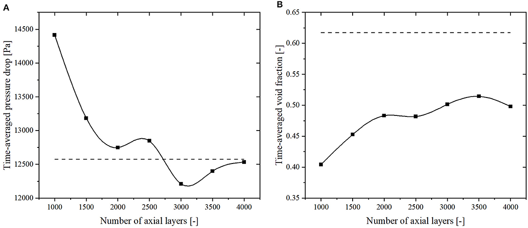
Figure 3. Results of the mesh convergence study. (A) Two-phase pressure drop. (B) Void fraction.

Time Step Convergence Study

Four simulations were performed using different integration time steps ranging from 0.05 ms up to 0.5 ms, and the results of the time dependent void fraction averaged over a selected volume of the helical coil are shown in Figure 5. The dimensions and location of the volume on which the void fraction has been averaged is the same used by Breitenmoser et al. (2019) to postprocess the experimental data.

In the test No. 7, the slug flow regime occurs as indicated by the experimental data. The time step convergence study shows that if the integration time step is larger than 0.1 ms, the simulation is not able to capture the characteristic of slug flow, as demonstrated in Figures 4A,B. In contrast, simulations with a smaller time step show a good agreement with the experimental data as indicated in Figure 9A. In Figures 4C,D, the repeating high peaks represent the large slug bubbles passing through the volume selected for the void fraction spatial averaging, and the fluctuations after the peaks correspond to the wake behind a large slug bubble.

FIGURE 4

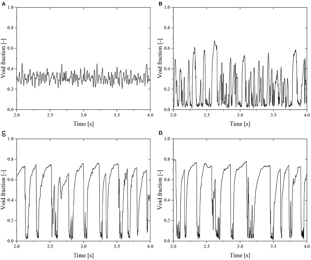
Figure 4. Simulation data of void fraction for different integration time steps. (A) Time-step = 0.5 ms. (B) Time-step = 0.2 ms. (C) Time-step = 0.1 ms. (D) Time-step = 0.05 ms.

In addition, the time-averaged data was also investigated as shown in Figure 5, and the same time-averaged range as mentioned in previous subsection was used. There is a clear convergence trend from 0.5 to 0.1 ms and the experimental data is indicated by the dashed lines. The relative differences between the smallest time step (0.05 ms) and the intermediate time step (0.1 ms) are <1.5% for both parameters. To reduce the computational time associated to the simulations, a time step of 0.1 ms was selected for the results discussed in section results and discussion.

FIGURE 5

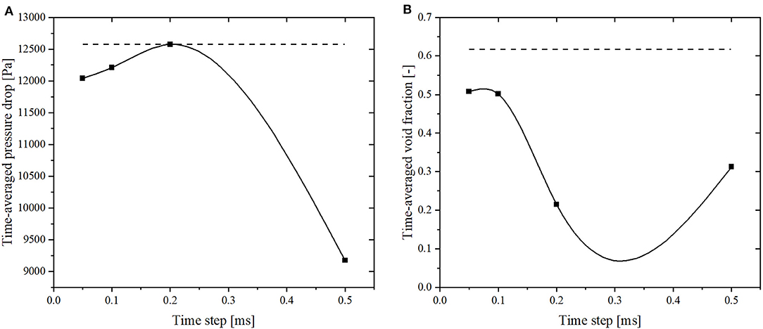
Figure 5. Results of the time step convergence study. (A) Two-phase pressure drop. (B) Void fraction.

Results and Discussion

In this section, the simulation results for two-phase pressure drops and time-dependent volume averaged void fractions are presented and compared with the experimental data. All of the following figures are obtained using Origin Pro 2019.

Two-Phase Pressure Drop

As mentioned earlier, the two-phase pressure drop is an important parameter for designing a new helical coil heat exchanger. In the experiments, the two-phase pressure drops for the last half turn upstream of the helical coil outlet were measured, so in the simulations, the pressure drop across the same section was monitored for comparison with the experimental data. The comparison obtained for the time-averaged pressure drop is reported in Table 2.

The results show that for the slug and slug-annular flow regimes (tests No. 5 to No. 9), the two-phase pressure drops can be predicted reasonably well with relative errors ranging from <3% to up to about 30%. This also supports the conclusion that the VOF model is suitable for modeling immiscible two-phase flows in which large structures are present. However, for all other flow regimes, the two-phase pressures drops are all significantly overestimated with relative errors up to more than 300%.

The possible reason for the poor agreement between the simulation and experiment could be explained by the fact that the superficial velocities and flow patterns of the other cases are far from the reference case No. 7 for which the mesh and time-step convergence study were performed. There are few other cases (test No. 5, No. 6, No. 8, and No. 9) which shows reasonable agreement with experimental data and also has reasonably similar close superficial velocities and belongs to the same flow regime. However, the large discrepancy in results between simulations and experimental data suggests that mesh and time-step should be verified on a case-specific basis and cannot be extrapolated too far from the reference case. With this, we can conclude that universal mesh and time-step for this modeling approach does not exist due to significant variation in boundary conditions imposed for different cases. The possible reasons for the poor agreement for each flow regime are presented in the next subsection with the analysis of the void fraction distribution.

Void Fraction

In this subsection, the results of the void fraction are compared between the experimental and CFD-predicted data. All of 12 tests are separated into five different flow regimes, and six representative results for the different identified flow regimes are presented and discussed.

Bubbly Flow

The test No. 1 and No. 2 correspond to the bubbly flow regime. The time evolution of the void fraction and the corresponding void fraction histogram of test No. 2 for both experimental and simulation data are shown in Figure 6. The void fraction time evolution in Figure 6A shows small oscillations around 0.02 and the maximum void fraction is <0.1. However, the simulation results in Figure 6B show much larger peaks and more frequent oscillations, which means that the simulation produces larger bubbles which move faster than in the experiment. Figures 6E,F confirm that the computational model results in larger bubbles than what found in the experiments. This might be due to the mesh not being fine enough to capture the small bubbles, which leads to small bubbles merged into a large bubble. As mentioned above, in subsection multiphase flow model, at least three cells across a small bubble are required to capture the interface between two immiscible phases fully. It is evident that the finer mesh helps simulate smaller bubbles better, but the simulations will become too expensive to afford. Nevertheless, both the two histograms reported in Figures 6C,D demonstrate a unimodal void fraction distribution peaked at low void fraction values, caused by the dominant continuous liquid phase present in bubbly flow. Due to the low void fraction, i.e., high X-ray attenuation, the noise level in the experimental data is relatively high compared to other flow regimes. This noise causes some values of the measured void fraction to be <0, as demonstrated in Figure 6A.

FIGURE 6

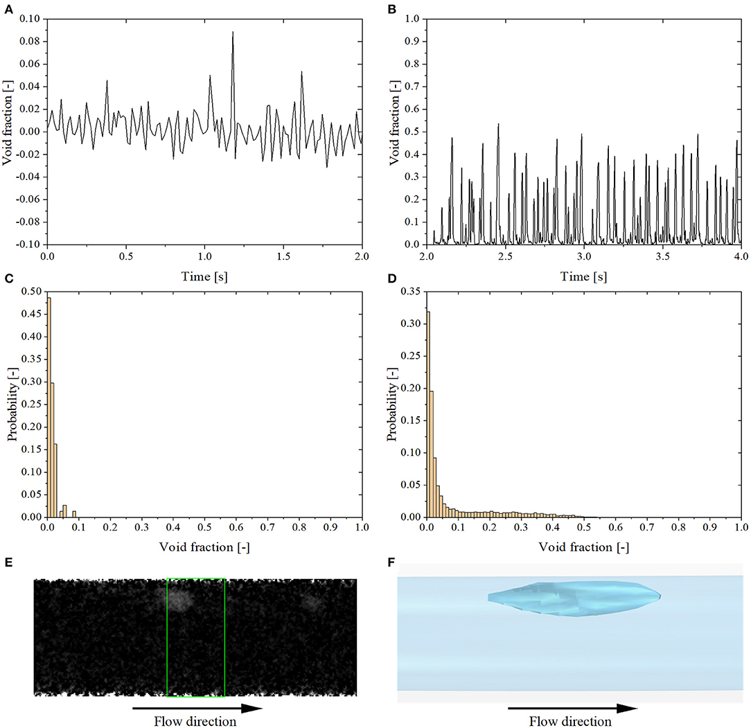
Figure 6. Results of test No. 2. (A) Experimental void fraction time evolution. (B) Simulation void fraction time evolution. (C) Experimental void fraction histogram. (D) Simulation void fraction histogram. (E) X-ray void fraction contrast image. (F) Void fraction isosurface image.

Plug Flow

By increasing the air flow rate, the small bubbles tend to agglomerate together and the bubble clusters develop into elongated Taylor bubbles or plugs. According to the definition of Zhu et al. (2017), tests No. 3 and No. 4 are identified as plug flow regime. As shown in Figures 7A,B, the peaks values are similar for the simulation and experiments, but still the simulation shows the occurrence of peaks at higher frequency than the experimental data. In terms of the histograms, the void fraction histogram presents a bimodal distribution with the appearance of a second peak in the high void fraction range, around 0.5 (cf. Figures 7C,D). Since the plug flow is characterized by large structures, the simulation is able to correctly capture the phenomenology observed in the experiments (cf. Figures 7E,F). In addition, the staircase shaped tail of a plug proposed by Conte et al. (2017) can be seen both in Figures 7E,F. However, the mesh used in these two simulations is still not fine enough to track the interfaces of small bubbles, which might lead to the large discrepancy for the two-phase pressure drop.

FIGURE 7

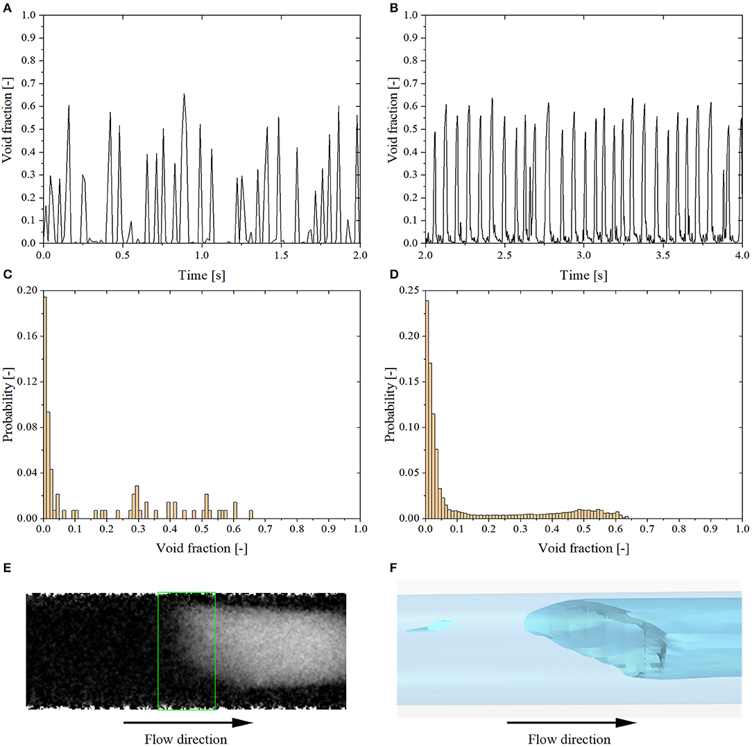
Figure 7. Results of test No. 3. (A) Experimental void fraction time evolution. (B) Simulation void fraction time evolution. (C) Experimental void fraction histogram. (D) Simulation void fraction histogram. (E) X-ray void fraction contrast image. (F) Void fraction isosurface image.

Slug Flow

With higher air superficial velocity, the flow regime transits from plug to slug flow. This flow regime is characterized by higher and wider void fraction peaks, as illustrated in Figures 8, 9. However, in the simulation, the Taylor bubbles are longer than in experiments and have lower peak values of void fraction compared with the experimental data (cf. Figures 8A,B, 9A,B). The slug flow regime is identified for tests No. 5 to No. 8 (cf. Table 2). In addition, the second void fraction peak in the histogram becomes higher than the first peak as shown in Figures 8C,D, 9C,D. Besides, as shown in Figures 9E,F, a slug tail similar to what observed in the experiments is predicted in the simulation.

FIGURE 8

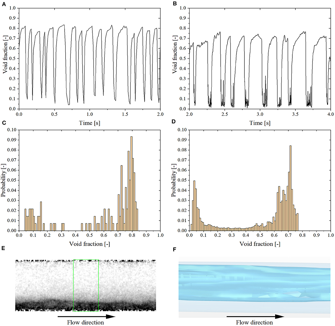
Figure 8. Results of test No. 6. (A) Experimental void fraction time evolution. (B) Simulation void fraction time evolution. (C) Experimental void fraction histogram. (D) Simulation void fraction histogram. (E) X-ray void fraction contrast image. (F) Void fraction isosurface image.

FIGURE 9

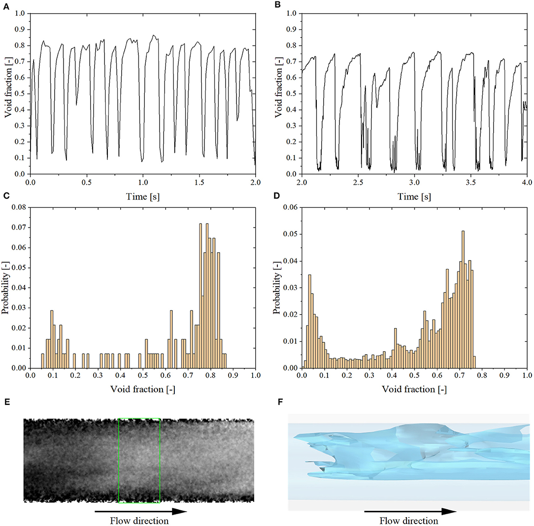
Figure 9. Results of test No. 7. (A) Experimental void fraction time evolution. (B) Simulation void fraction time evolution. (C) Experimental void fraction histogram. (D) Simulation void fraction histogram. (E) X-ray void fraction contrast image. (F) Void fraction isosurface image.

Slug-Annular Flow

Based on the definition proposed by Zhu et al. (2017), tests No. 9 and No. 10 are identified as slug-annular flow regime. Due to the higher air superficial velocity, some of the long Taylor bubbles coalesce together, showing typical features of annular flow. In Figure 10F, cavities on the slug bubble surface induced by the high air superficial velocity are clearly visible, while they are hard to notice from a 2d projection in Figure 10E. As a result, the number of large oscillations decreases and the void fraction fluctuates around 0.8 (cf. Figures 10A,B). The void fraction histogram return to a unimodal distribution, but with the peak located at higher void fraction values (cf. Figures 10C,D). As shown in Table 2, the air superficial velocity of test No. 10 is five-time larger than the reference case (test No. 7), so the large discrepancy between experiments and simulations is probably due to a not sufficiently small integration time step.

FIGURE 10

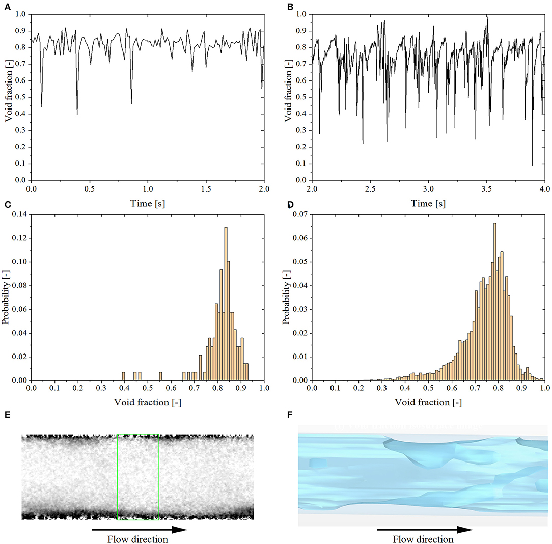
Figure 10. Results of test No. 9. (A) Experimental void fraction time evolution. (B) Simulation void fraction time evolution. (C) Experimental void fraction histogram. (D) Simulation void fraction histogram. (E) X-ray void fraction contrast image. (F) Void fraction isosurface image.

Annular Flow

Tests No. 11 and No. 12 correspond to the annular flow regime. The main characteristic of the transition from slug-annular flow to annular flow is the disappearance of the slugs. The smooth annular region appears both in the experiment and simulation (cf. Figures 11E,F). Therefore, there is a unimodal void fraction distribution present in the histogram with a single peak in the high void fraction regime (cf. Figures 11C,D). Comparing with the experimental data, the simulation results still show some slugs, not found in the experimental data (cf. Figures 11A,B). This might explain why the computed two-phase pressure drops are much larger than the experimental data (cf. Table 2). Another possible reason of the large difference is that the annular flow simulation requires smaller time step owing to the highest air superficial velocity. The time step convergence used test No. 7 as a reference and it was extrapolated into other 11 simulations, so the time step may not be accurate enough. The smaller time step might give better results, but it absolutely makes the computation much more expensive.

FIGURE 11

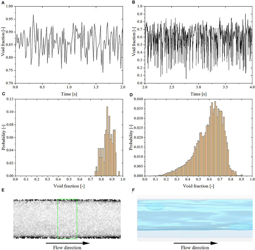
Figure 11. Results of test No. 11. (A) Experimental void fraction time evolution. (B) Simulation void fraction time evolution. (C) Experimental void fraction histogram. (D) Simulation void fraction histogram. (E) X-ray void fraction contrast image. (F) Void fraction isosurface image.

Conclusion

The behavior of air-water two-phase adiabatic flows in helical coils was investigated using CFD simulations. The VOF model was applied to track and locate the free surface of two immiscible phases, namely water and air. The realizable k-ϵ model was employed to simulate the turbulence of the two-phase flow. Following a convergence study, the optimal parameters for mesh generation and integration time steps were determined based on the reference case, test No. 7. The simulation results show that by employing proper boundary conditions, initial conditions, mesh and time step, the air-water flow regime as well as the pressure drop can be predicted by CFD models reasonably well. The bubbly, plug, slug, slug-annular and annular flow regimes were observed in the simulations, but a good quantitative agreement with the experimental data for two-phase pressure drops and void fractions was found only for slug and slug-annular flow regimes. This good quantitative agreement proves that the VOF model can predict and capture the two-phase flow very well with the case-specific mesh and time-step convergence study. However, for other cases, the two-phase pressure drops were considerably overestimated in the simulations, and phenomenological differences for the void fraction time evolutions were also observed. The large discrepancy of pressure drops and time-dependent void fraction shown in these cases confirms that the optimal mesh and time-step obtained for the reference case cannot be used for different flow regimes cases, especially for those whose superficial velocities differ a lot from the reference case. Also, there is not a single mesh that can be used to simulate all the flow regimes due to the significant flow topology variation. Hence, a case-specific mesh and time-step convergency are indispensable for each flow regime.

Data Availability Statement

The datasets generated for this study are available on request to the corresponding author.

Author Contributions

SC is the main author of the paper and was responsible for drafting the paper and performing the numerical simulations. DB carried out the experiments, the associated experimental data post-processing and provided the experimental data. YI, AM, and VP are the group supervisors and have provided SC and DB with technical guidance on the execution of the computational and experimental work and on the drafting of this manuscript.

Funding

This work was partially funded by a DOE NEAMS HIP grant and by the China Scholarship Council.

Conflict of Interest

The authors declare that the research was conducted in the absence of any commercial or financial relationships that could be construed as a potential conflict of interest.

Acknowledgments

The work presented herein was supported by the US Department of Energy's Nuclear Energy Advanced Modeling and Simulation (NEAMS) program as part of the Steam Generator Flow Induced Vibration High Impact Problem, by the China Scholarship Council, and by the Advanced Research Computing at the University of Michigan, Ann Arbor.

References

Abdulkadir, M. (2011). Experimental and Computational Fluid Dynamics (CFD) studies of gas-liquid flow in bends. (Ph.D. thesis). Nottingham, UK: University of Nottingham.

Google Scholar

Akhlaghi, M., Mohammadi, V., Nouri, N. M., Taherkhani, M., and Karimi, M. (2019). Multi-fluid VoF model assessment to simulate the horizontal air–water intermittent flow. Chem. Eng. Res. Des. 152, 48–59. doi: 10.1016/j.cherd.2019.09.031

CrossRef Full Text | Google Scholar

Alizadehdakhel, A., Rahimi, M., Sanjari, J., and Alsairafi, A. A. (2009). CFD and artificial neural network modeling of two-phase flow pressure drop. Int. Commun. Heat Mass Transf. 36, 850–856. doi: 10.1016/j.icheatmasstransfer.2009.05.005

CrossRef Full Text | Google Scholar

Brackbill, J. U., Kothe, D. B., and Zemach, C. (1992). A continuum method for modeling surface tension. J. Comput. Phys. 100, 335–354. doi: 10.1016/0021-9991(92)90240-Y

CrossRef Full Text | Google Scholar

Breitenmoser, D., Manera, A., Prasser, H. M., and Petrov, V. (2019). “High-resolution high-speed void fraction measurements in helical tubes using X-ray radiography,” in 18th International Topical Meeting on Nuclear Reactor Thermal Hydraulics (NURETH 2019) (Portland), 3554–3567.

Google Scholar

Carelli, M. D., Conway, L. E., Oriani, L., Petrovic, B., Lombardi, C., Ricotti, M. E., et al. (2004). The design and safety features of the IRIS reactor. Nuclear Eng. Des. 230, 151–167. doi: 10.1016/j.nucengdes.2003.11.022

CrossRef Full Text | Google Scholar

Conte, M. G., Hegde, G. A., da Silva, M. J., Sum, A. K., and Morales, R. E. M. (2017). Characterization of slug initiation for horizontal air-water two-phase flow. Exp. Therm. Fluid Sci. 87, 80–92. doi: 10.1016/j.expthermflusci.2017.04.023

CrossRef Full Text | Google Scholar

Dragunov, Y. G., Lemekhov, V. V., Smirnov, V. S., and Chernetsov, N. G. (2012). Technical solutions and development stages for the BREST-OD-300 reactor unit. Atomic Energy 113, 70–77. doi: 10.1007/s10512-012-9597-3

CrossRef Full Text | Google Scholar

El-Genk, M. S., and Schriener, T. M. (2017). A review and correlations for convection heat transfer and pressure losses in toroidal and helically coiled tubes. Heat Transf. Eng. 38, 447–474. doi: 10.1080/01457632.2016.1194693

CrossRef Full Text | Google Scholar

Fernandes, J., Lisboa, P. F., Simoes, P. C., Mota, J. P. B., and Saatdjian, E. (2009). Application of CFD in the study of supercritical fluid extraction with structured packing: wet pressure drop calculations. J. Supercrit. Fluids 50, 61–68. doi: 10.1016/j.supflu.2009.04.009

CrossRef Full Text | Google Scholar

Fsadni, A. M., Whitty, J. P., and Stables, M. A. (2016). A brief review on frictional pressure drop reduction studies for laminar and turbulent flow in helically coiled tubes. Appl. Therm. Eng. 109, 334–343. doi: 10.1016/j.applthermaleng.2016.08.068

CrossRef Full Text | Google Scholar

Hernandez Perez, V. (2008). Gas-liquid two-phase flow in inclined pipes. (Ph.D. thesis). Nottingham, UK: University of Nottingham.

Google Scholar

Hernandez-Perez, V., Abdulkadir, M., and Azzopardi, B. (2011). Grid generation issues in the CFD modelling of two-phase flow in a pipe. J. Comput. Multiphase Flows 3, 13–26. doi: 10.1260/1757-482X.3.1.13

CrossRef Full Text | Google Scholar

Hirt, C. W., and Nichols, B. D. (1981). Volume of Fluid (Vof) method for the dynamics of free boundaries. J. Comput. Phys. 39, 201–225. doi: 10.1016/0021-9991(81)90145-5

CrossRef Full Text | Google Scholar

Ingersoll, D. T., Houghton, Z. J., Bromm, R., and Desportes, C. (2014). NuScale small modular reactor for Co-generation of electricity and water. Desalination 340, 84–93. doi: 10.1016/j.desal.2014.02.023

CrossRef Full Text | Google Scholar

Kasturi, G., and Stepanek, J. (1972). Two phase flow—I. pressure drop and void fraction measurements in concurrent gas-liquid flow in a coil. Chem. Eng. Sci. 27, 1871–1880. doi: 10.1016/0009-2509(72)85049-8

CrossRef Full Text | Google Scholar

Kim, H. K., Kim, S. H., Chung, Y. J., and Kim, H. S. (2013). Thermal-hydraulic analysis of SMART steam generator tube rupture using TASS/SMR-S code. Ann. Nuclear Energy 55, 331–340. doi: 10.1016/j.anucene.2013.01.007

CrossRef Full Text | Google Scholar

Kiran, R., Ahmed, R., and Salehi, S. (2020). Experiments and CFD modelling for two phase flow in a vertical annulus. Chem. Eng. Res. Des. 153, 201–211. doi: 10.1016/j.cherd.2019.10.012

CrossRef Full Text | Google Scholar

Mandal, S. N., and Das, S. K. (2003). Gas–liquid flow through helical coils in vertical orientation. Ind. Eng. Chem. Res. 42, 3487–3494. doi: 10.1021/ie0200656

CrossRef Full Text | Google Scholar

Marcel, C. P., Acuna, F. M., Zanocco, P. G., and Delmastro, D. F. (2013). Stability of self-pressurized, natural circulation, low thermo-dynamic quality, nuclear reactors: the stability performance of the CAREM-25 reactor. Nuclear Eng. Des. 265, 232–243. doi: 10.1016/j.nucengdes.2013.08.057

CrossRef Full Text | Google Scholar

Matsuura, M., Hatori, M., and Ikeda, M. (2007). Design and modification of steam generator safety system of FBR MONJU. Nuclear Eng. Des. 237, 1419–1428. doi: 10.1016/j.nucengdes.2006.09.046

CrossRef Full Text | Google Scholar

Rahman, M., Heidrick, T., and Fleck, B. (2009). A critical review of advanced experimental techniques to measure two-phase gas/liquid flow. Open Fuels Energy Sci. J. 2, 54–70. doi: 10.2174/1876973X00902010054

CrossRef Full Text | Google Scholar

Santini, L., Cioncolini, A., Lombardi, C., and Ricotti, M. (2008). Two-phase pressure drops in a helically coiled steam generator. Int. J. Heat Mass Transf. 51, 4926–4939. doi: 10.1016/j.ijheatmasstransfer.2008.02.034

CrossRef Full Text | Google Scholar

Siemens, P. (2018). Simcenter STAR-CCM+ User Guide V13. 06. Plano: Siemens PLM.

Google Scholar

Taha, T., and Cui, Z. F. (2006). CFD modelling of slug flow in vertical tubes. Chem. Eng. Sci. 61, 676–687. doi: 10.1016/j.ces.2005.07.022

CrossRef Full Text | Google Scholar

Xin, R. C., Awwad, A., Dong, Z. F., Ebadian, M. A., and Soliman, H. M. (1996). An investigation and comparative study of the pressure drop in air-water two-phase flow in vertical helicoidal pipes. Int. J. Heat Mass Transf. 39, 735–743. doi: 10.1016/0017-9310(95)00164-6

CrossRef Full Text | Google Scholar

Zhu, H. Y., Li, Z. X., Yang, X. T., Zhu, G. Y., Tu, J. Y., and Jiang, S. Y. (2017). Flow regime identification for upward two-phase flow in helically coiled tubes. Chem. Eng. J. 308, 606–618. doi: 10.1016/j.cej.2016.09.100

CrossRef Full Text | Google Scholar

Zhuang, N., Zhang, K., Manera, A., and Petrov, V. (2018). X-ray radiography and high-speed videography measurement on void fraction in helical coil. Adv. Thermal Hydraul. 2018, 250−262.

Google Scholar