A Stochastic Approach to the Synchronization of Coupled Oscillators

1. Introduction

Synchronization is a common phenomenon which has been observed in biological, chemical, physical and social systems for centuries and has attracted the interest of researchers in a diversified spectrum of scientific fields.

Common examples of synchronization phenomena often cited in review articles include groups of synchronously chirping crickets (Walker, 1969), fireflies flashing in unison (Buck, 1988), superconducting Josephson junction (Wiesenfeld et al., 1998), or crowds of people walking together that will tend to synchronize their footsteps (Strogatz et al., 2005).

Roughly speaking, synchronization means that a network of several periodic processes with different natural frequencies reaches an equilibrium configuration sharing the same common frequency as a result of their mutual interaction.

This concept is closely related to the one of consensus for multi-agent systems, widely analyzed in many different frameworks including collective behavior of flocks and swarms, opinion formation, and distributed computing (see Ben-Naim, 2005; Mehyar et al., 2005; Olfati-Saber, 2006; Olfati-Saber et al., 2007; Biccari et al., 2019). In broad terms, consensus means to reach an agreement regarding a certain quantity of interest that depends on the state of all agents.

Synchronization is also a key issue in power electrical engineering, for instance in the model and stability analysis of utility power grids (Sachtjen et al., 2000; Strogatz, 2001; Chassin and Posse, 2005; Filatrella et al., 2008). Indeed, large networks of connected power plants need to be synchronized to the same frequency in order to work properly and prevent the occurrence of blackouts.

Synchronization phenomena are most often characterized by the so-called Kuramoto model (Kuramoto, 1975), describing the dynamical behavior of a (large) network of oscillators in a all-to-all coupled configuration in which every oscillator is connected with all the others. This model extends the original studies by Winfree in the context of mutual synchronization in multi-oscillator systems based on a phase description (Winfree, 1967). In particular, in Kuramoto's work, synchronization appears as an asymptotic pattern which is spontaneously reached by the system when the interactions among the oscillators are sufficiently strong.

In some more recent contribution, control theoretic methods have been employed to analyze the synchronization phenomenon. For instance, in Chopra and Spong (2006) the authors design passivity-based controls for the synchronization of multi-agent systems, with application to the general problem of multi-robot coordination. In Sepulchre et al. (2005), feedback control laws for the stabilization of coupled oscillators are designed and analyzed. In Rosenblum and Pikovsky (2004) and Tukhlina et al. (2007), the authors propose methods for the suppression of synchrony in a globally coupled oscillator network, based on (possibly time-delayed) feedback schemes. Finally, Nabi and Moehlis (2011) deals with the problem of desynchronizing a network of synchronized and globally coupled neurons using an input to a single neuron. This is done in the spirit of dynamic programming, by minimizing a certain cost function over the whole state space.

In this work, we address the synchronization problem for coupled oscillators through the construction of a suitable control function via an appropriate optimization process. To this end, we propose a novel approach which combines a standard Gradient Descent (GD) methodology with the recently-developed Random Batch Method (RBM, see Jin et al., 2020) for the efficient numerical approximation of collective dynamics. This methodology has the main advantage of allowing to significantly reduce the computational complexity of the optimization process, especially when considering oscillator networks of large size, yielding to an efficient control calculation.

At this regard, we shall mention that GD methodologies have already been applied in the context of the Kuramoto model. For instance, in Taylor et al. (2016), the author develop GD algorithms to efficiently solve optimization problems that aim to maximize phase synchronization via network modifications. Moreover, in Markdahl et al. (2020), optimization and control theory techniques are applied to investigate the synchronization properties of a generalized Kuramoto model in which each oscillator lives on a compact, real Stiefel manifold. Nevertheless, to the best of our knowledge, the employment of stochastic techniques such as RBM to improve the efficiency of the GD strategy has never been proposed in the context of the Kuramoto model.

For completeness, let us stress that stochastic approaches have been widely considered, especially by the machine learning community, for treating minimization problems depending on very large data set. In this context, they have shown amazing performances in terms of the computational efficiency (see, for instance, Bottou et al., 2018 and the references therein). Nowadays, stochastic techniques are among the preeminent optimization methods in fields like empirical risk minimization (Shalev-Shwartz and Zhang, 2014), data mining (Toscher and Jahrer, 2010) or artificial neural networks (Schmidhuber, 2015).

This contribution is organized as follows: in section 2, we present the Kuramoto model and we discuss some of its more relevant properties. We also provide there a rigorous mathematical characterization of the synchronization phenomenon. In section 3, we introduce the controlled Kuramoto model and we describe the GD methodology for the control computation. Moreover, we briefly present the RBM approach and its inclusion into the GD algorithm. Section 4 is devoted to the numerical simulations and to the comparison of the two optimization techniques considered in this paper. Finally, in section 5 we summarize and discuss our results.

2. The Mathematical Model

From a mathematical viewpoint, synchronization phenomena are most often described through the so-called Kuramoto model, consisting of a population of N ≥ 2 coupled oscillators whose dynamics are governed by the following system of non-linear first-order ordinary differential equations

$\begin{array}{ll}\begin{array}{l}\{\begin{array}{l}{\dot{\theta }}_i(t)={\omega }_i+\frac{K}{N}{\displaystyle \sum _{j=1}^N\text{sin}}({\theta }_j(t)-{\theta }_i(t)),i=1,\dots ,N,t>0\hfill \\ {\theta }_i(0)={\theta }_i^0,\hfill \end{array}\hfill \end{array}& (1)\end{array}$

where θ_i(t), i = 1, …, N, is the phase of the i-th oscillator, ω_i is its natural frequency and K is the coupling strength.

The frequencies ω_i are assumed to be distributed with a given probability density f(ω), unimodal and symmetric around the mean frequency

$\begin{array}{l}\Omega =\frac{1}{N}{\displaystyle \sum _{i=1}^N}{\omega }_i,\end{array}$

that is, f(Ω + ω) = f(Ω − ω).

In this framework, each oscillator tries to run independently at its own frequency, while the coupling tends to synchronize it to all the others.

In the literature, many notions of synchronization have been considered. For identical oscillators (i.e., those in which ${\omega }_i=\hat{\omega }$ for every i = 1, …, N), one often studies whether the network can reach a configuration in which all the phases converge to the same value, that is

$\begin{array}{ll}{\displaystyle \underset{t\to +\infty }{\text{lim}}}|{\theta }_i(t)-{\theta }_j(t)|=0,\text{ for all }i,j=1,\dots ,N.& (2)\end{array}$

For systems with heterogeneous dynamics, such as when the natural frequencies ω_i are not all identical (which is typical in real-world scenarios), this definition of synchronization is too restrictive (see Sun et al., 2009). In these cases, Equation (2) is replaced by the alignment condition

$\begin{array}{ll}\begin{array}{c}\underset{t\to +\infty }{\text{lim}}|{\dot{\theta }}_i(t)-{\dot{\theta }}_j(t)|=0,\text{ for all }i,j=1,\dots ,N,\end{array}& (3)\end{array}$

according to which synchronization occurs when the phase differences given by |θ_i(t)−θ_j(t)| become constant asymptotically for all i, j ∈ 1, …, N. This notion Equation (3), which in some references is called complete synchronization (see for instance Ha et al., 2016), is the one that we will consider in this work.

In its original work Kuramoto (1975), Kuramoto considered the continuum limit case where N → +∞ and showed that the coupling K has a key role in determining whether a network of oscillators can synchronize. In more detail, he showed that, when the coupling K is weak, the oscillators run incoherently, whereas beyond a certain threshold collective synchronization emerges.

Later on several research works provided specific bounds for the threshold of K ensuring synchronization (see, e.g., Jadbabaie et al., 2004; Acebrón et al., 2005; Chopra and Spong, 2005, 2009; Dörfler and Bullo, 2010; Dörfler et al., 2013). In particular, in order to achieve Equation (3) it is enough that

$\begin{array}{ll}K>K^{*}=|{\omega }_{max}-{\omega }_{min}|,& (4)\end{array}$

where ω_min < ω_max are the minimum and maximum natural frequencies.

Notice, however, that Equation (3) is an asymptotic characterization, meaning that is satisfied as t → +∞. In this work we are rather interested in the possibility of synchronizing the oscillators in a finite time horizon T. As we will discuss in the next section, this may be achieved by introducing a control into the Kuramoto model [Equation (1)].

3. Optimal Control of the Kuramoto Model

As we mentioned in section 2, in this work we are interested in the finite-time synchronization of the Kuramoto model. In particular, we aim at designing a control capable to steer the Kuramoto dynamics [Equation (1)] to synchronization in a final time horizon T. In other words, we are going to consider the controlled system

$\begin{array}{ll}\begin{array}{l}\{\begin{array}{l}{\dot{\theta }}_i(t)={\omega }_i+\frac{Ku(t)}{N}{\displaystyle \sum _{j=1}^N\text{sin}}({\theta }_j(t)-{\theta }_i(t)),i=1,\dots ,N,t>0\hfill \\ {\theta }_i(0)={\theta }_i^0,\hfill \end{array}\hfill \end{array}& (5)\end{array}$

and we want to compute a control function u such that the synchronized configuration Equation (3) is achieved at time T, i.e.,

$\begin{array}{ll}|{\stackrel{\bullet }{\theta }}_i(T)-{\stackrel{\bullet }{\theta }}_j(T)|=0,\text{ for all }i,j=1,\dots ,N.& (6)\end{array}$

From the practical applications viewpoint, this problem may be assimilated for instance to the necessity of synchronizing all the components of an electric grid after a black-out. In this interpretation, the different elements in the grid are represented by the oscillators in Equation (5), and T is the time horizon we provide for the black-start, being therefore an external input to our problem. The objective is then to complete restoring the network in a finite (possibly small) time T, which can be done by introducing a control in the system.

To compute this optimal control allowing us to reach the synchronized configuration [Equation (6)] we will adopt a classical optimization approach based on the resolution of the following optimization problem

$\begin{array}{ll}\begin{array}{l}\widehat{u}=\underset{{}_{u\in L^2(0,T;ℝ)}}{\text{min}}J(u)\hfill \\ J(u)=\frac{1}{2}{\displaystyle \sum _{i,j=1}^N}{\text{sin}}^2({\theta }_j(T)-{\theta }_i(T))+\frac{\beta }{2}\Vert u{\Vert }_{L^2(0,T;ℝ)}^2,\hfill \end{array}& (7)\end{array}$

subject to the dynamics [Equation (5)]. Here, with L²(0, T; ℝ) we denoted the space of all functions u:(0, T) → ℝ for which the following norm is finite:

$\begin{array}{ll}\Vert u{\Vert }_{L^2(0,T;ℝ)}:={\left({\displaystyle {\int }_0^T|}u(t){|}^{2}dt\right)}^{\frac{1}{2}}.& (8)\end{array}$

In what follows, we will use the abridged notation $\Vert u{\Vert }_2:=\Vert u{\Vert }_{L^2(0,T;ℝ)}$.

In the cost functional [Equation (7)], the first term enhances the fact that all the oscillators have to synchronize at time T. In particular, the optimal control $\hat{u}$ will yield to a dynamics in which

$\begin{array}{ll}\text{sin}({\theta }_j(T)-{\theta }_i(T))=0\Rightarrow {\theta }_j(T)-{\theta }_i(T)=k\pi ,k\in \mathbb{Z}.& (9)\end{array}$

This is consistent with (6). For completeness, let us also stress that, in the case of identical oscillators, it has been shown for instance in Ha et al. (2015) that, at least asymptotically, the two notions (6) and (9) coincide.

The second term in Equation (7) is introduced to avoid controls with a too large size. In it, β > 0 is a (usually small) penalization parameter which allows to tune the norm of the optimal control $\hat{u}$. Roughly speaking, the smaller is β the larger will be $\hat{u}$. A more detailed discussion on this point will be presented in section 4.

Through the minimization of J(u), we will obtain a unique scalar control function $\hat{u}:(0,T)\to ℝ$, $\hat{u}>1$, for all the oscillators included in the network. In other words, we are going to define a unique control law which is capable to act globally on the entire oscillator network in order to reach the desired synchronized configuration. This is a different approach than the ones presented in Chopra and Spong (2006), Nabi and Moehlis (2011), Rosenblum and Pikovsky (2004), Sepulchre et al. (2005), and Tukhlina et al. (2007) which we mentioned above and are based on designing feedback laws or controlling only some specific components of the model, using the coupling to deal with the uncontrolled ones.

One advantage of the control strategy that we propose is that, requiring only one control computation, from the computational viewpoint is more efficient than a feedback approach which necessitates repeated measurements of the state. Moreover, let us notice that, in Equation (5), the control acts as a multiplicative force which increases the coupling among the oscillators, thus enhancing their synchronization properties. In particular, as we will see in our numerical simulations, this will allow to reach synchronization also in situations where K violates the condition [Equation (4)] and the uncontrolled dynamics runs incoherently toward a desynchronized configuration.

Nevertheless, our proposed methodology may have the disadvantage of being less flexible than the others we mentioned above. In particular, it does not allow to control only a specific component of the network and this may be a limitation in certain practical applications.

Let us stress that the above considerations are merely heuristic and should be corroborated by a deeper analysis based, for instance, on sharp numerical experiments. Notwithstanding that, in the present work we will not address this specific issue, since our main interest is not to compare the performances of different control strategies but rather to present an efficient way to tackle the control problem [Equation (5)].

In the optimization literature, several different techniques have been proposed for minimizing the functional J(u) (see, e.g., Nocedal and Wright, 2006). In this work, we focus on the standard GD method, which looks for the minimum u as the limit k → +∞ of the following iterative process

$\begin{array}{ll}{u}^{k+1}=u^k-{\eta }_k\nabla J(u^k),& (10)\end{array}$

where η_k > 0 is called the step-size or, in the machine learning context, the learning rate. The step size is typically selected to be a constant depending on certain key parameters of the optimization problem, or following an adaptive strategy. See, e.g., (Nesterov, 2004, section 1.2.3) for more details.

This gradient technique is most often chosen because it is easy to implement and not very memory demanding.

Nevertheless, when applied to the optimal control of collective dynamics, the GD methodology has a main drawback. Indeed, as we shall see in section 3.1, at each iteration k the optimization scheme Equation (10) requires to solve Equation (5), that is, a N-dimensional non-linear dynamical system. This may rapidly become computationally very expensive, especially when the number N of oscillators in our system is large.

In order to reduce this computational burden, in this work we propose a novel methodology which combines the standard GD algorithm with the so-called Random Batch Method (RBM).

RBM is a recently developed approach which has been introduced in Jin et al. (2020) for the numerical simulation of high-dimensional collective behavior problems. This method uses small but random batches for particle interactions, lowering the computational cost ${O}(N^2)$ per time step to ${O}(N)$, for systems with N particles with binary interactions. Therefore, as our numerical simulations will confirm, embedding RBM into the GD iterative scheme yields to a less expensive algorithm and, consequently, to a more efficient control computation. In what follows, we will call this approach GD-RBM algorithm, to differentiate it from the standard GD one.

3.1. The Gradient Descent Approach

Let us now describe in detail the GD approach to minimize the functional [Equation (7)], and discuss its convergence properties.

In order to fully define the iterative scheme [Equation (10)], we need to compute the gradient ∇J(u). Since we are dealing with a non-linear control problem, we will do this via the so-called Pontryagin maximum principle [see Tröltzsch, 2010, Chapter 4, section 4.8 or (Trélat, 2005, Chapter 7)].

To this end, let us first rewrite the dynamics Equation (5) in a vectorial form as follows

$\begin{array}{ll}\begin{array}{l}\{\begin{array}{l}\dot{\Theta }(t)=\Omega +F(\Theta (t),u(t)),t>0\hfill \\ \Theta (0)={\Theta }^0,\hfill \end{array}\hfill \end{array}& (11)\end{array}$

with $\Theta :={({\theta }_1,\dots ,{\theta }_N)}^{\top }$, ${\Theta }^0:={({\theta }_1^0,\dots ,{\theta }_N^0)}^{\top }$, and $\Omega :={({\omega }_1,\dots ,{\omega }_N)}^{\top }$, and where F is the vector field given by

$\begin{array}{ll}\begin{array}{r}F=(F_1,\dots ,F_N),F_i:=\frac{Ku(t)}{N}{\displaystyle \sum _{j=1}^N\text{sin}}({\theta }_j(t)-{\theta }_i(t)),\\ i=1,\dots ,N.\end{array}& (12)\end{array}$

In the control literature, Equation (11) is usually called the primal system.

Using the notation just introduced, we can then see that J(u) can be rewritten in the form

$\begin{array}{lc}J(u)={\displaystyle {\int }_0^T}L(u(t))dt+\varphi (\Theta (T)),& (13)\end{array}$

with

$\begin{array}{l}L(u(t))=\frac{\beta }{2}|u(t){|}^2\text{ and}\\ \varphi (\Theta (T))=\frac{1}{2}{\displaystyle \sum _{j=1}^N{\text{sin}}^2}({\theta }_j(T)-{\theta }_i(T)).\end{array}$

Let us stress that Equation (13) is in the standard form to apply the Pontryagin maximum principle. Through this approach, we can obtain the following expression for the gradient of J(u)

$\begin{array}{lc}\nabla J(u)=\beta u+{({{D}}_{u}F)}^{\top }p,& (14)\end{array}$

where ${{D}}_{u}F$ indicates the Jacobian of the vector field F, computed with respect to the variable u.

In Equation (14), we denoted with p = (p₁, …, p_N) the solution of the adjoint equation associated with (5), which is given by

$\begin{array}{ll}\{\begin{array}{l}-\dot{p}={({{D}}_{\Theta }F)}^{\top }p\hfill \\ p(T)={\nabla }_{\Theta (T)}\varphi (\Theta (T)),\hfill \end{array}& (15)\end{array}$

where ${{D}}_{\Theta }F$ stands again for the Jacobian of the vector field F, this time computed with respect to the variable Θ.

Taking into account the expression Equation (12) of the vector field F, we can then readily check that the iterative scheme Equation (10) becomes

$\begin{array}{lc}{u}^{k+1}=u^k-{\eta }_k\left[\beta u^k+\frac{K}{N}{\displaystyle \sum _{i=1}^N}{p}_i\left({\displaystyle \sum _{j=1}^N}\text{sin}({\theta }_j-{\theta }_i)\right)\right],& (16)\end{array}$

with

$\begin{array}{ll}\{\begin{array}{l}-{\dot{p}}_i=-\frac{Ku{p}_i}{N}{\displaystyle \sum _{i\ne j=1}^N\text{cos}}({\theta }_j-{\theta }_i)+\frac{Ku}{N}{\displaystyle \sum _{i\ne j=1}^N{p}_j}\text{cos}({\theta }_j-{\theta }_i),\hfill \\ i=1,\dots ,N,t>0\hfill \\ p_i(T)=\frac{1}{2}{\displaystyle \sum _{i\ne j=1}^N\text{sin}}(2{\theta }_i(T)-2{\theta }_j(T)).\hfill \end{array}& (17)\end{array}$

In view of the above computations, the GD algorithm for the minimization of the cost functional J(u) can be explicitly formulated as follows:

ALGORITHM 1

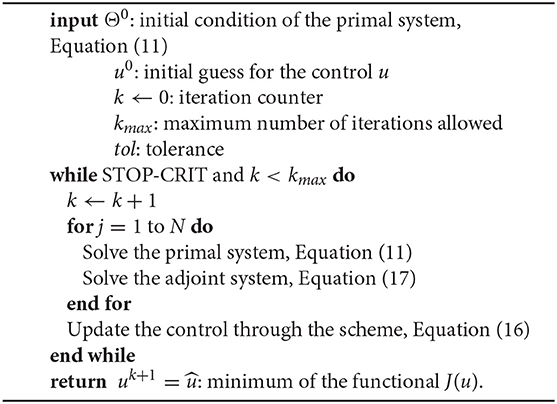
Algorithm 1. GD algorithm

In particular, we see that the control computation through the above algorithm requires, at each iteration k, to solve 2N non-linear differential equations (N for the variables θ_i and N for p_i). If we introduce the time-mesh of N_t points

$\begin{array}{l}0=t_0<t_1<\dots <t_{N_t}=T,t_m=t_0+m\frac{T}{N_t},m=1,\dots ,N_t,\end{array}$

at each time-step t_m this operation has a computational cost of ${O}(N^2)$ and the total computational complexity for the simulation of Equations (5) and (17) will then be ${O}(N_t{N}^2)$. If N is large, that is, if the number of oscillators in the network is considerable, this will rapidly become very expensive.

3.2. The Random Batch Method

In order to reduce the computational burden of GD for the optimization process (7), we propose a modification of this algorithm which includes the aforementioned RBM for the numerical simulation of the ODE systems Equations (5) and (17).

This technique, presented in Jin et al. (2020) for interacting particle systems, is based on the following simple idea: at each time step t_m = m·dt in the mesh we employ to solve the dynamics, we divide randomly the N particles into n small batches with size 2 ≤ P < N, denoted by C_q, q = 1, …, n, that is

$\begin{array}{ll}{C}_q=\{i_{q_1},\dots ,i_{q_P}\}\subset \left\{1,\dots ,N\right\},& \text{for all }q=1,\dots ,n\\ C_q\cap C_r=\varnothing ,& \text{for all }q,r=1,\dots ,n\\ {\displaystyle \bigcup _{q=1}^n}{C}_q=\left\{1,\dots ,N\right\}.\end{array}$

Notice that the last batch C_n may have size smaller than P if nP ≠ N.

Once this partition of {1, …, N} has been performed, we solve the dynamics by interacting only particles within the same batch. This gives the following algorithm for the numerical approximation of Equations (5) and (17):

ALGORITHM 2

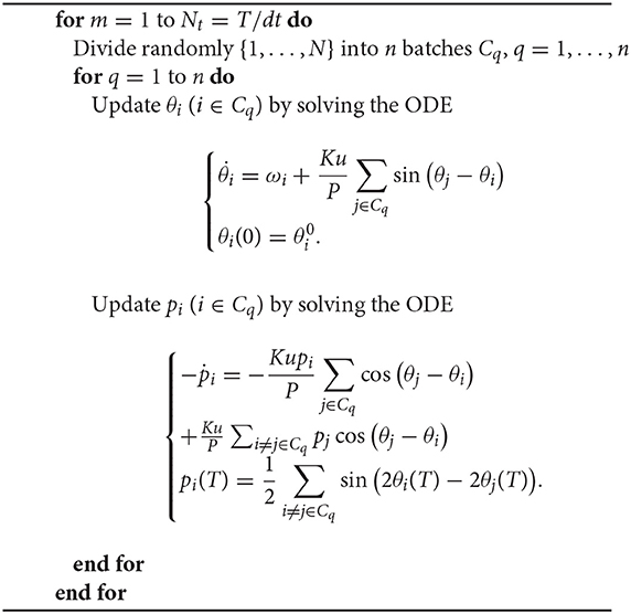
Algorithm 2. RBM algorithm

Regarding the complexity, note that random division into n batches can be implemented using random permutation. In Matlab, this can be done by using the function randperm(N). Then, the first P elements are considered to be in the first batch, the second P elements are in the second batch, and so on. According to the discussion presented in Jin et al. (2020), at each time step t_m this procedure yields to a cost of ${O}(PN)$ for approximating the dynamics with RBM.

If one is to simulate up to time T, the total number of time steps is N_t as in the algorithm above. Then, the total computational complexity for the simulation of Equations (5) and (17) is ${O}(P{N}_{t}N)$. Notice that, since P < N, this is always smaller than ${O}(N_t{N}^2)$.

Summarizing, with the GD and GD-RBM methodologies we obtain the following per-iteration costs:

• GD $\to {\mathrm{\text{cost}}}_{GD}={{C}}_{GD}{N}_t{N}^2$.

• GD-RBM $\to {\mathrm{\text{cost}}}_{GD-RBM}={{C}}_{GD-RBM}P{N}_{t}N$.

Therefore, independently of the value of N, employing RBM to simulate the dynamics in each iteration of GD yields improvements in terms of the computational cost.

For completeness, we shall mention that the above considerations are simply heuristic and would require a deeper analysis. As a matter of fact, to have a rigorous validation of the reduction in the computational complexity when using RBM one should have more precise information on the two constants ${{C}}_{GD}$ and ${{C}}_{GD-RBM}$, and be sure that the difference among them does not overwhelm the help that the batching procedure is providing.

At this regard, let us stress that the RBM method has been developed only recently in Jin et al. (2020) and, at present time, there is not a well-established qualitative analysis on its computational cost, going in more detail than what we mentioned above. The evidence that in our case of the Kuramoto model [Equation (5)] the GD-RBM method allows for a more efficient control computation, in particular for large oscillator networks, will then be given through the numerical simulations in section 4.

3.3. Convergence Analysis

To complete this section, let us briefly comment about the convergence properties of the GD methodology. It is nowadays classically known that the convergence rate of the GD algorithm is determined by the regularity of the objective function. In our case, since J(u) is L-smooth, that is

$\Vert \nabla J(u)-\nabla J(v){\Vert }_2\le L\Vert u-v{\Vert }_2,$

it can be proven that

$\begin{array}{ll}\Vert \nabla J(u^k){\Vert }_2\to 0\text{ as }k\to +\infty & (18)\end{array}$

and

$\begin{array}{ll}\Vert J(u^k)-J(\widehat{u}){\Vert }_2={O}\left(\frac{1}{k}\right),& (19)\end{array}$

where, we recall, $\hat{u}$ denotes the minimum of J(u) and the norm $\Vert ·{\Vert }_{L^2(0,T;ℝ)}$ has been defined in (8).

In particular, Equation (19) implies that for achieving ε-optimality, i.e., for obtaining $\Vert J(u^k)-J(\hat{u}){\Vert }_2<\epsilon$, the GD algorithm requires $k={O}({\epsilon }^{-1})$ iterations.

Combining this with the per-iteration costs we gave at the end of section 3.2, we can thus obtain the following total computational costs

• GD: ${O}\left(\frac{N_t{N}^2}{\epsilon }\right)$

• GD-RBM: ${O}\left(\frac{P{N}_{t}N}{\epsilon }\right)$,

and we can conclude that the GD-RBM approach will be more efficient than the standard GD one to solve our optimization problem. This is enhanced for large values of N and will be confirmed by our numerical simulations.

4. Numerical Simulations

We present here our numerical results for the control of N coupled oscillators described by the Kuramoto model (5), following the strategy previously described. This section is divided into two parts:

1. In a first moment, we will show that the optimization problem [Equation (7)] indeed allows to compute an effective control function which is capable to steer the Kuramoto model [Equation (5)] to a synchronized configuration. This will be done both for a strong coupling K > K^* [see Equation (4)] and for a weak coupling K < K^*. Besides, we will also briefly analyze the role of the parameter β in the optimization process. Finally, we will show the efficacy of our control strategy in the more realistic cases of a sparse interaction network and for a second-order Kuramoto model with damping.

2. Once the effectiveness of the control strategy we propose has been corroborated, we will compare the GD and GD-RBM algorithms for the minimization of J(u). In particular, we will show how the RBM approach allows to significantly reduce the computational complexity of the GD algorithm for the calculation of the control u, especially when considering oscillator networks of large dimension.

The oscillators are chosen such that their natural frequencies are given following the normal probability law

$\begin{array}{ll}f(\omega )=\frac{1}{5\sigma \sqrt{2\pi }}{e}^{-\frac{{\omega }^2}{2\sigma }},& (20)\end{array}$

with σ = 0.1. This means that the values of ω_min and ω_max are given respectively by

$\begin{array}{l}{\omega }_{\text{min}}={\displaystyle \underset{\omega \in ℝ}{\text{min}}}f(\omega )=0\\ {\omega }_{\text{max }}={\displaystyle \underset{\omega \in ℝ}{\text{max}}}f(\omega )=f(0)=\frac{2}{\sqrt{2\pi }}\end{array}$

and the coupling gain K which is necessary for synchronization in the absence of a control has to satisfy [see Equation (4)]

$\begin{array}{l}K>|{\omega }_{max}-{\omega }_{min}|=\frac{2}{\sqrt{2\pi }}.\end{array}$

The initial datum θ⁰ is chosen following a normal distribution as well, in such a way that $|{\theta }_i^0-{\theta }_j^0|<2\pi$ for all i, j = 1, …, N. Let us stress that this choice of θ⁰ allows the synchronization of the uncontrolled model, as it has been shown for instance in Dong and Xue (2013).

Without loss of generality, we considered the time horizon T = 3s for completing the synchronization. That is, we want all the oscillators in our model to reach the configuration [Equation (6)] in 3 s.

Finally, we used an explicit Euler scheme for solving the direct and adjoint dynamics (5) and (17) during the minimization of J(u), and we chose as a stopping criterion

$\begin{array}{ll}{e}_k:=\frac{\Vert \nabla J(u^k){\Vert }_2}{\Vert u^k{\Vert }_2}<\epsilon ,& (21)\end{array}$

with ε = 10⁻⁴, and where the notation ||·||₂ stands again for the L²(0, T ℝ)-norm defined in Equation (8). Let us stress that the stopping criterion [Equation (21)] is consistent with Equations (18) and (19).

4.1. Computation of the Optimal Control

In this section, we show that through the optimization problem [Equation (7)] we are able to compute an effective control function which is capable to steer the Kuramoto model [Equation (5)] to a synchronized configuration in a given time horizon T.

All the simulations have been performed in Matlab R2018a on a laptop with Intel Core i5−7200UCPU@2.50GHz × 4 processor and 7.7 GiB RAM.

We start by considering a simple scenario of N = 10 oscillators in an all-to-all coupled configuration and with a coupling gain K > K^*. Moreover, we set the penalization parameter β in Equation (7) to take the value β = 10⁻⁷.

When using the GD-RBM approach, the family of N = 10 oscillators has been separated into n = 5 batches of size P = 2.

In Figure 1-top, we show the evolution of the uncontrolled dynamics, which corresponds to taking u≡1 in Equation (5). As we can see, the oscillators are evolving toward a synchronized configuration, which is consistent with our choice of the coupling gain K. Nevertheless, synchronization is not reached in the short time horizon we are providing. At this regard, let us remark that, for the uncontrolled Kuramoto model with a sufficiently strong coupling gain, synchronization is expected to be reached only asymptotically, i.e., when t → +∞.

FIGURE 1

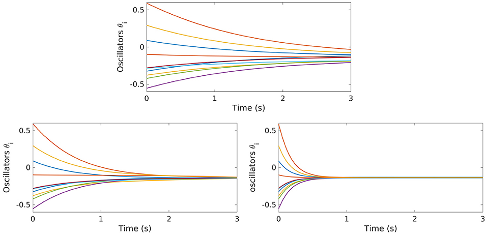
Figure 1. Top: Evolution of the free dynamics of the Kuramoto model [Equation (5)] with N = 10 oscillators. Bottom: Evolution of the controlled dynamics of the Kuramoto model [Equation (5)] with N = 10 oscillators. The control function $\hat{u}$ is obtained with the GD (left) and the GD-RBM (right) approach.

In Figure 1-bottom, we show the evolution of the same dynamics, this time under the action of the control function u computed through the minimization of J(u). The subplot on the left corresponds to the simulations done with the GD approach, while the one on the right is done employing GD-RBM. We can clearly see how, in both cases, the oscillators are all synchronized at the final time T = 3s. This means that both algorithms managed to compute an effective control.

In Figure 2, we show the convergence of the error in logarithmic scale when applying both the GD and GD-RBM approach. We can appreciate how, in the case of GD-RBM, this convergence is not monotonic as it is for the GD algorithm. This, however, is not surprising due to the stochastic nature of the RBM methodology.

FIGURE 2

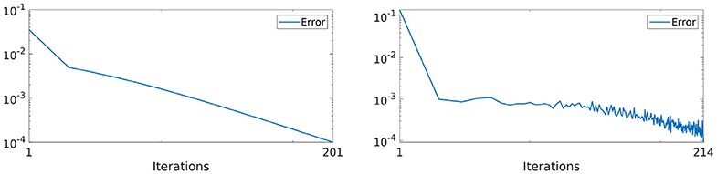
Figure 2. Convergence of the error e_k [see Equation (21)] in logarithmic scale with the GD (left) and GD-RBM (right) algorithm.

In Figure 3, we display the behavior of the control function $\hat{u}$ computed via the GD-RBM algorithm. We can see how, at the beginning of the time interval we are considering, this control is close to one and it is increasing with a small slope. On the other hand, this growth becomes more pronounced as we get closer to the final time T = 3s.

FIGURE 3

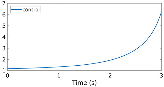
Figure 3. Control function $\hat{u}$ obtained through the GD-RBM algorithm applied to the Kuramoto model [Equation (5)] with N = 10 oscillators.

Notice that, in Equation (5), $\hat{u}$ enters as a multiplicative control which modifies the strength of the coupling K. Hence, according to the profile displayed in Figure 2, the control function $\hat{u}$ we computed is initially letting the system evolving following its natural dynamics. Then, as the time evolves toward the horizon T = 3s, $\hat{u}$ enhances the coupling strength K in order to reach the desired synchronized configuration [Equation (6)].

Finally, notice also that the control $\hat{u}$ is always positive. This is actually not surprising, if one takes into account the following observation.

In the Kuramoto model, in order to reach synchronization the coupling strength K needs to be positive. Otherwise, the system would converge to a desynchronized configuration (see Hong and Strogatz, 2011). Moreover, according to the model [Equation (5)], if we start from K > 0, in order to maintain this coupling positive $\hat{u}$ has to remain positive as well.

Recall that $\hat{u}$ is computed minimizing the functional [Equation (7)], in which the second term is a measurement of the level of synchronization in the model. Hence, since negative values of $\hat{u}$ would lead to desynchronization and to the corresponding increasing of the functional, these values remain automatically excluded during the minimization process.

Let us now discuss briefly the role of the penalization parameter β in the computation of the optimal control. To this end, we have run simulations with different values of β = 10⁻², 10⁻³, 10⁻⁴ and 10⁻⁷.

As we already mentioned in section 3, in the cost functional [Equation (7)] β is a (usually small) penalization parameter which allows to tune the norm of the optimal control $\hat{u}$, that is, the amount of energy that the control introduces into the system. Roughly speaking, the smaller is β the larger will be $\hat{u}$.

This is clearly seen in Figure 4. In particular, we can appreciate how, for β = 10⁻², the computed control remains smaller than in the other cases.

FIGURE 4

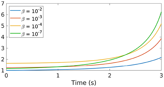
Figure 4. Control function $\hat{u}$ obtained through the GD-RBM algorithm applied to the Kuramoto model [Equation (5)] with N = 10 oscillators and different values of β.

We already mentioned above that the effect of the control in Equation (5) is to enhance synchronization by modifying the strength of the coupling K. Hence, we can expect that, if $\hat{u}$ is small (in particular, if it remains close to one), the synchronization properties of the Kuramoto model [Equation (5)] will be worst than when applying a larger control. At this regard, let us recall that the level of synchronization in Equation (5) can be analyzed in terms of the quantity

$r(t):=\left|\frac{1}{N}{\displaystyle \sum _{j=1}^N{e}^{i{\theta }_j(t)}}\right|,$

measuring the coherence of the oscillator population (see Acebrón et al., 2005). In particular we always have 0 ≤ r(t) ≤ 1 and synchronization arises when r reaches the value one.

In Figure 5, we show the behavior of r(t) with respect to the parameter β. On the one hand, in all the cases displayed we can clearly see that r(T) = 1. This means that all the computed controls will be effective to steer the system [Equation (5)] to its synchronized configuration at time T. On the other hand, we can also notice how, when decreasing β, the function r(t) reaches the value one faster, meaning that the corresponding control is expected to yield to better synchronization properties.

FIGURE 5

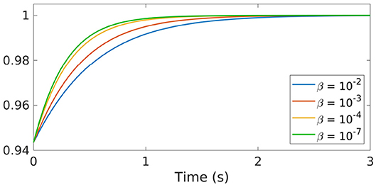
Figure 5. Behavior of the synchronization function r(t) corresponding to the controlled dynamics [Equation (5)] for different values of the parameter β.

Let us now conclude this section by showing that the control strategy that we propose in this paper is effective also in situations in which the coupling gain among the oscillators is too weak to ensure synchronization for the uncontrolled dynamics of the Kuramoto model. This corresponds to taking K < K^* [see Equation (4)]. In particular, we will consider the case K < 0 in which the system is known to converge to a desynchronized configuration (see Hong and Strogatz, 2011).

For simplicity, in these simulations we only employed the GD-RBM algorithm, since using the GD approach we would obtain analogous results.

We can see in Figure 6 how, in this case of a negative coupling gain, the uncontrolled dynamics is diverging as t increases. On the other hand, when applying the control $\hat{u}$, the system is once again steered to a synchronized configuration.

FIGURE 6

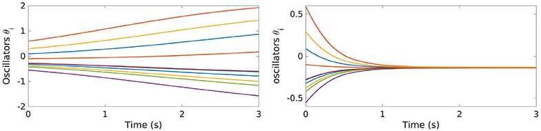
Figure 6. Evolution of the uncontrolled (left) and controlled (right) dynamics of the Kuramoto model [Equation (5)] with N = 10 oscillators and K < 0.

At this regard, it is also interesting to observe that, this time, the control function we obtained is always negative (see Figure 7). This fact is not surprising, if we recall that in Equation (5) the control acts by modifying the coupling gain K so that the oscillators are all synchronized at time T and that, for the uncontrolled dynamics, synchronization requires K > 0.

FIGURE 7

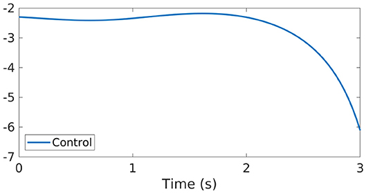
Figure 7. Control function $\hat{u}$ obtained through the GD-RBM algorithm applied to the Kuramoto model [Equation (5)] with N = 10 oscillators and K < 0.

Let us now complement our analysis by briefly showing the efficacy of our control strategy in a couple of more complex and realistic situations.

4.1.1. The Case of a Sparse Interaction Network

We start by considering the case of a sparse interaction network in our Kuramoto model [Equation (5)]. In other words, we are considering here the following system

$\begin{array}{ll}\begin{array}{l}\{\begin{array}{l}{\dot{\theta }}_i(t)={\omega }_i+\frac{Ku(t)}{N}{\displaystyle \sum _{j=1}^N{a}_{i,j}}\text{ sin }({\theta }_j(t)-{\theta }_i(t)),\hfill \\ i=1,\dots ,N,t>0\hfill \\ {\theta }_i(0)={\theta }_i^0,\hfill \end{array}\hfill \end{array}& (22)\end{array}$

with

$a_{i,j}=\{\begin{array}{ll}1,\hfill & \text{ if }{\theta }_i\text{ is connected with }{\theta }_j\hfill \\ 0,\hfill & \text{ if }{\theta }_i\text{ is not connected with }{\theta }_j\hfill \end{array}$

A schematic representation of the network considered in our simulations is given in Figure 8, in which the blue dots correspond to a_{i, j} = 1.

FIGURE 8

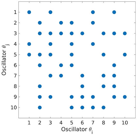
Figure 8. Sparse interaction scheme for the Kuramoto model [Equation (22)].

The simulations have been performed with the same initial datum and time horizon we considered in our previous experiments. Moreover, we addressed here only the case of a strong coupling gain K > K^*. The minimization of the functional J(u) has been performed with the GD algorithm.

In Figure 9, we show the evolution of the uncontrolled and controlled dynamics. As we can see, while in the absence of a control the oscillators are evolving toward a desynchronized configuration, when applying the control function we computed the system still reaches synchronization at time T.

FIGURE 9

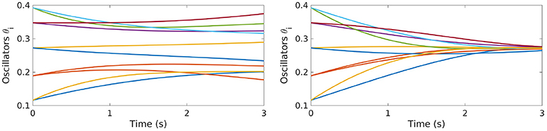
Figure 9. Evolution of the uncontrolled (left) and controlled (right) dynamics of the Kuramoto model [Equation (22)] with N = 10 oscillators, K > K^* and interactions as in Figure 8.

The control function obtained for these numerical experiments is plotted in Figure 10. We can observe how, differently from what is shown in Figures 3, 4, this time $\hat{u}$ reaches larger values. This is not surprising, if we consider that now our model has a lower level of interactions and if we recall our previous discussion on how our control affects the Kuramoto dynamics.

FIGURE 10

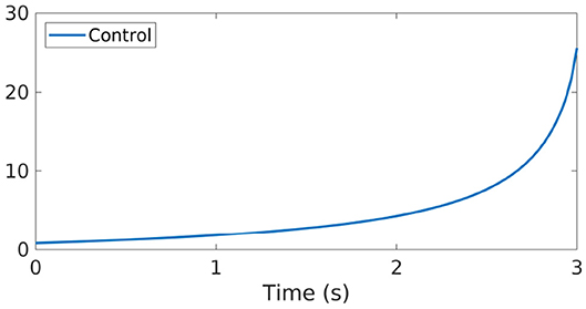
Figure 10. Control function $\hat{u}$ for the Kuramoto model (22) with N = 10 oscillators, K > K^* and interactions as in Figure 8.

4.1.2. A Second-Order Model With Damping

We consider here the second-order Kuramoto model with damping

$\{\begin{array}{l}{\ddot{\theta }}_i(t)+{\dot{\theta }}_i(t)={\omega }_i+\frac{Ku(t)}{N}{\displaystyle \sum _{j=1}^N\text{sin}}({\theta }_j(t)-{\theta }_i(t)),\hfill \\ i=1,\dots ,N,t>0\hfill \\ {\theta }_i(0)={\theta }_i^0,{\dot{\theta }}_i(0)={\theta }_i^1,\hfill \end{array}$

which can be rewritten as the following first-order system

$\begin{array}{ll}\{\begin{array}{l}{\dot{\theta }}_i(t)={\xi }_i(t),\hfill \\ i=1,\dots ,N,t>0\hfill \\ {\dot{\xi }}_i(t)=-{\xi }_i(t)+{\omega }_i+\frac{Ku(t)}{N}{\displaystyle \sum _{j=1}^N\text{sin}}({\theta }_j(t)-{\theta }_i(t)),\hfill \\ i=1,\dots ,N,t>0\hfill \\ {\theta }_i(0)={\theta }_i^0,{\xi }_i(0)={\theta }_i^1.\hfill \end{array}& (23)\end{array}$

In the context of power grids, this model has been firstly introduced in the work (Filatrella et al., 2008). Later on, in Schmietendorf et al. (2014), it has been extended to consider more complex scenarios in which the dynamics of the voltage amplitude is taken into account.

Also in this case, we are interested in computing a control capable to steer the system to the synchronized configuration [Equation (6)]. This can be done once again by solving the optimal control problem [Equation (7)], this time under the dynamics [Equation (23)].

The simulations have been performed with the same initial datum ${\Theta }^0={({\theta }_i^0)}_{i=1}^N$ we considered in our previous experiments and with ${\Theta }^1={({\theta }_i^1)}_{i=1}^N={(0,0,\dots ,0)}^{\top }$. The time horizon is once again T = 3s. Moreover, we addressed here both the cases of a strong coupling gain K > K^* and of a negative one K < 0. The minimization of the functional J(u) has been performed with the GD algorithm.

At this regard, we shall mention that, in Tumash et al. (2019), the GD methodology has been applied to obtain synchronization in a sparse network of Kuramoto oscillators with damping under the action of an additive control, i.e., the following model

$\{\begin{array}{l}{\dot{\theta }}_i(t)={\xi }_i(t),\hfill \\ i=1,\dots ,N,t>0\hfill \\ {\dot{\xi }}_i(t)=-{\xi }_i(t)+{\omega }_i+\frac{K}{N}{\displaystyle \sum _{j=1}^N{a}_{i,j}}\text{sin}({\theta }_j(t)-{\theta }_i(t))+u_i(t),\hfill \\ i=1,\dots ,N,t>0\hfill \\ {\theta }_i(0)={\theta }_i^0,{\xi }_i(0)={\theta }_i^1.\hfill \end{array}$

The advantages and disadvantages of this additive control action with respect to the multiplicative one we propose have been discussed in section 3. In particular, our control strategy allows us to deal also with negative coupling gain K < 0, while in Tumash et al. (2019) only K > 0 has been considered.

As a matter of fact, in Figure 11, we show the evolution of the uncontrolled and controlled dynamics, for K > K^* and K < 0, respectively. Also in this case, the proposed control strategy allows us to compute an effective control function $\hat{u}$ which steers the system to a synchronized configuration in time T.

FIGURE 11

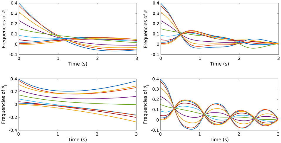
Figure 11. Evolution of the uncontrolled (left) and controlled (right) dynamics of the Kuramoto model [Equation (23)] with N = 10 oscillators and K > K^* (top) and K < 0 (bottom).

Finally, the control functions obtained for these numerical experiments are plotted in Figure 12. Also in these cases we can observe different behaviors than what is shown in Figures 3, 4. In particular, this time $\hat{u}$ changes sign in the time horizon (0, T). At this regard, let us mention that for the second-order Kuramoto model [Equation (23)], due to the presence of the damping term, our previous considerations on the sign of the control do not apply anymore. Hence, it is not surprising to obtain a behavior as the one displayed.

FIGURE 12

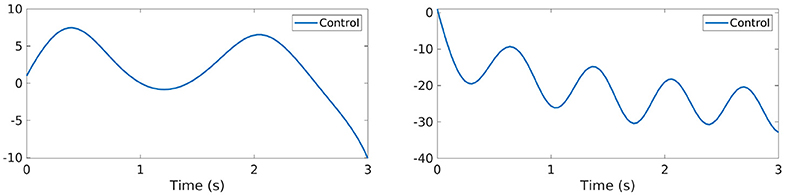
Figure 12. Control function $\hat{u}$ for the Kuramoto model [Equation (23)] with N = 10 oscillators and K > K^* (left) and K < 0 (right).

4.2. Comparison of GD and GD-RBM

We conclude this section on the numerical experiments by comparing the performances of the GD and GD-RBM algorithms for the computation of the optimal control $\hat{u}$.

To this end, we run simulations for increasing values of N, namely N = 10, 50, 100, 250, 1, 000. As before, we chose a time horizon T = 3s and a penalization parameter β = 10⁻⁷. Moreover, we considered the case of a large coupling gain K > K^*.

In what follows, we focus only on the simple case of the first-order Kuramoto model [Equation (5)] with an all-to-all interaction network. We will briefly comment about possible extensions to the more realistic scenarios described in sections 4.1.1 and 4.1.2 in the last part of this paper, devoted to conclusions and open problems.

In Table 1 (see also Figure 13), we collected the computational times required by the two methodologies to solve the optimization problem [Equation (7)]. At this regard, let us stress that the values contained in the table do not represent the time required by the control to synchronize the network which, we recall, is a fixed external input in our algorithms.

TABLE 1

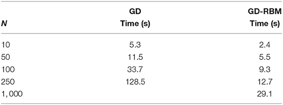
Table 1. Computational times required by the GD and GD-RBM algorithm to compute the optimal control $\hat{u}$ with increasing values of N.

FIGURE 13

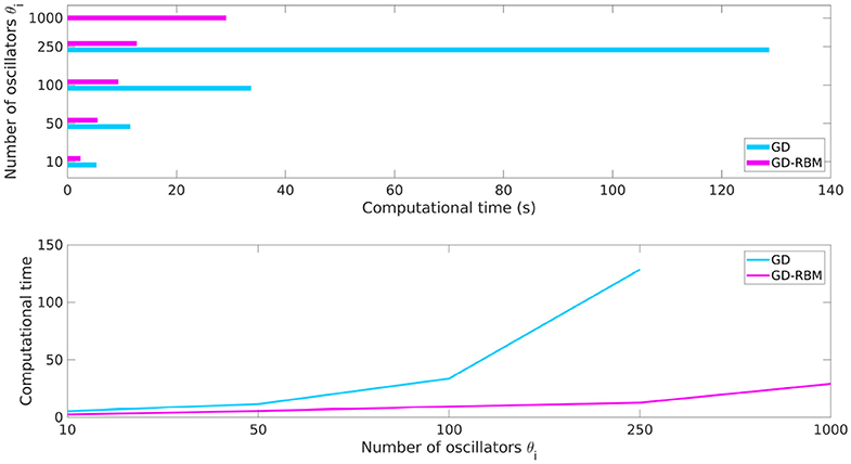
Figure 13. Computational times required by the GD and GD-RBM algorithm to compute the optimal control $\hat{u}$ with increasing values of N.

Our simulations show how, for low values of N, the two approaches have similar behaviors. Nevertheless, when increasing the number of oscillators in our system, the advantages of the GD-RBM methodology with respect to GD become evident. In particular, the growth of the computational time for GD-RBM is significantly less pronounced than for GD. As a matter of fact, in the case of N = 1, 000 oscillators, we decided not to perform the simulations with the GD algorithm since its behavior with smaller values of N already suggested that this experiment would be computationally too expensive.

On the other hand, even with N = 1, 000 oscillators in the system, the GD-RBM approach turns out to be able to compute an effective control for the Kuramoto model [Equation (5)] (see Figure 14) in about 29 s.

FIGURE 14

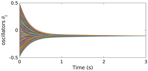
Figure 14. Evolution of the controlled dynamics of the Kuramoto model (5) with N = 1, 000 oscillators. The control has been computed with the GD-RBM algorithm.

5. Conclusions

This paper deals with the synchronization of coupled oscillators described by the Kuramoto model. In particular, we design a unique scalar control function u(t) capable of steering a N-dimensional network of oscillators to a synchronized configuration in a finite time horizon. This is done following a standard optimal control approach and obtaining the function u(t) via the minimization of a suitable cost functional.

With this approach, we computed a control which acts as a multiplicative force enhancing the coupling between the oscillators in the network, thus favoring the synchronization in the time horizon provided.

To carry out this minimization process, we used a Gradient Descent (GD) methodology, commonly employed in the optimal control community, which we have coupled with the novel RBM for a more efficient numerical resolution of the Kuramoto dynamics. The main purpose of this work has been to show how the introduction of RBM into GD may yield considerable improvement in term of the computational complexity, in particular for large oscillator networks.

Our simulations results have shown the following main facts:

• The proposed control strategy is indeed effective to reach a synchronized configuration in a finite time horizon. Moreover, it allows to deal efficiently with large networks of oscillators (namely, N = 1, 000) and with the case of a low coupling gain in the network, when the uncontrolled dynamics is not expected to reach a synchronized configuration.

• For large values of N, the inclusion of RBM into the GD algorithm significantly reduces the computational burden for the control computation, thus allowing to deal with high-dimensional oscillators networks in a more efficient way.

In conclusion, the study conducted in this paper suggests that the proposed methodology, based on the combination of the standard GD optimization algorithm with the novel RBM method for the numerical resolution of multi-agent dynamics, may help in significantly reduce the computational complexity for the control computation of the Kuramoto model, in particular in the case of a high-dimensional system.

At this regard, we shall stress that the analysis in this paper has been developed mostly in a simplified framework of a network with all-to-all coupling, in which the oscillators are all interacting among themselves. The following interesting questions remain unaddressed:

• To study whether our methodology remains valid in more complex scenarios of networks with sparse interaction topologies, perturbations due to disconnections, or rewiring. In particular, it would be relevant to determine if the reduction in computational complexity that we obtained through the GD-RBM algorithm is related with the density of the network or, instead, this approach allows to deal efficiently also with the case of a low number of interactions. A starting point for this analysis would be to determine whether the GD-RBM methodology can be successfully applied in the scenarios we addressed in sections 4.1.1 and 4.1.2.

• To analyze what happens if, instead of selecting the oscillators uniformly at random during the batching process in RBM, we organize them in groups with similar frequencies. At this regard, it would be important to understand if the methodology we propose is still effective or, instead, some modifications need to be introduced.

• To analyze if our methodology may be applied also in different framework than the ones considered in this paper. For instance, a similar formalism than the one we have proposed has been developed for computing rare-events in oscillator networks due to noise. See for instance Hindes and Schwartz, 2018; Hindes et al., 2019. In these mentioned contributions, the objective functional is the probability for a rare event to happen. The actions are more complicated than the simple L²-norm, but the batch techniques we employed may be useful in this context as well.

All these are key open problem which will be considered in future works.

Data Availability Statement

The raw data supporting the conclusions of this article will be made available by the authors, without undue reservation, to any qualified researcher.

Author Contributions

UB carried out the calculations and simulation work and drafted the manuscript. EZ suggested the methodology, reviewed the manuscript, and supervised the overall work.

Funding

This project has received funding from the European Research Council (ERC) under the European Union's Horizon 2020 research and innovation programme (grant agreement NO. 694126-DyCon). The work of both authors was partially supported by the Grant MTM2017-92996-C2-1-R COSNET of MINECO (Spain) and by the Air Force Office of Scientific Research (AFOSR) under Award NO. FA9550-18-1-0242. The work of EZ was partially funded by the Alexander von Humboldt-Professorship program, the European Unions Horizon 2020 research and innovation programme under the Marie Sklodowska-Curie grant agreement No.765579-ConFlex, the Grant ICON-ANR-16-ACHN-0014 of the French ANR and the Transregio 154 Project Mathematical Modelling, Simulation and Optimization Using the Example of Gas Networks of the German DFG.

Conflict of Interest

The authors declare that the research was conducted in the absence of any commercial or financial relationships that could be construed as a potential conflict of interest.

Acknowledgments

The authors wish to acknowledge Jesús Oroya and Dongnam Ko (Chair of Computational Mathematics, Fundación Deusto, Bilbao, Spain) and Eneko Unamuno (Mondragón University, Spain) for interesting discussion on the topics of the present paper.

References

Acebrón, J. A., Bonilla, L. L., Vicente, C. J. P., Ritort, F., and Spigler, R. (2005). The Kuramoto model: a simple paradigm for synchronization phenomena. Rev. Modern Phys. 77:137. doi: 10.1103/RevModPhys.77.137

CrossRef Full Text | Google Scholar

Ben-Naim, E. (2005). Opinion dynamics: rise and fall of political parties. Europhys. Lett. 69:671. doi: 10.1209/epl/i2004-10421-1

CrossRef Full Text | Google Scholar

Biccari, U., Ko, D., and Zuazua, E. (2019). Dynamics and control for multi-agent networked systems: a finite-difference approach. Math. Models Methods Appl. Sci. 29, 755–790. doi: 10.1142/S0218202519400050

CrossRef Full Text | Google Scholar

Bottou, L., Curtis, F., and Nocedal, J. (2018). Optimization methods for large-scale machine learning. SIAM Rev. 60, 223–311. doi: 10.1137/16M1080173

CrossRef Full Text | Google Scholar

Buck, J. (1988). Synchronous rhythmic flashing of fireflies II. Quart. Rev. Bio. 63, 265–289. doi: 10.1086/415929

PubMed Abstract | CrossRef Full Text | Google Scholar

Chassin, D. P., and Posse, C. (2005). Evaluating north American electric grid reliability using the Barabási-Albert network model. Phys. A 355, 667–677. doi: 10.1016/j.physa.2005.02.051

CrossRef Full Text | Google Scholar

Chopra, N., and Spong, M. W. (2005). “On synchronization of Kuramoto oscillators,” in Proceedings of the 44th IEEE Conference on Decision and Control (Seville: IEEE), 3916–3922. doi: 10.1109/CDC.2005.1582773

CrossRef Full Text | Google Scholar

Chopra, N., and Spong, M. W. (2006). “Passivity-based control of multi-agent systems,” in Advances in Robot Control, eds S. Kawamura and M. Svinin (Berlin, Heidelberg: Springer), 107–134. doi: 10.1007/978-3-540-37347-6_6

CrossRef Full Text | Google Scholar

Chopra, N., and Spong, M. W. (2009). On exponential synchronization of Kuramoto oscillators. IEEE Trans. Autom. Control 54, 353–357. doi: 10.1109/TAC.2008.2007884

CrossRef Full Text | Google Scholar

Dong, J.-G., and Xue, X. (2013). Synchronization analysis of Kuramoto oscillators. Commun. Math. Sci. 11, 465–480. doi: 10.4310/CMS.2013.v11.n2.a7

CrossRef Full Text | Google Scholar

Dörfler, F., and Bullo, F. (2010). Synchronization of power networks: Network reduction and effective resistance. IFAC Proc. Vol. 43, 197–202. doi: 10.3182/20100913-2-FR-4014.00048

CrossRef Full Text | Google Scholar

Dörfler, F., Chertkov, M., and Bullo, F. (2013). Synchronization in complex oscillator networks and smart grids. Proc. Nat. Acad. Sci. U.S.A. 110, 2005–2010. doi: 10.1073/pnas.1212134110

PubMed Abstract | CrossRef Full Text | Google Scholar

Filatrella, G., Nielsen, A. H., and Pedersen, N. F. (2008). Analysis of a power grid using a Kuramoto-like model. Europe. Phys. J. B 61, 485–491. doi: 10.1140/epjb/e2008-00098-8

CrossRef Full Text | Google Scholar

Ha, S.-Y., Kim, H. K., and Park, J. (2015). Remarks on the complete synchronization of Kuramoto oscillators. Nonlinearity 28:1441. doi: 10.1088/0951-7715/28/5/1441

CrossRef Full Text | Google Scholar

Ha, S.-Y., Kim, H. K., and Ryoo, S. W. (2016). Emergence of phase-locked states for the Kuramoto model in a large coupling regime. Commun. Math. Sci. 14, 1073–1091. doi: 10.4310/CMS.2016.v14.n4.a10

CrossRef Full Text | Google Scholar

Hindes, J., Jacquod, P., and Schwartz, I. B. (2019). Network desynchronization by non-Gaussian fluctuations. Phys. Rev. E 100:052314. doi: 10.1103/PhysRevE.100.052314

PubMed Abstract | CrossRef Full Text | Google Scholar

Hindes, J., and Schwartz, I. B. (2018). Rare slips in fluctuating synchronized oscillator networks. Chaos 28:071106. doi: 10.1063/1.5041377

PubMed Abstract | CrossRef Full Text | Google Scholar

Hong, H., and Strogatz, S. H. (2011). Kuramoto model of coupled oscillators with positive and negative coupling parameters: an example of conformist and contrarian oscillators. Phys. Rev. Lett. 106:054102. doi: 10.1103/PhysRevLett.106.054102

PubMed Abstract | CrossRef Full Text | Google Scholar

Jadbabaie, A., Motee, N., and Barahona, M. (2004). “On the stability of the Kuramoto model of coupled nonlinear oscillators,” in Proc. 2004 American Control Conference (Boston, MA: IEEE), 4296–4301. doi: 10.23919/ACC.2004.1383983

CrossRef Full Text | Google Scholar

Jin, S., Li, L., and Liu, J.-G. (2020). Random Batch Methods (RBM) for interacting particle systems. J. Comput. Phys. 400:108877. doi: 10.1016/j.jcp.2019.108877

CrossRef Full Text | Google Scholar

Kuramoto, Y. (1975). “Self-entrainment of a population of coupled non-linear oscillators,” in International symposium on Mathematical Problems in Theoretical Physics (Kyoto: Springer), 420–422. doi: 10.1007/BFb0013365

CrossRef Full Text | Google Scholar

Markdahl, J., Thunberg, J., and Goncalves, J. (2020). High-dimensional Kuramoto models on Stiefel manifolds synchronize complex networks almost globally. Automatica 113:108736. doi: 10.1016/j.automatica.2019.108736

CrossRef Full Text | Google Scholar

Mehyar, M., Spanos, D., Pongsajapan, J., Low, S. H., and Murray, R. M. (2005). “Distributed averaging on asynchronous communication networks,” in Proceedings of the 44th IEEE Conference on Decision and Control (Seville: IEEE), 7446–7451. doi: 10.1109/CDC.2005.1583363

CrossRef Full Text | Google Scholar

Nabi, A., and Moehlis, J. (2011). Single input optimal control for globally coupled neuron networks. J. Neural Eng. 8:065008. doi: 10.1088/1741-2560/8/6/065008

PubMed Abstract | CrossRef Full Text | Google Scholar

Nesterov, Y. (2004). Applied Optimization. Introductory Lectures on Convex Optimization: A Basic Course. Boston, MA; Dordrecht; London: Kluwer Academic Publishers. doi: 10.1007/978-1-4419-8853-9

CrossRef Full Text | Google Scholar

Nocedal, J., and Wright, S. (2006). Numerical optimization. Springer Series in Operations Research and Financial Engineering. Springer Science & Business Media.

Google Scholar

Olfati-Saber, R. (2006). Flocking for multi-agent dynamic systems: algorithms and theory. IEEE Trans. Autom. Control 51, 401–420. doi: 10.1109/TAC.2005.864190

CrossRef Full Text | Google Scholar

Olfati-Saber, R., Fax, J. A., and Murray, R. M. (2007). Consensus and cooperation in networked multi-agent systems. Proc. IEEE 95, 215–233. doi: 10.1109/JPROC.2006.887293

CrossRef Full Text | Google Scholar

Rosenblum, M., and Pikovsky, A. (2004). Delayed feedback control of collective synchrony: an approach to suppression of pathological brain rhythms. Phys. Rev. E 70:041904. doi: 10.1103/PhysRevE.70.041904

PubMed Abstract | CrossRef Full Text | Google Scholar

Sachtjen, M., Carreras, B., and Lynch, V. (2000). Disturbances in a power transmission system. Phys. Rev. E 61:4877. doi: 10.1103/PhysRevE.61.4877

PubMed Abstract | CrossRef Full Text | Google Scholar

Schmidhuber, J. (2015). Deep learning in neural networks: an overview. Neural Netw. 61, 85–117. doi: 10.1016/j.neunet.2014.09.003

PubMed Abstract | CrossRef Full Text | Google Scholar

Schmietendorf, K., Peinke, J., Friedrich, R., and Kamps, O. (2014). Self-organized synchronization and voltage stability in networks of synchronous machines. Eur. Phys. J. Spec. Top. 223, 2577–2592. doi: 10.1140/epjst/e2014-02209-8

CrossRef Full Text | Google Scholar

Sepulchre, R., Paley, D., and Leonard, N. (2005). “Collective motion and oscillator synchronization,” in Cooperative Control (Berlin: Springer), 189–205. doi: 10.1007/978-3-540-31595-7_11

CrossRef Full Text | Google Scholar

Shalev-Shwartz, S., and Zhang, T. (2014). “Accelerated proximal stochastic dual coordinate ascent for regularized loss minimization,” in International Conference on Machine Learning (Beijing), 64–72.

Google Scholar

Strogatz, S. H. (2001). Exploring complex networks. Nature 410, 268–276. doi: 10.1038/35065725

PubMed Abstract | CrossRef Full Text | Google Scholar

Strogatz, S. H., Abrams, D. M., McRobie, A., Eckhardt, B., and Ott, E. (2005). Crowd synchrony on the millennium bridge. Nature 438, 43–44. doi: 10.1038/438043a

PubMed Abstract | CrossRef Full Text | Google Scholar

Sun, J., Bollt, E. M., and Nishikawa, T. (2009). Master stability functions for coupled nearly identical dynamical systems. Europhys. Lett. 85:60011. doi: 10.1209/0295-5075/85/60011

PubMed Abstract | CrossRef Full Text | Google Scholar

Taylor, D., Skardal, P. S., and Sun, J. (2016). Synchronization of heterogeneous oscillators under network modifications: perturbation and optimization of the synchrony alignment function. SIAM J. Appl. Math. 76, 1984–2008. doi: 10.1137/16M1075181

PubMed Abstract | CrossRef Full Text | Google Scholar

Toscher, A., and Jahrer, M. (2010). Collaborative filtering applied to educational data mining. In: Proceedings of the KDD 2010 Cup 2010 Workshop: Knowledge Discovery in Educational Data, 13–23.

Google Scholar

Trélat, E. (2005). Contrôle Optimal: Théorie & Applications. Vuibert, Collection Mathématiques Concrétes.

Google Scholar

Tröltzsch, F. (2010). Optimal control of partial differential equations: theory, methods, and applications. Am. Math. Soc. 112.

Google Scholar

Tukhlina, N., Rosenblum, M., Pikovsky, A., and Kurths, J. (2007). Feedback suppression of neural synchrony by vanishing stimulation. Phys. Rev. E 75:011918. doi: 10.1103/PhysRevE.75.011918

PubMed Abstract | CrossRef Full Text | Google Scholar

Tumash, L., Olmi, S., and Schöll, E. (2019). Stability and control of power grids with diluted network topology. Chaos 29:123105. doi: 10.1063/1.5111686

PubMed Abstract | CrossRef Full Text | Google Scholar

Walker, T. J. (1969). Acoustic synchrony: two mechanisms in the snowy tree cricket. Science 166, 891–894. doi: 10.1126/science.166.3907.891

PubMed Abstract | CrossRef Full Text | Google Scholar

Wiesenfeld, K., Colet, P., and Strogatz, S. H. (1998). Frequency locking in Josephson arrays: connection with the Kuramoto model. Phys. Rev. E 57:1563. doi: 10.1103/PhysRevE.57.1563

CrossRef Full Text | Google Scholar

Winfree, A. T. (1967). Biological rhythms and the behavior of populations of coupled oscillators. J. Theor. Biol. 16, 15–42. doi: 10.1016/0022-5193(67)90051-3

PubMed Abstract | CrossRef Full Text | Google Scholar