Steam Turbine—Quo Vadis?

Introduction

It would be presumptuous of the author to claim that this research contains never-before-seen, utterly innovative, and unique material on the subject matter, i.e., steam turbines. There has been not much in terms of truly original contribution to steam turbine thermodynamics since Stodola’s century-old masterpiece on steam and gas turbines (Stodola, 1927). Huge strides made since then depended to a large extent on development of alloy steels, mechanical designs, and manufacturing techniques to push steam conditions higher (and back pressures lower). For more in-depth information, refer to the recent monographs by the author and references cited therein (Gülen, 2019a; Gülen, 2019b). While in this day and age most information is available online and only “one click” away, the author strongly recommends resisting the urge to “google” unfamiliar concepts and terminology and instead turn to true and tested references. His recommendations are the introductory thermodynamics book by Moran and Shapiro (1998)1988 and the proverbial industry “bible” Steam by The Babcock & Wilcox Company (Steam, 2015). Especially for boiler thermodynamics, design and hardware, Chapters 4, 19, and 22 of Steam (2015) constitute possibly the best resource for laypersons as well as practitioners. A crash course on conventional steam cycle thermodynamics and heat and mass balance analysis can be found in Chapter 2 of the same source. For the practical aspects of steam turbine design and operability itself, Leyzerovich’s book is a good source¹ (Leyzerovich, 2008).

The intent of the present article is to provide the reader with a first principles-based look at the state-of-the-art in steam turbine design from two perspectives, i.e., performance and operability. This will enable the reader to assess many claims made in trade publications and even in archival journals about the capabilities of steam turbines and competing technologies (e.g., most prominently these days, supercritical CO₂ cycles), which are frequently colored by marketing hyperbole and hidden behind impenetrable technical jargon.

Steam turbines for electric power generation are available in three major configurations:

1 ‐as the sole prime mover in a fossil fuel (in most cases coal) fired boiler-turbine power plant;

2 ‐as the sole prime mover in a nuclear power plant;

3 ‐as one of the prime movers in a gas turbine “combined cycle” power plant with a (steam) bottoming cycle.

The first two can be grouped under the heading of “conventional steam” power plant. The difference between the two lies in the nature of the steam boiler, which in the case of a nuclear power plant is the nuclear reactor. One can even add the concentrated solar power (CSP) plant into this group. After all, a CSP power plant is a boiler-turbine power plant as well. In this case, the steam boiler’s heat source is solar radiation (i.e., it is unfired, just like the nuclear reactor).

By the same token, gas turbine combined cycle (GTCC) “bottoming” cycle² can be considered as a special case of waste heat recovery. In this case, the “waste heat” in question is the thermal energy of gas turbine exhaust gas, which otherwise would be dumped into the atmosphere (i.e., “wasted”). Industrial facilities in general and chemical process plants in particular (e.g., refineries) have various sources of waste heat of different quality (i.e., temperature) and quantity (i.e., kWth). In many instances, use is already made of that waste heat via small industrial turbines (e.g., backpressure units rated at a few megawatts) to meet power demand of users inside the industrial facility. Nonetheless, when it comes to utility scale electric power generation (i.e., 100 MWe or higher), GTCC bottoming cycle is the only viable waste heat recovery technology.

While the thermodynamic cycle governing the steam turbine operation is the Rankine cycle in either case, there are some important differences in steam turbine design as follows.

1 In a boiler-turbine (fired or unfired, i.e., nuclear or CSP) power plant, steam is generated at a single pressure level and feed water heating is used to enhance thermal efficiency.

2 In modern GTCC power plants, steam is generated at three pressure levels (in the heat recovery steam generator, HRSG) and feed water heating is avoided for maximum combined cycle efficiency.

Consequently, there are certain differences and commonalities in the construction of steam turbines for either application. For example, in nuclear power plants, due to the temperature limit of the available heat source, steam is generated at saturated conditions (i.e., with little or no superheating) and sent to the steam turbine. Due to the high moisture content of steam at the exhaust of the high pressure (HP) turbine, there is a moisture separator and steam reheater between the HP and low pressure (LP) turbines. This particular piece of equipment is unique to nuclear power applications [see Chapter 4 in Bowman & Bowman (2020)].

Best-in-class conventional steam power plants have thermal efficiencies in low 40 s (as a percentage, net LHV). In other words, nearly 60% of the chemical energy of the fuel burned in the boiler is ejected to the atmosphere via the steam turbine condenser’s coolant (water or air). For better fuel utilization, some of that energy can be used for, say, district heating. Another option is utilizing low pressure/temperature (typically, saturated) steam extracted from the steam turbine for industrial use. This is known as “cogeneration” (in the United States) or combined heat and power (CHP, mainly in Europe) (cogeneration is also possible with GTCC power plants.)

This research focuses exclusively on large steam turbines (rated at least at 100 MWe or higher) used in utility-scale electric power generation. Small and medium steam turbines used in mechanical drive applications in petrochemical and other industries are not included. From the perspective of cycle thermodynamics, conventional or waste heat recovery steam turbine power plants are governed by the same principles. Since the author’s field of expertise is turbomachinery technology, the discussion in this article is primarily focused on steam turbines. Fired or unfired steam boiler technology is not covered in detail (see below for a recommended resource on that subject). The generic term “boiler” used in conventional steam cycle discussion implicitly assumes a “pulverized coal” (PC) boiler. Fluidized bed and other related boiler variants (e.g., circulating fluidized bed or CFB) are not discussed herein.

Cycle and Technology Factors

Conventional Steam Cycle

Like all practical heat engine cycles, the Rankine cycle (see the T-s diagram in Figure 1) is an attempt to approximate the ideal Carnot cycle with (1) isothermal heat addition and rejection and (2) isentropic compression and expansion. In fact, the cycle that is being aspired to is the “apparent” Carnot cycle operating between T_H and T_L, which is the “Carnot Target” of the Rankine cycle shown in the figure and whose efficiency is given by

${\eta }_C=1-\frac{T_L}{T_H}.(1)$

FIGURE 1

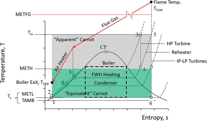
FIGURE 1. Temperature-entropy diagram of Rankine steam cycle with reheat and feed water heating.

Even if one can design a perfect cycle with zero losses and isentropic pumps and turbines, the resulting efficiency is much less than the “Carnot Target” given by Eq. 1. (This can be easily proven by using a commercially available heat balance tool to perform the relatively straightforward calculation.) In fact, the efficiency of such a perfect cycle is equal to the efficiency of the “Equivalent Carnot” cycle defined as follows:

${\eta }_{\text{CE}}=1-\frac{\text{METL}}{\text{METH}}.(2)$

where METH is the cycle’s “mean-effective heat addition temperature” and METL is the cycle’s “mean-effective heat rejection temperature”. Using basic thermodynamic relationships, one can show that METH and METL are logarithmic means of the initial and final temperatures of their respective heat transfer processes³. By virtue of the constant pressure-temperature heat rejection process via condensation, Rankine cycle METL is indeed equal to the real temperature T_L. However, METH is a hypothetical temperature, which, for a hypothetical isothermal heat addition process between states eight and five in Figure 1, results in the same amount of heat addition, which is the sum total of nonisothermal main and reheat heat addition processes. For calculation of METH in conventional steam (Rankine) cycles, refer to Gülen (2017a).

The ratio of the equivalent and apparent Carnot efficiencies defines the Cycle Factor (CF), which is a measure of the deviation of cycle heat transfer processes, either or both, from the isothermal ideal. For the purpose of generality, it is preferable to use a standard temperature for T_L and the logical choice is the ISO ambient temperature of 15°C. This convention eliminates one design specification from the discussion/analysis, i.e., the condenser pressure (steam turbine backpressure), which is highly dependent on site conditions, project economics, and prevailing regulations. Typical values of CF range between 0.82 and 0.87; assuming CF = 0.85 is sufficiently accurate for most practical purposes.

Let us open a parenthesis here. The analysis above was exclusively based on the steam cycle and steam temperatures. Also shown in Figure 1 are three “gas” temperatures: burner flame temperature, T_FLM, boiler flue gas exit temperature, T_FGX, and mean-effective average of the two, METFG. Typical flame temperature is around 2,000°C (3,600°F). Flue gas temperature upstream of the AQCS⁴ is around 130°C (266°F). Logarithmic mean of these two temperatures is 808°C. Rewriting Eqs 1, 2 with T_FLM, METFG, and T_AMB, Carnot efficiencies and CF are recalculated as

${\eta }_C=1-\frac{{\text{T}}_{\text{AMB}}}{{\text{T}}_{\text{FLM}}}=1-\frac{288}{2000+273}=87.3\%,$

${\eta }_{\text{CE}}=1-\frac{{\text{T}}_{\text{AMB}}}{\text{METFG}}=1-\frac{288}{808+273}=73.4\%,$

$\text{CF}=73\text{.}4/87\text{.}3=\text{0}\text{.}84\text{.}$

One would argue that this is the “true” measure of the steam cycle’s thermodynamic potential and the “true” T_H is T_FLM. This argument is fundamentally correct. However, for the high-level thermodynamic analysis described herein, burner flame and gas exit temperatures are not readily available numbers. Obtaining these numbers requires in-depth boiler thermodynamic and heat transfer analysis. This involves not only the heat transfer between hot combustion gas from the furnace and the heater coils (i.e., evaporator, superheaters and reheaters) but also heat recovery via combustion air heating (to increase the boiler efficiency), flue gas recirculation, etc. (See Chapters 4 and 22 in Steam (2015) for detailed boiler combustion calculations.) For the second law analysis, it is easier to omit this tedious exercise and take care of it later using a boiler efficiency (typically, 0.90–0.95) in the first law roll-up of efficiencies. We can now close the parenthesis.

The ratio of the thermal efficiency of the actual steam cycle with myriad losses (e.g., heat and pressure losses in pipes and valves, turbine expansion efficiency, etc.) to that of its Carnot equivalent is the Technology Factor (TF). Today’s state-of-the-art in SC and USC design can achieve a TF of 0.80–0.85 at METH range of 670–675 K (steam cycle only, i.e., steam turbine generator (STG) output minus boiler condensate/feed pump motor input, excluding boiler efficiency and other plant auxiliary loads). For quick estimates, one can assume that each 30 K in METH is worth 0.01 (equivalent to 1% point) in TF. Modern utility boiler LHV efficiencies are in low to mid-90s (percent). Plant auxiliary load is largely a function of heat rejection system and AQCS. Both systems are highly dependent on existing environmental regulations and permits. Optimistic values are 5–6% of STG output but can be higher. Electric motor-drive boiler condensate and feed pumps consume about 3–4% of STG output. In some designs, the large boiler feed pump (BFP) is driven by a mechanical drive steam turbine (in a steam power plant rated at 600 MWe, the BFP consumes more than 20 MWe). This reduces electric motor power, but steam extracted to run the BFP steam turbine reduces STG output; i.e., the bottom line in terms of plant thermal performance is not affected much. Going with the example above, assuming that TF is 0.82, boiler efficiency is 92%, and remaining “house load” and transformer losses constitute 2% of gross output, conventional steam plant efficiencies (net LHV) become

${\eta }_{\text{cycle}}=0.82\times 0.571=0.468\text{or}46.8\%;$

${\eta }_{\text{gross}}=\text{0}\text{.}92\times \text{0}\text{.}468=\text{0}\text{.}431\text{or}43\text{.}1\%\text{;}$

${\eta }_{\text{net}}=\text{0}\text{.}431\times \left(1-0.02\right)=\text{0}\text{.}422\text{or}42\text{.}2\%\text{.}$

For the entire plant, TF_net is 0.422/0.571 = 0.74 and the product of TF and CF is 0.74 × 0.855 = 0.63, which can be considered an overall “Carnot Factor” of conventional steam cycle technology on a net plant efficiency basis. On a cycle-only basis, state-of the-art “Carnot Factor” range is (0.80–0.85) × 0.855 = 0.68 to 0.73. The second law analysis presented above is summarized in Table 1 for quick reference. Starting point is fuel exergy (see Kotas (2012) for more on this rather ill-defined aspect of thermal bookkeeping) and ending point is net plant output at transformer high voltage terminals.

TABLE 1

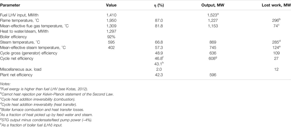
TABLE 1. Steam cycle analysis.

Which Efficiency?

When it comes to defining a cycle efficiency for a real machine, precise definitions become of utmost importance. There is no ambiguity about the definition of the denominator of the efficiency formula, which is a simple ratio⁵; it is the rate of fuel burn in the boiler, either in LHV or in HHV⁶. Since fuel is purchased on an HHV basis, industry convention in the USA has always been to quote the plant efficiencies in HHV (in Europe and Japan, LHV is preferred). Herein, the LHV benchmark is adopted as well (which results in a higher efficiency number—HHV can be higher than LHV by up to 10%) because there is practically no value to the additional heat content from a power generation perspective. The differences in efficiency definitions arise from the numerator of the efficiency formula, which are enumerated below:

1 ‐Generator gross efficiency (sometimes just gross efficiency)—based on STG output at the generator terminals

2 ‐Generator net efficiency—based on STG output minus power consumed by all cycle pumps (typically, on the 4 kV bus), which can be identified on the Rankine cycle T-s or heat and mass balance (HMB) diagram

3 ‐Plant net efficiency—based on STG output minus “house load”

4 (including heat rejection system pumps, fans, etc.) minus transformer losses.

From a practical perspective, the key performance metric is the last one—after all, this is the raison d’être of the whole enterprise, i.e., net electric power supply to the electricity network (the grid). That number is highly dependent on (1) site ambient conditions (i.e., geographical location), (2) project financing criteria and prevailing economic conditions, and (3) environmental and other regulatory requirements in force (for permitting). If one is willing to make a clear separation between fossil boiler and steam turbine technologies (including the synchronous ac generator), then the Rankine cycle efficiency is the metric that quantifies the status of the technology “on paper”, which is found from generator net efficiency divided by the boiler efficiency. It is, however, more of an academic construct rather than a number relevant to the bottom line of plant owner/operator.

Combined Cycle

The Rankine cycle analysis above is repeated for the gas turbine Brayton cycle and Brayton-Rankine combined cycle (see Figure 2). Due to their relative positions in the T-s diagram, the former is also referred to as the “topping” cycle whereas the latter is (not surprisingly) the “bottoming” cycle. Following the standard cycle notation in the figure, for the Brayton cycle one can find that

$\text{METH}=\frac{T_3-T_2}{\ln \left(T_3/T_2\right)},(3)$

$\text{METL}=\frac{T_4-T_1}{\ln \left(T_4/T_1\right)}.(4)$

FIGURE 2

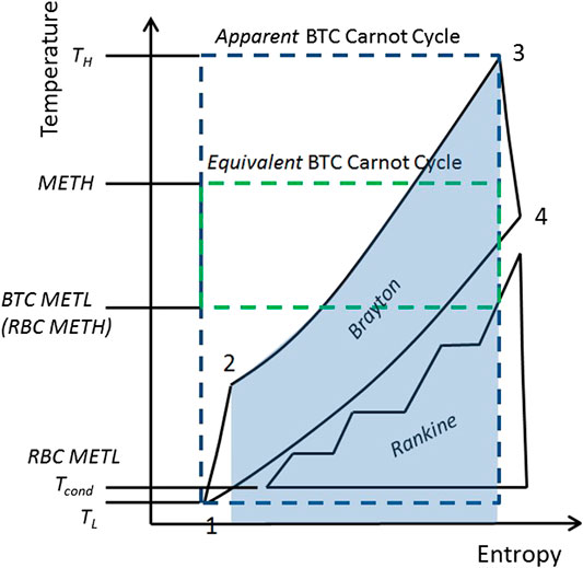
FIGURE 2. Temperature-entropy diagram of Brayton-Rankine combined cycle.

Note that the METL for the Brayton topping cycle of a GTCC given by Eq. 4 is the METH for the Rankine bottoming cycle (RBC) of the GTCC. Thus, the equivalent Carnot efficiency for the RBC is

${\eta }_{\text{CE,RBC}}=1-\frac{T_1}{\text{METL}}.(5)$

Strictly speaking, mean-effective heat rejection temperature for the RBC is the saturated steam temperature in the condenser. The implicit assumption in Eq. 5 is that the condenser loss is a part of the cycle factor, CF. Rankine bottoming cycle TF evolution is shown in Figure 3. Data plotted in the chart is culled from steam turbine OEM ratings published in Gas Turbine World and Turbomachinery International handbooks. Technology factor is calculated as

$\text{TF}=\frac{\text{STGn}\left(1-\varphi \right)}{\text{MEXH}\left(0.001628\text{n}{\text{TEXH}}^{1.60877}\right)\text{·}1.05506},(6)$

where STG is steam turbine generator output, ϕ is the feed pump power as a fraction of STG (assumed 1.9%), MEXH is gas turbine exhaust gas flow rate (lb/s), and TEXH is exhaust gas temperature (°F). STG, MEXH, and TEXH correspond to OEM rating data published in the handbooks. Thus, the denominator is gas turbine exhaust gas exergy in kW. The trend clearly points to the increasingly incremental nature of recent and possible future advances, which, by the way, come at significantly higher installed cost. Interestingly (but probably not so surprisingly), state-of-the-art Rankine bottoming (steam) cycle TF is pretty much identical to that of state-of-the-art conventional steam plant TF_net. This is a clear evidence of isothermal heat rejection and the technology built into the steam turbine will be discussed later.

FIGURE 3

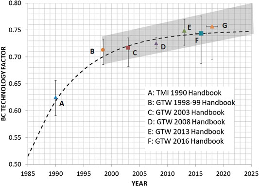
FIGURE 3. GTCC Rankine (see) bottoming cycle evolution, 1985–2018. Data points are averages; error bars denote the range (min-max) in published numbers.

For the GTCC with no supplementary firing in the HRSG, using the first law of thermodynamics, one can write the net thermal efficiency as⁷

${\eta }_{\text{CC,net}}=\left[{\eta }_{\text{GT}}+\left(1-{\eta }_{\text{GT}}\right)\cdot {\eta }_{\text{HRSG}}\cdot {\eta }_{\text{ST}}\right]\cdot \left(1-\alpha \right).(7)$

In Eq. 7, η_GT is the gas turbine efficiency, η_ST is the steam turbine efficiency⁸ (take note: not the steam “cycle”), and η_HRSG is the HRSG effectiveness, i.e., percentage of gas turbine exhaust gas energy utilized in steam production. Gas turbine and steam turbine efficiencies are inclusive of respective generator electrical and mechanical losses as well as shaft mechanical losses (e.g., bearing friction). Thus, the term in square parentheses on the right-hand side of Eq. 7 is the generator or “gross” output of the GTCC. Plant auxiliary loads (e.g., power consumed by feed pump, cooling water circ pump, and other motor-driven equipment as well as miscellaneous users such HVAC⁹ and lighting) are accounted for by α. For rating performance purposes with an open-loop water-cooled condenser and most optimistic assumptions, a good value for α is 1.6%. In the field, especially with cooling towers or air-cooled condensers and permit-driven accessory systems such as ZLD¹⁰ and gas turbine inlet chillers, α can be as high as 3% or maybe more.

For given gas turbine exhaust temperature, η_HRSG dictates the HRSG stack gas temperature. One key takeaway from Eq. 7 is the “tug of war” between HRSG effectiveness and the ST efficiency; the product of the two gives the overall RBC efficiency, i.e.,

${\eta }_{\text{RBC}}={\eta }_{\text{HRSG}}\cdot {\eta }_{\text{ST}}.(8)$

For optimal bottoming steam (Rankine) cycle design, both terms on the right-hand-side of Eq. 8 should be balanced carefully. This can be readily illustrated by the trade-off in a single-pressure bottoming cycle (see Chapter 6 in Gülen (2019b) for an in-depth discussion). Best HRSG effectiveness requires lowest possible steam pressure (or, equivalently, lowest stack gas temperature), which, of course, severely hurts the steam cycle efficiency (i.e., low main steam exergy). Similarly, best steam cycle efficiency requires highest possible steam pressure (i.e., high main steam exergy), which is detrimental to the HRSG effectiveness (i.e., high stack temperature). Optimal design point balances the two at a particular steam pressure¹¹.

Present state-of-the-art in HRSG design with modern gas turbines is three-pressure, reheat (3PRH) with high steam temperatures and pressures. 3PRH HRSG effectiveness is about 90–92% (corresponding to stack gas temperature of about 80°C). A cheaper and slightly less effective (by about 2%) variant is two-pressure, reheat (2PRH). The HRSG effectiveness is defined as

${\eta }_{\text{HRSG}}=\frac{h_{\text{exh}}-h_{\text{stck}}}{h_{\text{exh}}},(9)$

where subscripts _exh and _stck denote exhaust and stack gas enthalpies, respectively. In an earlier article, Gülen et al. (2017b) showed that, at natural gas prices prevailing in the United States, 3PRH is not an economic choice (i.e., 2PRH design would result in a lower LCOE¹²). Noting that even an infinitely large HRSG would not be able to reach 100% effectiveness as defined by Eq. 9, to expect much improvement over the current state-of-the-art is not realistic. Even a “supercritical” steam cycle is not a panacea in this respect as rigorously shown by the author in a recent study using fundamental thermodynamic arguments (Gülen, 2013).

Architecture

The steam turbine of the 750 MWe Lünen Power Plant in Germany (commissioned in 2013) is a very descriptive representative of modern technology. The steam cycle is 280/600/600 single reheat with Siemens SST5-6,000 steam turbine (four casings, HP, IP, and two double-flow LP—see Figure 4)¹³. Each LP end has an annulus area of 12.5 m². Feed water heater arrangement is HARP (Heater Above the Reheat Pressure) with nine FWHs (three HP, five LP, and one deaerating FWH) and 308°C final feed water temperature. In HARP arrangement, the last HP FWH utilizes steam from HP turbine mid-stage extraction. HARP is a key contributor to high cycle efficiency via boiler feed water entry temperature (i.e., state point 8 in Figure 1), which maximizes cycle METH. Net efficiency is 45.6% (LHV) with boiler efficiency over 94% (LHV). Estimated METH is about 690 K and η_CE is about 58.5% corresponding to a TF_net of 0.78.

FIGURE 4

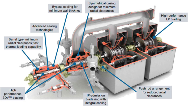
FIGURE 4. Siemens SST5-6,000 steam turbine (from Cziesla et al., 2009).

John W. Turk (JWT) in Arkansas, the United States, is the most efficient USC power plant. It is a nominal 600-MWe power plant burning PRB coal. Its steam cycle is nominally 250/600/600 (first two are main steam conditions in bara and °C and the third one is hot-reheat steam temperature in °C) and very similar to that of Lünen. Net plant heat rate is 8,730 Btu/kWh (HHV), which corresponds to 42.4% in LHV. It is worth noting that JWT steam cycle is definitely supercritical because main steam pressure (242 bar) is above the critical pressure of H₂O (217.75 bar). The cycle is, however, borderline ultrasupercritical because reheat steam temperature (607°C) is slightly above 600°C¹⁴. Due to its HARP FWH arrangement, same as that of Lünen, boiler feed water inlet temperature is 310°C, which leads to METH = 401.7°C and equivalent Carnot efficiency of 57.3%. A simplified cycle schematic is shown in Figure 5. For simplicity, the feed water heater (FWH) train with eight heaters (including a deaerating FWH) in HARP arrangement is not shown.

FIGURE 5

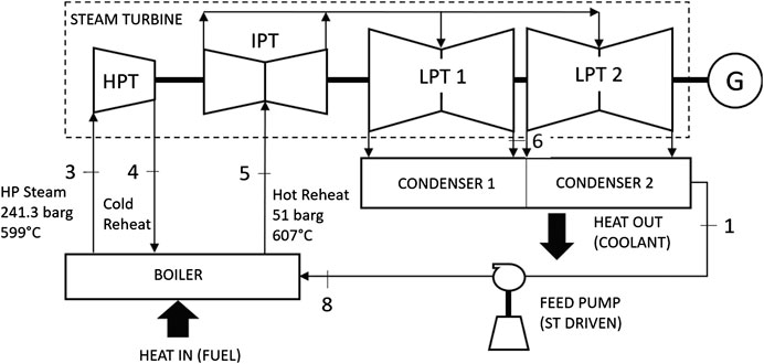
FIGURE 5. Simplified steam turbine cycle schematic.

The steam turbine in John W. Turk (JWT) power plant has four casings: one single-flow HP turbine, one double-flow IP turbine, and two double-flow LP turbines. Separate HP-IP turbines (cylinders) are necessitated by the longer expansion line of the USC cycle (higher pressure ratio from HP inlet to IP exit) so that number of stages in either turbine can be optimized separately. The OEM is Alstom Power (now owned by General Electric); it is similar in architecture to the Siemens steam turbine in Figure 4. One approach to reducing condenser pressure with the same coolant temperature is the condensers-in-series arrangement, which is widely used in twin double-flow LP configurations (i.e., four exhaust ends), which is used in JWT as well. The thermodynamic objective is the reduction of METL without excessive size and cost in heat rejection equipment. For underlying thermodynamics and a sample calculation, the reader is referred to Chapter 7 in Gülen (2019b).

The single-reheat steam turbine architecture shown in Figure 5 is the most common one with double-flow IP and LP turbines. Possible LP turbine configurations as a function of rated turbine power (i.e., steam flow) are summarized in Figure 6. Typical LSB length and corresponding exhaust area values are also provided in Figure 6. Presently, largest available annulus area is 16 m² (corresponding to about 56 in. titanium LSB length). Thus, for example, 6-flow LP arrangement with 12.5 m² annulus area (75 m² total) can be replaced with 4-flow 16 m² annulus area with little loss in performance. Combined cycle steam turbines in smaller ratings (e.g., 200 MW or less) are available in single axial exhaust LP turbine architecture. For example, instead of 2-flow 3.2 m² annulus area, single flow 6.3 m² can be used. The linear relationship between the annulus area (AAN) and LSB length (L) is quite accurately described by

$\text{AAN}\left[{\text{m}}^2\right]=\text{0}\text{.}0173\times \text{L}\left[\text{mm}\right]-8\text{.}8672\text{.}(10)$

FIGURE 6

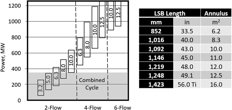
FIGURE 6. LP turbine modules for fossil power plants (numbers in rectangles denote annulus area per exhaust end in m2—1 m2 = 10.7639 ft2) and last stage bucket (LSB) lengths.

The shaft configuration in Figure 5 is commonly known as “tandem compound”. Another configuration with two shafts in parallel is known as “cross compound”, where HP and IP turbines are on a common shaft connected to a 2-pole generator at 3,000 or 3,600 RPM and the LP turbines are on a separate shaft connected to a 4-pole generator at 1,500 or 1,800 RPM (“half speed”). Cross-compounding was originally necessitated by limited availability of large generators that can absorb the total power of HP, IP, and LP turbines. Another reason for cross-compounding was very large volume flows in nuclear power plant steam turbines with low main steam inlet conditions (i.e., nearly saturated). Thus, half-speed LP shafts in those units were advantageous for very long last stage buckets without excessive centrifugal forces. Today, for all practical purposes, tandem compound single-generator designs are more economic for units rated as high as 1,100 MWe.

A steam turbine cycle/configuration variant made possible by very high main steam pressure and temperatures is double reheat. In this cycle, steam from the HP turbine goes through two (instead of one) reheat-expansion sequences. The thermodynamic principle underlying double reheat is to increase the cycle METH. This can be visually recognized easily from the cycle T-s diagram in Figure 1. Especially at high (supercritical) main steam temperatures, turbine expansion lines will shift to the left. As a result of this, the end point of IP-LP expansion will end up deeper in the two-phase zone. Higher exhaust moisture is detrimental to expansion efficiency and leads to erosion of LP last stage buckets via impact of microscopic droplets. An additional reheat step can thus bring the expansion end point back to its original place and, in addition to increasing the cycle METH, will increase LP turbine efficiency.

Interestingly enough, double-reheat A-USC technology was introduced in 1950s in the United States (Philo 6 in 1957 and Eddystone 1 in 1959). Even so, as of today, barely 40 coal-fired double-reheat units have been built globally. Most of those were built in 1960s and 1970s in Germany, the United States, and Japan. The most prominent one is Nordjylland Unit 3 in Denmark (commissioned in 1998), which is the world’s most efficient conventional steam power plant with 47% net LHV efficiency (see State-of-the-Art). Philo 6 and Eddystone 1 were retired long time ago and no USC plants, single or double reheat steam cycle, are in operation (or planned) in the United States (with the possible exception of John W. Turk). For a comprehensive summary of double reheat technology, operating plants in Germany, Japan, and China, as well as future prospects of this cycle variant, refer to the review article by Nicol (2015).

State-of-the-Art

Conventional Steam Cycle

A comparison of state-of-the-art SC Rankine, USC, and future A-USC cycle performances is provided in Table 2. For a comprehensive description of a “reference” USC coal-fired steam power plant, including the boiler, AQCS and BOP¹⁵, refer to the VGB article by Meier et al. (2004). Based on 285/600/620 steam cycle, 8 FWHs, double-flow LP with 1,400 mm (55 in.) titanium LSBs, 303.4°C feed water inlet temperature and 45 mbar condenser pressure, the projected net efficiency is 45.9% LHV in an inland location (with 0.6% (wt) low sulfur fuel to ensure low flue gas exhaust temperature). Depending on site conditions and project economics, it is claimed that 48% is possible “with certain modifications”. While the article is from 2004, it is probably a good description of the steam power plant (and steam turbine) state-of-the-art (SOA) as it exists at the time of writing (2020). (The author is not aware of an actual power plant designed, constructed, and commissioned and in operation as described in the article.)

TABLE 2

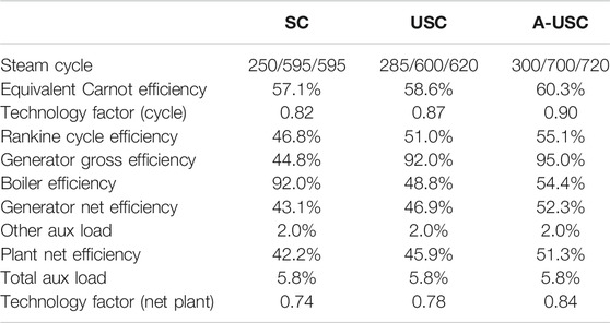
TABLE 2. Conventional steam Rankine cycle power plant efficiency roll-up.

Performances in Table 2 are still “on paper” so that it behooves us to look at the current state-of-the-art as measured in the field as well. The most efficient steam turbine power plant in the world is Vattenfall’s Nordjylland Power Station Unit 3 in Denmark rated at 400 MWe (commissioned in 1998). It is based on a double-reheat cycle with 290 bara, 582°C main steam, and 580°C (292/582/580 in short) hot reheat steam conditions. Condenser vacuum is 70 mbar with cold seawater cooling in an open loop. Net efficiency is 47% (LHV). Estimated METH is about 700 K and η_CE is about 58.9% corresponding to a TF_net of 0.80.

Another “world’s most efficient coal-fired power plant claim” was made by the OEM of the 1,050 MWe cross-compound steam turbine (250/600/610 single reheat steam cycle) in Electric Power Development Co.’s Tachibana-wan Unit 2 in Shikoku, Japan. The unit was commissioned in December 2000. Reported world record efficiency was 49% “gross LHV” at generator terminals and rated conditions¹⁶. While the cited efficiency is certainly impressive, notwithstanding the OEM claim, it is hard to see that the net thermal efficiency of this power plant can be higher than that of Nordjylland Unit 3.

600 MWe Isogo Unit 2 in Yokohama, Japan (commissioned in 2009), is based on a 250/600/620 single reheat cycle and rated at about 45% gross LHV (about 43% net). (The steam turbine is supplied by Siemens.) This performance is similar to that of several German USC power plants, e.g., RWE Power’s Neurath units F and G (also referred to as BoA 2 and 3, respectively¹⁷), each rated at 1,100 MWe with over 43% net LHV efficiency. The steam cycle is 270/600/600 with 48 mbar condenser pressure (natural draft cooling tower providing 18.2°C circulating water), which suggests a TF_net of 0.73–0.74.

Bottoming Steam Cycle

Based on the published performance data of 1,700°C TIT class “super heavy-duty” gas turbines (from Gas Turbine World’s 2020 Handbook—the primary trade publication with budgetary price and performance data for simple and combined cycle gas turbines), the current state-of-the-art in Rankine (steam) bottoming cycle can be summarized as follows:

1 ‐Equivalent Carnot efficiency, η_CE,RBC of 48.2% ± 0.5%

2 ‐HRSG effectiveness, η_HRSG of 92.3% ± 0.4%

3 ‐Steam turbine efficiency, η_ST of 41.5% ± 0.3%

4 ‐Bottoming cycle efficiency, η_RBC of 38.3% ± 0.4%

5 ‐Technology factor (gross) of 79.4% ± 0.2%.

It was already pointed out (see Figure 3 and the accompanying discussion) that modern Rankine bottoming cycle TF is comparable to that of the modern conventional SC or USC steam power plant (based on net plant output). A side-by-side comparison of two state-of-the-art steam cycles is presented in Table 3. The conventional steam cycle is based on JWT described in Architecture. Bottoming steam cycle, as noted earlier, is based on the typical rating performance with a 1,700°C class advanced gas turbine. While the comparison is not truly “apples to apples”, both are representative of the current state-of-the-art in steam turbine technology.

TABLE 3

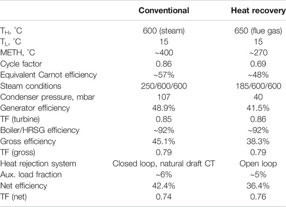
TABLE 3. Comparison of conventional and heat recovery steam cycle performances.

Bottoming cycle CF is lower than the CF for conventional steam power cycle. The reason is directly tied to the high value of feed water temperature entering the fossil fuel boiler (via feed water heating with steam extraction from the turbine), which increases the METH of the conventional steam cycle vis-à-vis that of the Rankine bottoming cycle. Prima facie, the question that arises is this: Why do not we use feed water heating in the combined cycle steam turbines as well to raise METH? The answer is that feed water heating is highly detrimental to bottoming cycle performance because it raises the HRSG stack gas temperature and hampers the heat recovery effectiveness.

Future of the Art

The quantitative picture depicted in Table 3 strongly attests to the fact that steam turbine technology has reached a plateau. This is the end result of sustained engineering achievements over the course of the last century. Let us repeat: a TF value of 1.0 implies that the system in question is effectively a “Carnot engine”. Yet, in terms of STG output at the low-voltage terminals of the step-up transformer, at a value of 0.85, current technology comes within a proverbial inch of that theoretical upper limit. Subtracting power consumption of cycle pumps, this number comes down to 0.82. Remaining deductions are (1) losses in the heat transfer equipment (i.e., fossil boiler or HRSG), (2) power consumed by the BOP equipment, especially the heat rejection system, and (3) the “house” load. As discussed earlier, at state-of-the-art efficiency/effectiveness levels in low to mid 90s, there is not much room left in boiler/HRSG technology for any meaningful gain. In fossil boilers, 95% LHV is probably the practical limit, which has already been achieved in the field (e.g., 94.4% in lignite-fired Niederaußem in Germany). In HRSGs, the practical limit is probably 92% in state-of-the-art 3PRH systems with advanced class gas turbines. In either case, further improvement is unlikely—if nothing else due to limits imposed on flue gas exit temperature based on corrosion (condensation of H₂O) and/or plume abatement considerations (stack effect). On top of it all, any small gains are guaranteed to come at exorbitant cost to render them infeasible (unless, of course, fuel prices are exorbitant, too). The same is true for the balance of plant (BOP) equipment (i.e., pumps, fans, AQCS, etc.) as well. In fact, due to stringent environmental regulations making water-cooled steam condenser heat rejection systems practically impossible, even higher plant auxiliary loads are to be expected. Consider that net retirement of 4,000 MWe of once-through cooling steam generation was cited as one of the key contributors to recent power outages in California (on August 14, 2020, while these lines were being written).

Conventional Steam Cycle

The first question is obvious: Where are the steam cycle losses and how big are they? In order to answer this question, let us look at the conventional steam cycle in Table 3. Using the equivalent Carnot efficiency of 57.3% as the starting point, the “stairsteps” to the actual generator efficiency are listed in Table 4 (also included for reference are the stairsteps starting from the actual generator (gross) efficiency). The “other losses” step includes steam leaks, pressure losses in steam lines (including reheater and crossover pressure drops) and heat exchangers, steam turbine valve pressure drops, mechanical (bearing friction) losses, and irreversibility in feed water heaters.

TABLE 4

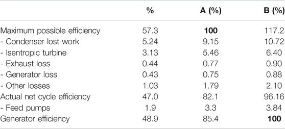
TABLE 4. Steam turbine/cycle efficiency breakdown (column A: reference to maximum possible efficiency, column B: reference to generator (gross) efficiency.

Table 4 clearly shows that there are two major deviations from the thermodynamic ideal: lost work due to heat rejection across a finite temperature difference and nonisentropic expansion of steam in the turbine flow path. Exhaust and generator losses are relatively minor and do not present any significant improvement opportunities¹⁸. It is also unrealistic to expect much from reduced pressure losses and feed water irreversibilities.

Individual turbine efficiencies for the JWT (using a heat and mass balance model to match the reported data) are summarized in Table 5. Turbine stage inefficiencies stemming from leaks, boundary layer growth (profile and secondary flow) losses, moisture or wetness losses, aerodynamic effects, e.g., wake mixing (transonic) and shock dissipation losses (supersonic), tip leakage losses, etc. can certainly be reduced by 3D aero design utilizing advanced CFD, machine learning, and other new computational and manufacturing technologies (i.e., 3D printing of complex parts). The question is, of course, how close one will get to the isentropic ideal. Vintage turbine designs (before ca. 1990) used either pure impulse (also known as diaphragm-wheel) or 50% reaction designs. In the former, enthalpy drop takes places fully across the nozzle vanes, which convert the thermal energy into kinetic energy. Consequently, rotor blades are similar to hydraulic turbine “buckets”; i.e., blade cross-section is like a symmetrical crescent¹⁹. Torque is created by imparting momentum on the buckets. Due to the different shapes of vanes and buckets and large flow deflection across the buckets, profile and secondary losses are high leading to lower stage efficiency. On the plus side, the impulse design is amenable to higher stage loading and, for a given pressure drop, it requires fewer stages (e.g., 5 or 6 HP turbine stages). In reaction design, enthalpy drop is distributed between stator vanes and rotor blades, e.g., equally in 50% reaction design. Thus, vane and blade shapes (and velocity triangles) are identical so that, in addition to smaller flow deflection, they lead to lower profile and secondary losses and higher stage efficiencies. On the minus side, stage loading in reaction design is limited and, for a given pressure drop, roughly twice the number of impulse stages is necessary in a reaction design. Furthermore, due to the axial thrust on the rotor created by the pressure difference across the blades, a dummy balance piston is required in single flow designs (i.e., the HP turbine mainly). The leakage across the balance piston reduces the turbine efficiency.

TABLE 5

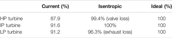
TABLE 5. Steam turbine efficiency summary.

Modern practice is to design the steam path with 3D Navier–Stokes solvers combined with numerical optimization algorithms to determine the optimal reaction for each turbine stage. The optimization process determines stage reaction from the inlet (low reaction, high loading) to the exit (high reaction, low loading) while accounting for the variation in velocity triangles from the blade root to the blade tip. This results in twisted blade shapes (high aspect ratio, long blades with “aft-loaded” profiles). In some modern designs, all blades in HP and IP turbines are integrally shrouded with optimized labyrinth-type seals to minimize leakage losses. (Shaft leakage losses are minimized by replacing traditional labyrinth seals by brush seals, abradable coatings, and spring-backed seal segments.) Another modern innovation is “bowed” or “leaned” stator blades to reduce secondary losses. For a comprehensive description of the 3D design practices by different OEMs, consult Jansen and Ulm (1995); Deckers and Doerwald (1997); Oeynhausen et al. (1997); Simon et al. (1997); Simon and Oeynhausen (1998), and Boss et al. (2005). The impact of all items enumerated above was estimated as 2 percentage points of improvement.

Total turbo-generator losses constitute about 7% of the theoretical maximum (e.g., see Table 3). Very little (if any) can be shaved off of valve, exhaust, and generator losses. State-of-the-art, synchronous ac generator technology is represented by Siemens SGen5-3000 W series (two-pole) generator with water-cooled stator windings, hydrogen-cooled rotor, static excitation, two-channel digital voltage regulator, and the auxiliary systems (i.e., seal oil, hydrogen and water units). These machines typically achieve over 99% efficiency.

Exhaust loss minimization requires large enough flow annulus area to bring the steam velocity to an optimum, which is typically around 700 ft/s (215 m/s). For a detailed discussion of the underlying theory and determining the economic minimum, the reader should consult Chapter 5 in Gülen (2019b) and references cited therein. In general, the higher the steam turbine rating, the higher the steam flow. Furthermore, the lower the condenser vacuum (i.e., steam turbine backpressure), the larger the requisite annulus area to maintain the optimal steam exhaust velocity with given steam flow. For a plant rated at 600 MWe and with 45 mbar condenser vacuum, the ideal design is a 4-flow LP turbine (i.e., two double-flow LP turbines) with 16 m² annulus area per end. This requires long last stage buckets (LSB), i.e., 56 in. or 1,423 mm long, made from titanium (to minimize weight without sacrificing strength, i.e., minimize centrifugal forces acting on the long blade). Such long blades have a strongly twisted profile to minimize aerodynamic losses (enabled by advanced CFD and 3D aero codes²⁰) and accommodate large deviation in tangential speeds between the blade root and tip. To reduce tip leakage losses (Mach number at the blade tip is about 2, corresponding to 750 m/s, implying a rotor diameter of about 1,900 mm) and introduce stiffness (i.e., increase dynamic stability), the blades are connected via mid-span “snubbers”²¹ and incorporate integral tip shrouds.

How much can be trimmed of the remaining 5.5% via better steam path aerodynamic design is difficult to say. Considering the very long history of steam turbine technology development, the expectation herein is not more than 1% (if that). Nevertheless, OEM-reported efficiencies for Siemens’ five-casing steam turbine in VEAG (Vereinigte Energiewerke AG—a German utility) Boxberg power plant in Germany were 94.2% (“internal” HP turbine efficiency was the term used) and 96.1% (IP turbine efficiency) (Hoffstadt, 2001). This power plant, rated at 907 MWe, has a relatively modest steam cycle (266/545/581) with 48.5% gross and 42.7% net plant efficiency (pretty much the same as JWT but with a lower METH, about 390°C)²². Due to the relatively short LSB size (39 in. length), a 6-flow LP turbine configuration (three double-flow casings) had to be adopted. Modeling the steam turbine in Thermoflow, Inc.’s THERMOFLEX software, performance reported in Hoffstadt (2001) was achieved with 60 mbar condenser pressure and turbine efficiencies listed in Table 4, which are significantly lower than reported values.

Similarly, not much can be done about condenser lost work, which is calculated in Gülen and Smith (2010) as

${\dot{W}}_{\text{lost}}={\dot{Q}}_{\text{cond}}\left(1-\frac{{\text{T}}_{\text{ambient}}}{{\text{T}}_{\text{steam}}}\right),(11)$

where T_steam is the temperature of steam condensing at the condenser pressure (107 mbar in JWT, the source of data in Table 4). Lower condenser pressure (vacuum) and steam temperature are dependent on the availability of a suitable heat sink. (Not to mention a multicasing LP turbine design with long—possibly titanium—LSBs to exploit the low backpressure without exorbitant losses, i.e., large size and cost.) In that sense, the ideal heat sink is a natural body of water (e.g., lake, river, ocean, etc.) from which cold water can be drawn and to which warm water can be returned. However, concerns about water resource scarcity and other environmental regulations have been increasing and are expected to grow in future, leading to greater deployment of dry cooling systems (mostly, air cooled condensers or A-Frame condensers) (Gülen, 2017a). Nevertheless, especially for rating purposes, steam power plant performances are quite frequently quoted with once-through (open loop) condenser and low vacuum (e.g., 1.2 in. Hg or 41 mbar). While this can add about 2.5 percentage points to net plant efficiency for “sticker performance” purposes, it is far removed from a realistic performance that can be achieved in most places with increasingly stringent environmental regulations.

The next logical place to look for improved cycle performance is the cycle itself or, more specifically, main and hot reheat steam conditions. Instead of trying to reduce cycle losses and irreversibilities, this approach seeks to increase the “theoretical potential”, i.e., equivalent Carnot efficiency via increasing METH. A financial analogy can be made as follows: one can make $100,000 annually if he or she invests (1) $1 million with 10% return rate or (2) $2 million with 5% return rate. The impact of steam cycle on net plant efficiency, as a function of METH (i.e., as a function of η_CE), is illustrated by the chart in Figure 7. There are two curves in the chart.

1 ‐The lower curve assumptions are 92% boiler efficiency, realistic heat sink similar to that in JWT power plant (i.e., about 100 mbar), 6% plant aux load.

2 ‐The upper curve assumptions are 94% boiler efficiency, 5% aux load, 1 in. Hg (34 mbar) lower condenser pressure.

FIGURE 7

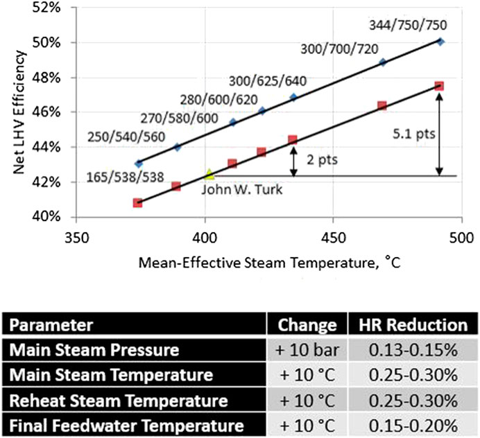
FIGURE 7. Steam cycle impact on net plant efficiency.

Cycle conditions are main steam pressure and temperature and hot reheat steam temperature in bara and °C. Performance derivatives for each parameter and final feed water temperature are listed below the chart. Note that all cycles in Figure 7 are single-reheat. Double reheat can add another 1.5 percentage point.

Higher steam pressures and temperatures demand use of alloy materials. This is illustrated in Figure 8. P91 is a ferritic alloy (9% Cr, 1% Mo) with high creep strength. P92 or NF616 [9% Cr, 2% W (tungsten)] is an improved version of P91 with higher creep strength and temperature rating (620°C vis-à-vis 593°C for P91). X20 is high-alloy CrMoV (pronounced “chromaly vee”) high-pressure steel with 12% Cr in use since early 1960s (temperature rating 565°C). NF12 is a fourth generation ferritic steel with increased content of W and Co. The ultimate goal of 700°C (1,300°F) temperature capability requires nickel-based superalloys. At 700°C and above, the cycle is referred to as advanced USC (A-USC). Major OEMs in different countries made significant R&D investment in A-USC materials supported by national or international programs such as Japan’s “Cool Earth”, European Union’s “Thermie” AD-700, and Europe’s COST²³ programs: COST501 (1986–1997), COST522 (1998–2003), and COST536 (2004–2009)—see Kjaer and Bugge (2004) and Kern et al. (2010). A summary of high temperature steels and alloys used in construction of major steam cycle components is provided in Table 6 (Zörner, 1994). For an in-depth look at supercritical power plants and the high-temperature materials enabling their performance and RAM²⁴, refer to the article by Viswanathan et al. (2004).

FIGURE 8

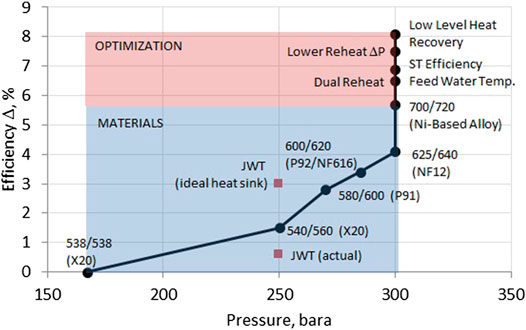
FIGURE 8. Steam turbine power plant efficiency improvement roadmap.

TABLE 6

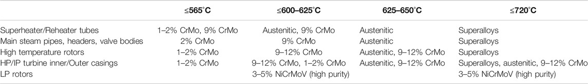
TABLE 6. Steels used for construction of high temperature steam cycle components (Zörner, 1994).

Bottoming Steam Cycle

An in-depth investigation of bottoming Rankine steam cycle loss mechanisms was done by Gülen and Smith (2010) using the second law of thermodynamics as the guide. Not surprisingly, the analysis therein showed that three mechanisms dominated the second law losses: heat recovery loss in the HRSG, steam turbine losses, and heat rejection losses. Since the analysis in the cited study is already a decade old, it is revisited using advanced class gas turbine combined cycle examples from Gas Turbine World’s 2019 Handbook. Thermoflow’s GT PRO (Version 27.0) heat and mass simulation software is used for combined cycle performance calculation. Very aggressive (i.e., expensive to procure and construct) bottoming cycle design assumptions are used to evaluate the best possible outcome with state-of-the-art technology, i.e.,

1 ‐10°F (5.6°C) pinches in HP, IP, and LP evaporators;

2 ‐180 barg/600°C/600°C steam cycle;

3 ‐once-through HP evaporator (i.e., effectively economizer approach subcool is zero);

4 ‐open-loop water-cooled condenser with OEM-listed steam pressures;

5 ‐8.5% reheater pressure loss.

Table 7 shows the efficiency values for HP, IP, and LP turbines recorded during recent tests of combined cycle steam turbines (Zachary and Koza, 2006). The efficiencies in the table are referred to as “cylinder” efficiency, which is the “total-to-total” isentropic efficiency (because kinetic energy losses are negligible) of the turbine steam path from inlet to the exit and excludes valve losses for the HP and IP turbines. For the LP turbine, cylinder efficiency accounts for the moisture loss but excludes the exhaust loss. It is the efficiency based on the expansion line end point (ELEP)—a General Electric term; see Cotton (1998) for detailed calculations. The actual turbine efficiency accounting for all losses is based on the used energy end point (UEEP). The difference between the two efficiencies is a function of steam exhaust velocity and exhaust moisture (8–10% by weight, typically). The exact formula can be found in Cotton (1998). For a rough estimate of reduction in cylinder efficiency (in percentage points) with exhaust loss, use

$\Delta \eta =3\text{.}4175\times \left(\text{VAN}/1000\right)^1\text{.}8554\text{.}(12)$

with VAN in ft/s. For an optimal design value of about 660 ft/s (∼200 m/s), Δη is 1.6 points. Steam turbine efficiencies used in the GT PRO model are in line with the data in Table 7.

TABLE 7

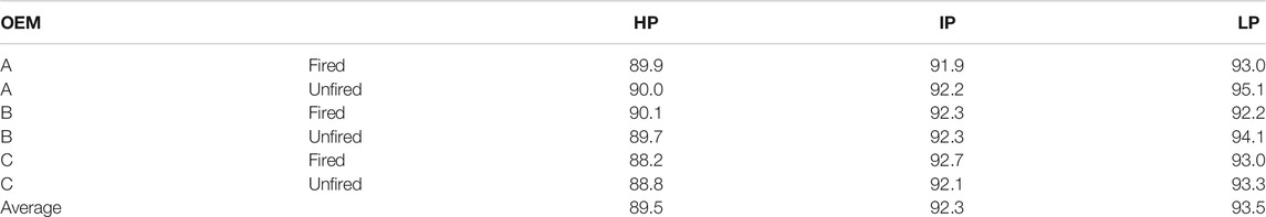
TABLE 7. GTCC steam turbine section (cylinder) efficiencies.

Calculated performance data is summarized in Table 8, which indicates that combined cycle performance (including realistic assessment of plant aux load) with 44% efficient gas turbines falls in the range of 63–64%. With a “bare bones” plant auxiliary load assumption, excluding fuel gas compressor and step-up transformer, current state-of-the-art in GTCC technology is 64% (net LHV) rating efficiency.

TABLE 8

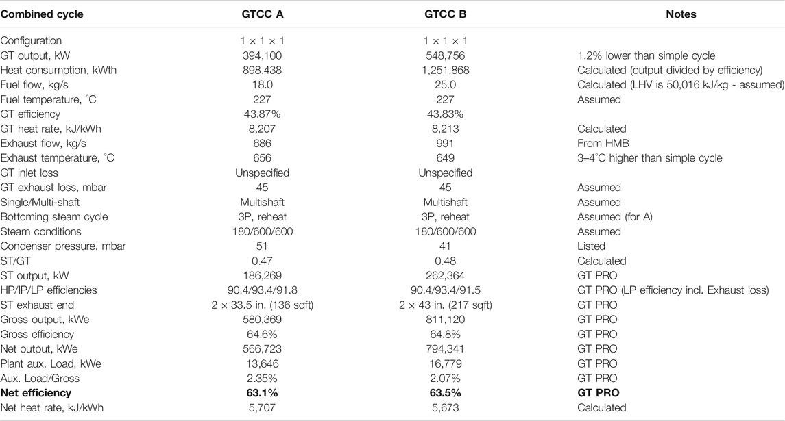
TABLE 8. Combined cycle performance estimates with advanced class gas turbines.

For comparative bottoming cycle evaluation, the best yardstick is the exergy of gas turbine exhaust gas. Using the exergy balance information generated by the GT PRO model, bottoming cycle exergy balance for GTCC A in Table 8 is summarized in Figure 9 (GTCC B exergy balance is very similar). In summary, bottoming Rankine steam cycle technology factor (based on net bottoming cycle output, i.e., STG output minus feed pump power consumption) with (1) exhaust conditions commensurate with advanced gas turbines (about 1,200°F or 650°C) and (2) aggressive design parameters is ∼0.79. This performance can be cost-effective in certain type of applications with (1) high capacity factor (e.g., at least, 6–7,000 h of operation annually), (2) high natural gas (e.g., imported LNG) prices, and (3) access to a cooling water source and lax environmental regulations. For power plants planned for cyclic operation in regions with low natural gas prices (e.g., in the United States after the shale gas “boom”), this is very unlikely to be the case.

FIGURE 9

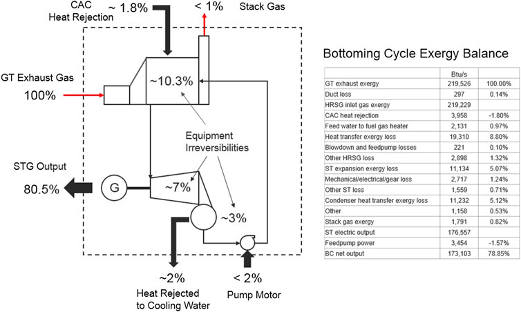
FIGURE 9. Bottoming cycle exergy balance (GTCC A)—1 Btu/s = 1.05506 kW.

As stated earlier, the data in Figure 9 dramatically illustrates the remarkable engineering achievement implicit in a state-of-the-art 3PRH Rankine steam bottoming cycle. For both OEMs, STG output is about 80% of theoretically possible maximum. It is safe to say that there is very little room left for further improvement. As far as the heat sink is concerned, for rating performances, these losses are evaluated at very low pressures with open loop water-cooled configuration. The same can be said for steam turbine losses, which are quite comparable to that for the conventional steam cycle (not surprisingly), as well as for the HRSG losses. Nevertheless, as painstakingly demonstrated by the author in recent papers, OEMs are not immune to claiming performances with a cavalier attitude toward the laws of thermodynamics (see Gülen, 2018 and Gülen, 2019c). It is difficult to predict how close the current technology is to practical entitlement. If a guess has to be made, based on the asymptotic nature of the technology development trend in Figure 3 and the calculations summarized in Figure 9 with quite optimistic assumptions, to expect a (cost-effective) technology factor above 80% is unrealistic—and, if the published ratings are to be believed, OEMs are already there!

Another Rankine Cycle

In the last decade or so, venerable steam turbine and its Rankine cycle had an emerging competitor to vie for its place in the pantheon of heat engines: supercritical CO₂ (sCO₂) cycle. It should be added that the sCO₂ technology has its Brayton cycle variant as well. In either variant, the heat engine operates in a closed cycle with CO₂ as the working fluid. The moniker “supercritical” refers to the fact that state points of the cycle are at pressures and temperatures around or significantly above the critical point of CO₂ (73.8 bar, 31°C). In their most basic embodiment, both cycles incorporate recuperation of heat from the exhaust stream of the turbine to heat the compressed working fluid from the discharge of the compressor/pump²⁵. For an in-depth critique of sCO₂ cycles, the reader is referred to a recent article by Gülen (2016). Herein the focus is on the split-flow recompression variant of the Rankine sCO₂ cycle shown in Figure 10.

FIGURE 10

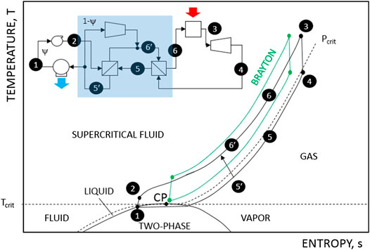
FIGURE 10. Supercritical CO₂ Rankine cycle with split-flow and recompression (turbomachinery isentropic efficiencies >90%, recuperator effectiveness >98%).

In passing, it should be emphasized that the only difference between sCO₂ Rankine and Brayton cycles in Figure 10 is in the heat rejection part of the cycles. The phase change of the working fluid from vapor to liquid is present in the low pressure region of the cycle labeled as “Rankine” but absent in the high pressure region. To be precise, the cycle should be called “half-Rankine” or “Rankine-Brayton hybrid.” Instead of this awkward phrasing, however, it is referred to as the Rankine cycle. The reader should be cognizant of the difference between the two Rankine cycles, i.e., sCO₂ and steam.

sCO₂ Standalone Power Cycle

As highlighted by the shaded rectangle in Figure 10, the single-recuperator scheme is replaced by a two-heat exchanger configuration and a second compressor, which assumes part of the preheating duty. Only a fraction ψ of the working fluid is sent through the condenser and the main cycle pump; the remaining fraction, (1 − ψ), is directed to the “recompression” or “bypass” compressor. One can easily verify that for ψ = 1.0, the split-flow cycle reverts back to the basic recuperated cycle. Due to the reduction in cycle heat rejection (ψ < 1), recuperation effectiveness and cycle thermal efficiency improve significantly. Cycle studies for similar conditions have shown that the optimal value of ψ is 0.68, which is also the value used herein²⁶.

Performance of an advanced split-flow recompression Rankine cycle with 300 bara and 760°C turbine inlet conditions is shown in Table 9 and compared to conventional steam cycle variants in Table 2. Based on the numbers in the table, at best, i.e., when the technology fully matures (if ever), sCO₂ Rankine cycle can indeed match or exceed USC or A-USC steam Rankine cycle efficiency, which has at least a century of head start in development and, more importantly, in millions of hours of field operation experience. The driver of this advantage is high cycle factor (CF) as a result of high cycle METH. The difference is due to the respective “boiler” inlet temperatures of the working fluids. In the case of steam boiler, it is the feed water temperature around 300°C, which is achieved via steam extraction from the turbine to heat the condensate successively in feed water heaters. In the case of the sCO₂ cycle, it is the temperature of the working fluid at the main heat exchanger inlet, well above 500°C, which is achieved via recuperation using turbine exhaust stream. However, in terms of net plant thermal efficiency, due to the poor fired heat exchanger effectiveness (less than 80%), sCO₂ cycle cannot compete with steam Rankine cycle in fossil fuel-fired applications (where boiler efficiency can be as high as 95%).

TABLE 9

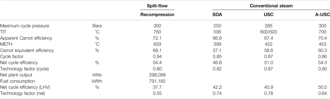
TABLE 9. Supercritical CO₂ Brayton and Rankine cycles with recuperation.

sCO₂ Bottoming Cycle

Let us look at various sCO₂ cycle performances from a GTCC bottoming cycle perspective. The topping cycle is based on a nominal 340 MWe advanced class gas turbine with about 640°C exhaust temperature and 686 kg/s exhaust flow (∼41% net LHV). Turbine inlet temperature of the sCO₂ cycles is assumed to be 600°C commensurate with the gas turbine exhaust gas temperature. Since the objective is to achieve highest possible CC efficiency, one more sCO2 cycle variant is added to the list of cases to investigate the trade-off between heat recovery effectiveness and thermal efficiency of the bottoming cycle. This is also a split-flow arrangement with a cascaded turbine (no recompression) as shown in Figure 11. The results are summarized in Table 10, which clearly demonstrates that sCO2 falls significantly short of steam in a bottoming cycle role.

FIGURE 11

FIGURE 11. Supercritical CO₂ Rankine cycle with split-flow and cascaded turbine.

TABLE 10

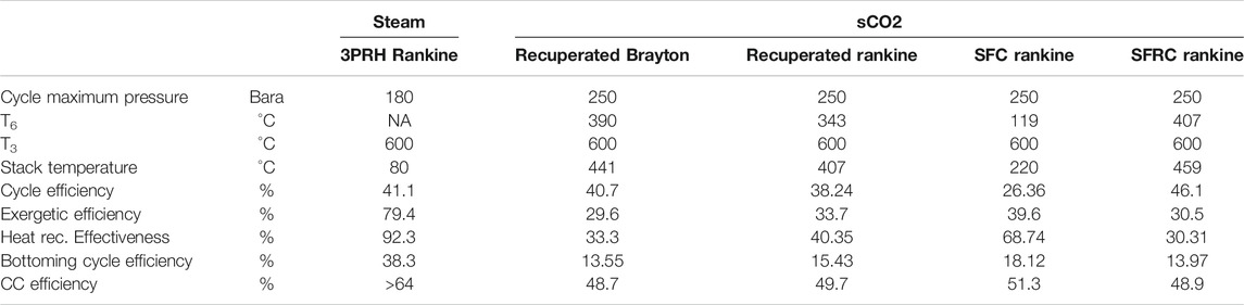
TABLE 10. Steam and sCO₂ bottoming cycles with advanced gas turbines (SFC: Split-Flow Cascaded, SFRC: Split-Flow Recompression). Combined cycle efficiency accounts for cycle pumps (including circ water pump) but no other aux load.

As the cases in Table 10 clearly demonstrate, when it comes to bottoming cycle design, thermal efficiency is only a part of the puzzle. Equally important, maybe more so, is the extent of heat recovery as quantified by the heat recovery effectiveness. This can be verified by examining the basic CC efficiency formula, Eq. 7, repeated below sans auxiliary load, i.e.,

${\eta }_{\text{CC,gross}}={\eta }_{\text{GT}}+\left(1-{\eta }_{\text{GT}}\right)\cdot {\eta }_{\text{HRSG}}\cdot {\eta }_{\text{ST}}.(13)$

The term in the parentheses on the right-hand-side of Eq. 13 is roughly equal to the GT exhaust energy. The heat recovery effectiveness, η_HRSG, is 100% if one could cool the exhaust gas down to the zero enthalpy level (an impossibility in a real system as discussed earlier). Today’s state-of-the-art 3PRH heat recovery steam generators (HRSG) with H and J class turbines can easily go beyond 90%. The thermal efficiency, η_ST, is the STG output divided by the cycle heat input, which is the product of GT exhaust energy and HRSG effectiveness. Modern steam turbines in 3PRH bottoming cycles are typically 41–42% under the most favorable circumstances. Thus, the overall bottoming cycle efficiency given by Eq. 8, repeated below for convenience,

${\eta }_{\text{RBC}}={\eta }_{\text{HRSG}}\cdot {\eta }_{\text{ST}},$

is around 36–38% for today’s super-efficient H/J class-based combined cycles (35–37% on a net basis after subtracting all the auxiliary loads).

From the numbers in Table 10 it can be deduced that

1 ‐sCO₂ Brayton cycle is less suited to be a bottoming cycle (vis-à-vis the Rankine cycle) because it limits the heat recovery due to its high temperature state-point 2. (Note that, cascaded or split-flow variants of the Brayton cycle are not included in the table. They show similar improvement but are not as good as their Rankine counterparts.)

2 ‐In terms of first law (thermal) efficiency, sCO₂ Rankine cycle with split-flow recompression is superior to even the crème de la crème of GTCC steam turbines. However, since that performance comes at the expense of heat recovery effectiveness, it is not a good candidate for GTCC bottoming cycle. (Even the more modest simple recuperated cycle has a quite respectable 38% thermal efficiency but better bottoming cycle efficiency.)

3 ‐Conversely, sCO₂ split-flow cascaded-turbine Rankine cycle has relatively poor thermal efficiency but it more than makes up for it via improved heat recovery effectiveness. As such, in terms of overall bottoming cycle efficiency, it is the best of the bunch.

Operability

In the past, conventional steam turbine power plants, coal-fired and nuclear, were the base load workhorses of the power grid. They were rarely shut down and operated at very high capacity factors. The same could be said of the early CC power plants. In fact, in the 1990s, F class gas turbine CC power plants were designed for base load duty and operated as such. With increasing penetration of renewable technologies, primarily solar and wind, into the generation portfolio in 2000s, however, all fossil fuel-fired power plants were required to cycle more than before. The reason is the inability of solar or wind resources to be dispatched on demand. They operate at low capacity factors because they are dependent on prevailing weather conditions. If there is a demand for power but there is not enough sunshine or wind, dispatchable fossil fuel resources are required to take up the slack. Some of those instances can be planned, e.g., at night when solar power generation is inactive. In those cases, operators can plan their plant startup beforehand to prevent wear-and-tear of equipment due to thermal stresses and/or shocks. In other instances, the need can arise unexpectedly, e.g., when there is a sudden drop in wind or cloud cover at a time when there is high demand for power. In that case, the sudden drop in power supply should be made up by rapidly responding resources, either starting from “cold iron” or ramping to full load from a low-load state (“spinning reserve”). For the latter type of response, the fossil fuel resource must be able to operate reliably and efficiently at a low load in compliance with emissions requirements.

Due to the design complexities of large fossil boilers and AQCS equipment, thick-walled steam pipes and valves and large metal mass associated with the steam turbine casings and rotor, steam power plants are difficult to adapt to cyclic and low load operation. Typically, large steam plants can turn down to 40–50% load with about 4–6% increase in heat rate. The exact value depends on the boiler, steam turbine, BOP, and AQCS equipment characteristics. Typically, lignite fired power plants have more limited turndown capability (i.e., higher minimum load than hard coal-fired plants). Whether fired with hard coals (bituminous) or lignite, existing plants can be retrofitted with technologies such as indirect firing, coal mill switch (from two parallel units to one unit), control system upgrades (i.e., instead of fixed “schedule” based controls with large built-in margins, a model-based “adaptive” or “dynamic” control philosophy), auxiliary firing with dried lignite ignition burner, and other features—see Henderson (2014) and IRENA (2019).

For modern SC power plants, maximum ramping rate is about 7–8% per minute from 50% to 100% load. This is significantly better than the performances of vintage SC power plants recorded by EPRI in a 1982 survey (about 2–4.3% maximum, about 1% on average) (Henderson, 2014). In existing (and old) power plants, fast response can be achieved by running the power plant with throttled steam admission valve. When additional power is needed, the valve is opened to allow more steam to flow and generate more power. (Typically, a spinning reserve equivalent to 2.5% of the rated output is possible with 5% throttling.) This is not an ideal solution because the plant operates at low efficiency before and after the valve opening. Another less-than-ideal method is to close the steam extraction valves between HP and LP turbines and respective FWHs. This increases generator output via higher steam flow through the turbine at the expense of efficiency due to lower feed water temperature at the boiler inlet.

Similar operational features can be and are adopted by GTCC power plants as well. Running the steam turbine (normally operating in a “valves wide open” or VWO mode) with throttled main steam stop-control valve (SCV) is an option for fast frequency response as required by the applicable grid code. At a grid underfrequency event, SCV is rapidly opened so that energy bottled in the HRSG is released for an extra power “shot” from the STG as a “primary” response (say, within 10–15 s). Due to its much faster dynamic characteristics, the primary response is easier to obtain from the gas turbine via overfire (with some sacrifice in hot gas path component life—as specified by the OEM), opening of the inlet guide vanes (IGVs) or even activation of compressor on-line wash sprays (extra mass through the machine). This would contribute to a “secondary” response from the steam turbine as well, but it is slower in kicking in due to the large thermal inertia of the HRSG. In order not to exceed the maximum allowable main steam pressure specified by the OEM, the steam turbine can be equipped with an “overload” valve, which would open and redirect some of the main (HP) steam into a downstream stage in the HP turbine.

Steam turbine stress control and concomitant control actions (e.g., cascaded steam bypass and terminal attemperators during startup, prevention of HP turbine heating during turbine roll to FSNL via windage heating, transition to HP turbine steam admission, prevention of LP turbine windage heating, etc.) are well known and widely implemented by major OEMs in the field. Further refinements to shave off extra minutes from startup time can certainly be achieved by exercising sophisticated dynamic simulation models in conjunction with 3D CFD analysis (a steam turbine “digital twin” maybe) to account for thermal stresses across the rather complex rotor geometry²⁷. Welded rotors made from materials suitable to each turbine section’s operating steam conditions (up to 40% lower thermal stresses during transients vis-à-vis monobloc rotors at the same steam conditions), HP turbine inner casing shrink-ring design for radial symmetry, optimization of shaft seals (e.g., advanced clearance control (ACC) with spring-loaded seals), bearing configuration (e.g., how many thrust bearings, where to put them, etc.), and other mechanical refinements (e.g., HP turbine exhaust end “evacuation” line) are also investigated and implemented by major OEMs (e.g., see Saito et al., 2017).

As far as future trends are concerned, one can point to the ever larger size of “super heavy duty” H/J class gas turbines with more than 500 + MWe output (50 Hz) in simple cycle. A 2 × 2×1 GTCC with one of these machines would be rated at 1.5 GWe with a 500 + MWe steam turbine. This brings the size of combined cycle STGs into the same league as coal-fired boiler-turbines, i.e., conventional steam plants. The ramification of this trend is increasing bucket sizes, not only in the LP turbine, which can be somewhat controlled by increasing the number of LP exhaust ends—at extra installed cost of course—but also in the IP turbine. Protecting windage heating in IP and LP turbine creates a tug of war between steam flow required to roll the unit (e.g., via IP turbine steam admission) and steam flow required to keep the long last stage buckets “cool”. This is so because controlled acceleration from turning gear (a few RPMs) to FSNL (3,000 or 3,600 RPM) requires precise control of steam flow, which may not be enough for overheating protection. This is especially true if the steam turbine is rolled to FSNL via HP steam admission. Accomplishment of this balance puts a big onus on the admission as well as bypass valves and precise control schemes.

Thermal stress and temperature ramp rate considerations become increasingly limiting as steam conditions rise to SC (for GTCC), USC, and ultimately A-USC (for conventional fossil fuel-fired steam power plants). At those demanding conditions with temperatures above 600°C turbine, steam pipe and steam valve construction materials transition from ferritic to austenitic steels. Allowable steam temperature ramp rate is given by

$\frac{\text{d}{T}_{\text{stm}}}{\text{d}t}\propto \left(\frac{k}{\rho c\alpha }\right)\left(\frac{{\sigma }_{\max }}{E}\right),(14)$

where k is thermal conductivity [W/m-K], c is specific heat [kJ/kg-K], and α is linear coefficient of thermal expansion [1/K] with σ_max designating maximum allowable stress (E is the Young’s modulus with the same units as stress). For the derivation of this relationship, property data on construction materials and mathematical description of thermal behavior of steam turbines, refer to the highly informative VGB book on the subject VGB PowerTech Guideline (1990). Ferritic and austenitic steels have similar specific heat, but thermal conductivity of ferritic steels is much higher. Consequently, components made of ferritic steels can heat up two to three times faster. This is illustrated in Figure 12, which compares the ramp rates of the IP rotor of a large steam turbine as a function of starting metal temperature (Zörner, 1994). The difference between ferritic and austenitic steels (and superalloys) is significant for cold starts but not so much for warm or hot starts. Interestingly, for the latter type of starts, superalloys have higher ramp rates than steels.

FIGURE 12

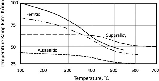
FIGURE 12. Turbine rotor thermal ramp rates for different materials.

Supercritical CO₂ cycle, operating at similar steam conditions as A-USC, is subject to the same considerations and concerns related to the construction materials. On top of that, added complexities associated with this technology are numerous. Operation near the critical point (where fluid properties behave extremely peculiarly), low mass inertia of the turbomachinery, complex turbomachinery configuration and extreme susceptibility to leaks and pressure losses can be counted among them. No field experience is available. Limited amount of dynamic modeling has been done and published. More will be known about the operability of the sCO₂ plant after the test campaign in US DOE’s Supercritical Transformational Electric Power (STEP) facility, a 10 MWe pilot plant, currently in construction at the Southwest Research Institute (SwRI) campus in San Antonio, Texas.

Conclusion

In this study, we looked at steam turbine technology as it stands today and how much further it can be taken. Based on a rigorous cycle analysis drawing upon the second law of thermodynamics, specifically its embodiment in the concept of exergy, it was unequivocally demonstrated that the technology has pretty much reached its zenith. In particular, the second law sets an unambiguous and unassailable theoretical upper limit to cycle efficiency. This upper limit can be readily represented by a simple formula analogous to the Carnot efficiency via mean-effective heat addition and rejection temperatures of the cycle in question. Using this number as a yardstick, the goodness of a given cycle can be determined by how close it can get to it. The proximity of the actual cycle efficiency to the theoretical maximum is quantified by a ratio of the two, which is the technology factor (TF). Modern steam power plant technology is at such a stage of development; TF is in a range of 0.82–85 (world record holder Nordjylland Unit 3 in Denmark is estimated to be around 0.87.)

In terms of a Rankine cycle heat engine, it is unlikely that sCO₂ cycle can be a panacea. It definitely does not fit the bill as a bottoming cycle in a natural gas-fired GTCC (see sCO2 Bottoming Cycle). As a standalone fossil fuel-fired power cycle, at least on paper, it can potentially match the USC or even A-USC and may be slightly better in cycle efficiency but not in net plant thermal efficiency (see sCO₂Standalone Power Cycle). It should be emphasized that sCO₂ Rankine cycle with a fossil fuel-fired “boiler” would require postcombustion carbon capture as well. In addition to increased installed cost, this results in a power plant comprising two blocks with little operational experience and untested (if not truly “first of a kind”) equipment. It is certainly possible that sCO₂ Brayton or Rankine cycle power generation systems can be viable alternatives in unfired applications such as concentrated solar power (CSP), small/modular nuclear and small-scale waste heat recovery²⁸. Even then, small and medium steam turbines for CSP, Cogen, petrochemicals, and small CC applications are going to be hard to beat, especially with advances made in performance optimization (increased steam cycle parameters and design improvements) and operational flexibility by OEMs globally (Pasquariello, 2020).

Data Availability Statement

The original contributions presented in the study are included in the article/Supplementary Material; further inquiries can be directed to the corresponding author.

Author Contributions

The author confirms being the sole contributor of this work and has approved it for publication.

Conflict of Interest

Author SCG was employed by company Bechtel Infrastructure & Power, Inc.

Footnotes

¹It also provides a good look into Russian (i.e., former USSR) steam turbine technology.

²The reason for the moniker “bottoming” will be obvious in Combined Cycle.

³For an ideal gas, this is a true statement. For water/steam, i.e., a “real fluid”, the exact formula is MET = Δh/Δs; MET being equal to the logarithmic mean of temperatures would be conceptually true and numerically close but not exact.

⁴Air Quality Control System.

⁵Thermal Efficiency = Power Output/Fuel Input.

⁶LHV is also known as “net calorific value” and HHV as “gross calorific value.” The difference is the latent heat of condensation of the water vapor, which is a constituent of the combustion products.

⁷Note that (7) is a rough approximation. Gas turbine exhaust energy, as a fraction of GT heat consumption, is slightly lower than (1−η_GT) by about 2% (miscellaneous losses, fuel heating, etc.).

⁸OEMs typically quote steam turbine heat rate, HR_ST = 3,600/η_ST [kJ/kWh], in their heat and mass balances.

⁹Heating, ventilating, and air conditioning.

¹⁰Zero liquid discharge.

¹¹This vital RBC design principle will again come up during the discussion of the suitability of supercritical CO₂ cycle as the bottoming cycle of an advanced GTCC plant (see sCO₂Bottoming Cycle).

¹²Levelized cost of electricity.

¹³3DV™ is a Siemens technology (3-dimensional design with variable reaction levels).

¹⁴There is some disagreement on the steam temperature delineating SC and USC—in some references it is cited as 566°C (1,050°F), in others as 593°C (1,100°F).

¹⁵Balance of plant.

¹⁶https://www.modernpowersystems.com/features/featuretachibana-wan-unit-2-takes-a-supercritical-step-forward-for-japan/, last accessed on September 21, 2020.

¹⁷BoA is the German acronym for lignite-fired power station with optimized plant engineering (“Braunkohlekraftwerk mit optimierter Anlagentechnik”).

¹⁸Of course, if size, material, cost, and/or manufacturing considerations do not allow an optimal LP turbine configuration (number of exhaust ends) with suitably long LSBs, exhaust losses can be significant.

¹⁹This is the reason why rotor blades are referred to as buckets in steam turbine jargon (which sometimes finds its way into gas turbine jargon as well).

²⁰In this context, one must mention the design innovations made by Russian engineers in the USSR, e.g., in LMZ (Leningradsky Metallichesky Zavod), which is the largest Russian manufacturer of power machines and turbines for electric power stations. According to Troyanovskii (2013), “the original design [in LMZ] of the nontraditional meridional contours has nothing like it in world steam turbine engineering”. It is hard to imagine that LMZ designers had 3D CFD at their disposal.

²¹One OEM refers to this design as ISB (Integral Shroud Blade) structure. Continuous coupling of the blades is accomplished by the “untwisting action” of the centrifugal forces during operation. The same OEM has a 1,500/1,800 RPM “half speed” 54 in. titanium blade developed for cross-compound turbines.

²²This corresponds to plant auxiliary load of 12% of the gross. A detailed breakdown of auxiliary power consumption is not available. Nevertheless, it dramatically shows that even with a best-in-class steam turbine, the bottom line, i.e., net power supply to the grid, can get a big hit.

²³The European Cooperation in Science and Technology (COST) is a funding organization for the creation of research networks.

²⁴Reliability, availability, and maintainability.

²⁵Due to its very low cycle PR, i.e., about 3:1, without recuperation, sCO₂ cycle efficiency would be very low because METH and METL would be very close to each other. Graphically, this situation can be readily recognized by the “thinness” of the Brayton and Rankine cycles in Figure 10. Without recuperation, logarithmic means of temperatures in heat addition process (2 → 3) and in heat rejection process (4 → 1) would be quite close to each other. It is easy to see that, in the limit of cycle PR → 1, METH and METL would be exactly equal to each other.

²⁶Note that the split-flow recompression improvement can be applied to the basic recuperated Brayton cycle in exactly the same manner with similar thermal efficiency improvement.

²⁷In 1950s through 1980s, steam turbine startup schemes were devised with thermal stress analysis with the assumption of cylindrical rotor. Stress concentration factors were used to account for deviations from that simplified geometry.

²⁸See Echogen’s EPS100 sCO₂ Rankine cycle waste heat recovery system https://www.echogen.com/our-solution/product-series/eps100/ (last accessed on September 23. 2020).

References

Boss, M. J., Gradoia, M., and Hofer, D. (2005). “Steam turbine technology advancements for high efficiency, high reliability and low cost of electricity,” in Powergen international. Orlando, FL, 14–16

Google Scholar

Bowman, C. F., and Bowman, S. N. (2020). Thermal engineering of nuclear power stations – balance-of-plant systems. Boca Raton, FL: CRC Press

CrossRef Full Text

Cotton, K. C. (1998). Evaluating and improving steam turbine performance. 2nd Edn. Rexford, NY: Cotton Fact Inc.

Cziesla, F., Bewerunge, J., Senzel, A., and Lünen, (2009). “State-of-the art ultra supercritical steam power plant under construction,” in PowerGen Europe 2009 (Germany: Cologne)

Google Scholar

Deckers, M., and Doerwald, D. (1997). Steam turbine flow path optimisations for improved efficiency. Singapore: Powergen Asia

Gülen, S. C. (2013). Performance entitlement of supercritical steam bottoming cycle. J. Eng. Gas Turbines Power 135 (12), 124501. doi:10.1115/1.4007379

CrossRef Full Text | Google Scholar

Gülen, S. C. (2016). Supercritical CO₂—what is it good for? Gas Turbine World, 26–34

Google Scholar

Gülen, S. C. (2017a). “Advanced fossil fuel power systems, chapter 13 in energy conversion,” in Mechanical and aerospace engineering series. 2nd Edn. Editors D. Y. Goswami, and F. Kreith (Boca Raton, FL: CRC Press)

Google Scholar

Gülen, S. C., Yarinovsky, I., and Ugolini, D. (2017b). A cheaper HRSG with advanced gas turbines: when and how can it make sense. Power Eng. 121 (3), 35–42

Google Scholar

Gülen, S. C. (2018). “Combined cycle performance ratings undergo thermodynamic reality check,” in Gas turbine world, 23–32

Google Scholar

Gülen, S. C. (2019a). Gas turbines for electric power generation. Cambridge, UK: Cambridge University Press

Gülen, S. C. (2019b). Gas turbine combined cycle power plants. Boca Raton, FL: CRC Press

Gülen, S. C. (2019c). “Disappearing thermo-economic sanity in gas turbine combined cycle ratings—a critique,” ASME paper GT2019-90883, ASME turbo expo 2019, Phoenix, AZ, June 17–21, 2019. doi:10.1115/gt2019-90883

CrossRef Full Text | Google Scholar

Gülen, S. C., and Smith, R. W. (2010). Second law efficiency of the rankine bottoming cycle of a combined cycle power plant. J. Eng. Gas Turbines Power 132, 011801. doi:10.1115/1.3124787

CrossRef Full Text | Google Scholar

Henderson, C. (2014). Increasing the flexibility of coal-fired power plants, CCC/242. Beijing, China: IEA Clean Coal Centre

Hoffstadt, U. (2001). Boxberg achieves world record for efficiency. Mod. Power Syst. 21 (10), 21–23

Google Scholar

IRENA (2019). Innovation landscape brief: flexibility in conventional power plants. Abu Dhabi: International Renewable Energy Agency

Jansen, M., and Ulm, W. (1995). Modern blade design for improving steam turbine efficiency. VDI-Berichte Nr 1185, 277–290

Google Scholar

Kern, T.-U., Mayer, K. H., Donth, B., Zeiler, G., and DiGianfrancesco, A., (2010). The European efforts in development of new high temperature rotor materials—COST536,” 9th liege conference: materials for advanced power engineering 2010, Liège, Belgium, September 27–29, 2010, 27–36

Google Scholar

Kjaer, S., and Bugge, J. (2004). Europeans still aiming for 700°C steam. Mod. Power Syst. 24 (11), 19–25

Google Scholar

Kotas, T. J. (2012). The exergy method of thermal plant analysis. London, UK: Exergon Publishing Co.

Leyzerovich, A. S. (2008). Steam turbines for modern fossil fuel power plants. Lilburn, GA: the Fairmont Press, Inc.

Meier, H-J., Alf, M., Fischedick, M., and Hillebrand, B. (2004). Reference power plant north rhine-westphalia (PPP NRW). Germany: VGB PowerTech, Vol. 5, 76–89

Moran, M. J., and Shapiro, H. N. (1998). Fundamentals of engineering thermodynamics. New York, NY: John Wiley & Sons, Inc.

Nicol, K. (2015). Application and development prospects of double-reheat coal-fired power units. London, UK: IEA Clean Coal Centre

Oeynhausen, H., Drosdziok, A., and Deckers, M. (1997). Advanced steam turbines for modern power plants. IMechE Paper No. C522/032

Google Scholar

Pasquariello, R. (2020). Steam is here to stay. Turbomachinery International, September 11, 2020, 24–26

Google Scholar

Saito, E., Nishimoto, S., Endo, H., Yamamoto, R., Kawasaki, K., and Sato, J. (2017). Development of 700°C class steam turbine technology. Mitsubishi Heavy Industries Technical Rev. 54 (3), 10–15

Google Scholar

Simon, V., and Oeynhausen, H. (1998). “3DV™ three-dimensional blades—a new Generation of steam turbine blading, PWR-33,” 1998 International joint power generation conference, Baltimore, MD, August 23–26, 1998, 2, 71–78

Google Scholar

Simon, V., Stephan, I., Bell, R. M., Capelle, U., Deckers, M., Schnaus, J., et al. (1997). “Axial steam turbines with variable reaction blading,” Proceedings of the 4th international charles parsons turbine conference, advances in turbine materials design and manufacturing, 46–60

Google Scholar

Steam (2015). Steam. 42nd Edn. Editor G. L. Tomei (Charlotte, NC: The Babcock & Wilcox Company)

Stodola, A. (1927). Steam and gas turbines. Authorized translation from the sixth German edition by Dr. L. C. Loewenstein. volumes one and two. New York, NY: McGraw-Hill Book Company, Inc.

Troyanovskii, B. M. (2013). The new design of the low-pressure cylinders of mitsubishi steam turbines. Therm. Eng. 50 (2), 170–172

Google Scholar

VGB PowerTech Guideline (1990). Thermal behaviour of steam turbines. Revised 2nd Edn. Essen, Germany: VGB-R105e, VGB PowerTech Service GmbH

Viswanathan, R., Armor, T., and Booras, G. (2004). A critical look at supercritical power plants. Power Magazine, April 2004, 42–49.

Google Scholar

Zachary, J., and Koza, D. (2006). The long and short of last-stage blades. Power Magazine, December 2006

Google Scholar

Zörner, W. (1994). Steam turbines for power plants employing advanced steam conditions. 10th CEPSI, September 1994. Christchurch, New Zealand, 19–23

Google Scholar