A Markov Regime Switching Model for Ultra-Short-Term Wind Power Prediction Based on Toeplitz Inverse Covariance Clustering

Introduction

Wind energy has grown very fast recently, the new installed capacity of global onshore wind power in 2019 has reached 60.4 GW (Lee et al., 2020). With the large-scale integration of wind power, ultra-short-term wind power prediction plays a significant role. It is not only crucial for the stable operation of the power system but can provide useful information for the intraday and real-time electricity market. Therefore it is urgent to develop a prediction system with high accuracy, especially for the regional wind farms.

There has been a lot of methods for ultra-short-term wind power prediction. Those methods can be roughly divided into two classes, namely the physical model method (Feng et al., 2010) and the statistical learning method (Xue, et al., 2015). The physical method is based on the detailed modeling of the atmosphere movement. It can simulate the nonlinear characteristics of the wind power time series but is time-consuming and its performance is highly dependent on the accuracy and complexity of the model (Peng, et al., 2016). The statistical learning methods include the multivariate vector autoregressive (VAR) method (Zhao, et al., 2018), Gaussian process regression method (Kou, et al., 2013), machine learning method (Demolli, et al., 2019), deep learning method (Khodayar and Wang, 2018; Lai, et al., 2018) and hybrid method (Duong, et al., 2013; Wang, et al., 2019). But most of them are based on one state prediction, which means it uses one single model for all the scenarios. However, the spatiotemporal relationship of the wind farms is time variant due to the change of the atmospheric condition, there are different kinds of spatiotemporal pattern (Xiong et al., 2016). Therefore, it can be more reasonable to use a different prediction model for different time which shares a similar spatiotemporal pattern. In this way, the deep learning method can be utilized more effectively. Hamilton (1989) brought out the concept of regime switching in the time series prediction. The effectiveness of the Markov regime switching has been witnessed in many areas. Song et al., (2014) uses the Markov switching model to predict wind power. Research (Hu et al., 2014) has brought out a G eneralized Principal Component Analysis (GPCA) method to divide time series into several parts and predict the wind speed using different models. Xiong et al., (2019) adopts K-means for the clustering of NWP and uses Support Vector Regression (SVR) for the prediction of wind power in each cluster. There are even some online learning methods such as Least Absolute Shrinkage and Selection Operator (LASSO) (Messner and Pinson, 2019) and Extreme Learning Machine (Park and Kim, 2017) which can adjust the parameter in real-time to adapt to the pattern changes of the wind system. Sun et al., (2020) also developed a reinforcement learning method to choose the wind power prediction model dynamically to adopt to the time-variant wind process.

The wind power sequence hidden regime discovery is closely related to the time series subsection. Lavielle and Lebarbier (2001) brings out a change-point detection model to segment the time series based on MCMC. However, when dividing the time series, the spatiotemporal correlation is not considered and the optimal dividing number is also not discussed. The Probabilistic Graph Model (PGM) is a classical method to describe the correlation among variables and has been used to describe the spatiotemporal relationship of energy time series (Wytock and Kolter, 2013). Based on that, Hallac et al., (2017) has provided a subsequence clustering method for multivariate time series called Toeplitz Inverse Covariance-based Clustering (TICC) to discover the hidden regimes in temporal data. It can characterize the interdependencies between different observations in a typical subsequence of that cluster by defining a correlation network of multivariate time series. The proposed TICC method has been tested in an automobile dataset to discover the different driving behavior such as slowing down, turning, and speeding up. Liu et al., (2020) also used the sparse inverse covariance matrix to divide the wind direction pattern for the wind speed prediction. But there are a lot of hyper-parameters which are needed to be determined in the method such as the regime number. Besides when the observation variable is large, the performance of the TICC method is not stable due to the inverse calculation of the covariance matrix. In the traditional TICC method, the BIC criterion is used to determine the best value cluster number. However, this kind of method is more closely related to the model complexity rather than the distribution of the data. In some research (Jiang et al., 2013), Bayesian posterior probability is used to determine the regime number of the Markov switching model. In some cases, KL divergence is used to select the best model (Smith et al., 2006).

Inspired by those researches, we design an ultra-short-term wind power prediction framework that consists of four sub-modules. In the first module, we design a graph autoencoder that can reduce the dimension of historical wind power, NWP data, and future wind power into a lower dimension which is suitable for the TICC method. In the second module, the state of the wind farm cluster is determined by the dimension reduction result and the regime division result is worked out according to the TICC method. KL divergence between the original distribution and the distribution after the division is calculated to determine the optimal regime number. The third module is making use of the dimension reduction results to predict the next regime and the fourth module is using the corresponding model of the regime for the wind power prediction.

The main contributions of this paper are summarized as follows.

(1) We propose a dimension reduction method for the state representation based on the graph autoencoder which is easy to be implemented and can preserve the spatiotemporal relationship of the wind farms in the reduced dimension.

(2) We adopt the TICC method for the time series segmentation which can consider the spatiotemporal relationship to find the most meaningful subsection of time series compared to other clustering methods.

(3) We also employ the KL divergence criterion to determine the optimal value of cluster number $N_p$. The spatiotemporal graph convolutional network for wind power prediction is used for each segmentation and the prediction results are verified on wind farms located in Northeast China. It can reduce normalized root mean square error (RMSE) in the fourth hour by nearly 0.5% compared to other Markov regime switching models.

The rest of this paper is organized as follows. Ultra-Short-Term Wind Power Prediction Framework introduces the ultra-short-term wind power prediction framework. Toeplitz Inverse Covariance Matrix for Time Series Clustering presents the algorithms to solve Toeplitz Inverse Covariance-based Clustering for the wind farm time series clustering and uses graph autoencoder network for the dimension reduction of wind farm states. Optimal Regime Number Calculation Based on MCMC describes the MCMC method to generate time series under different regime numbers and uses the KL divergence to determine the optimal clustering number. The Regime Transition Prediction in Markov Switching Method describes the Markov switching mechanism of the prediction method. Case Study conducts a comprehensive case study to verify the effectiveness of this method.

Ultra-Short-Term Wind Power Prediction Framework

The Markov Regime Switching Model

Wind farm cluster power prediction is a multi-variable time series prediction problem. The most likely output in the next $H$ time steps should be predicted according to the wind power observation in the previous $M$ time steps and NWP data of length $N$. The prediction method is the modeling of the chaotic wind system and can be described as follows.

$y_t=f\left(x_t\right),(1)$

$y_t=\left[P_{t+1},\dots ,P_{t+H}\right],(2)$

$x_t=\left[P_{t-M+1},\dots ,P_t,V_{t+1},\dots ,V_{t+N}\right],(3)$

where $P_{t-M+1},\dots ,P_t$, $V_{t+1},\dots ,V_{t+N}$, and $P_{t+1},\dots ,P_{t+H}$ are the historical wind power, NWP windspeed and predicted wind power respectively. $x_t$ is the input of the prediction model and $y_t$ is the output of the model. However, for such a complex chaotic system, using one function to model may cause more error. Therefore, the Markov regime switching model is brought out as follows.

$y_t={\displaystyle {\sum }_{i=1}^K{\mu }_i{f}_i\left(x_t\right)},(4)$

${\mu }_i=\{\begin{array}{c}0,x_t\in {\theta }_i \\ 1,x_t\notin {\theta }_i\end{array}.(5)$

In the Markov regime switching model, the class of the input variable $x_t$ is judged and the parameter ${\mu }_i=1$ only when $x_t$ belongs to the corresponding class ${\theta }_i$. $K$ is the number of regimes in the Markov switching model. In fact, it is the piecewise approximation of the complex chaotic system.

Wind Farm Cluster Ultra-Short-Term Wind Power Prediction Framework

We present a comprehensive ultra-short-term wind power prediction framework which consists of four modules. The framework is shown in Figure 1.

FIGURE 1

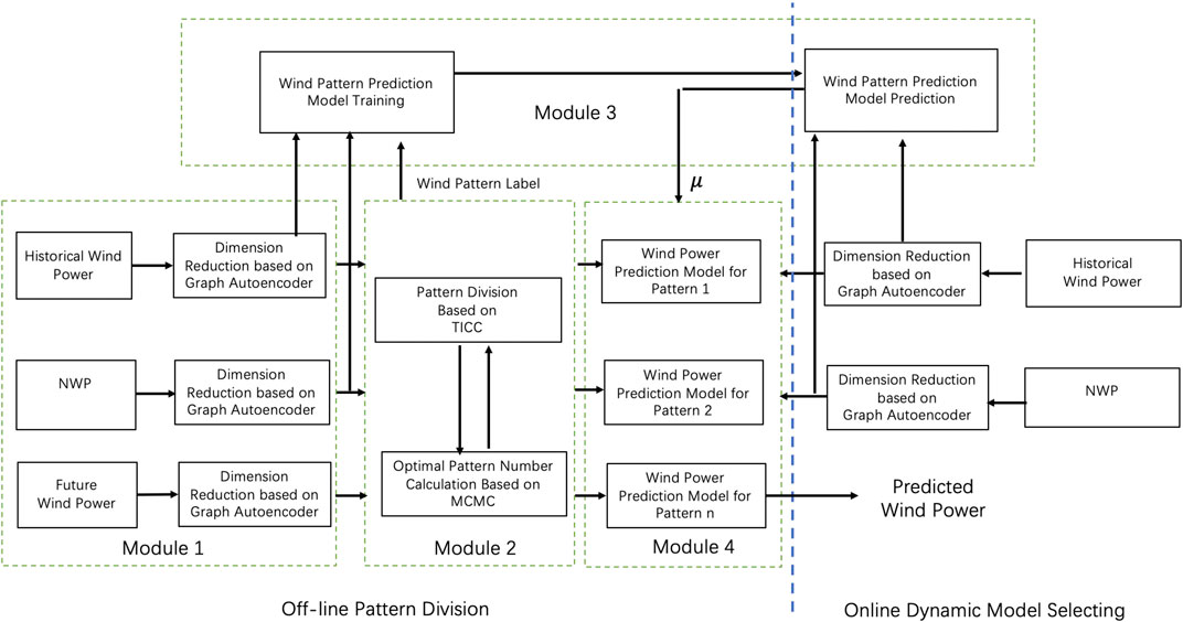
FIGURE 1. The framework of ultra-short-term wind power prediction.

First, we develop a state dimension reduction method for the future wind power, historical wind power and NWP information based on the graph autoencoder neural network. Second, according to the state embedding result, we use a probabilistic graph model based method to cluster the operation state of the wind farms which can consider the spatiotemporal relationship among wind farms. We also use the KL divergence and MCMC to determine the number of regimes. Third, for each regime, we use a spatiotemporal graph model to predict the wind power and each model has different weights. Fourth, by utilizing the state dimension reduction and regime division result, we can predict the next state and select the corresponding prediction model.

Toeplitz Inverse Covariance Matrix for Time Series Clustering

Problem Formulation and Description

When predicting the wind power, the observation of a wind farm is not only correlated with observations before, but also correlated with observations of adjacent wind farms. So, we can have a formulation as follows. For a time series of T sequential observations,

$X_{orig}=\left[x_1,x_2,x_3,\dots ,x_T\right],(6)$

where $x_1$ is the first multivariate observation. In order to classify this measurement into $K$ groups, we not only consider the current observation $x_t\in R^n$, but also the historical observation of time window whose length is $w$. This time series segment $X_i\in R^{nw}$ contains measurements $x_{t-w+1},x_{t-w+2},\dots ,x_t$. In this way, adjacent time series fragments can belong to the same class as much as possible.

In the TICC method, a block Toeplitz matrix to represent the cluster $i$ is constructed. Each ${\text{Θ}}_i$ is a $nw\times nw$ matrix and can be described as follows (Hallac et al., 2017).

${\text{Θ}}_i=\left[\begin{array}{lllll}{A}^{\left(0\right)}\hfill & {\left(A^{\left(1\right)}\right)}^T\hfill & {\left(A^{\left(2\right)}\right)}^T\hfill & \cdots \hfill & {\left(A^{\left(1\right)}\right)}^T\hfill \\ A^{\left(1\right)}\hfill & A^{\left(0\right)}\hfill & {\left(A^{\left(1\right)}\right)}^T\hfill & \ddots \hfill & ⋮\hfill \\ A^{\left(2\right)}\hfill & A^{\left(1\right)}\hfill & \ddots \hfill & \ddots \hfill & ⋮\hfill \\ ⋮\hfill & \ddots \hfill & \ddots \hfill & {\left(A^{\left(1\right)}\right)}^T\hfill & {\left(A^{\left(2\right)}\right)}^T\hfill \\ ⋮\hfill & \ddots \hfill & \ddots \hfill & A^{\left(0\right)}\hfill & {\left(A^{\left(1\right)}\right)}^T\hfill \\ A^{\left(w-1\right)}\hfill & \cdots \hfill & \cdots \hfill & A^{\left(1\right)}\hfill & A^{\left(0\right)}\hfill \end{array}\right],(7)$

where, $A^{\left(0\right)}$, $A^{\left(1\right)}$, …, $A^{\left(w-1\right)}\in R^{n\times n}$ and for each sub-block $A^{\left(0\right)}$ represents the temporal correlation. So $A_{ij}^{\left(0\right)}$ represents the correlation between wind farm $i$ and wind farm $j$ at time $t$. For the MRF of each cluster, $A^{\left(0\right)}$ represents the correlation matrix between the vertexes in each layer. For example, $A_{ij}^{\left(1\right)}$ represents the correlation of wind farm $i$ at time $t$ and wind farm $j$ at time $t-1$. $A_{ij}^{\left(2\right)}$ represents the correlation of wind farm $i$ at time $t$ and wind farm $j$ at time $t-2$ The block Toeplitz structure of the inverse covariance matrix means that we make a time-invariant assumption within the time length of $w$ (generally, the length of the time window $w$ is required to be much shorter than sequence length $L$), so that the connection between each layer will exist. We make this assumption because we are looking for a unique structural regime to divide each group. We think that each group belongs to a specific regime and they also maintain a same specific structure in the whole time series.

In the TICC method, each subsection is assumed to be subject to multivariate gaussian distribution and can be represented by Markov Random Field (MRF) ${\text{Θ}}_i$. According to the probabilistic graphical model, when the subsection is subjected to multivariate Gaussian distribution, it can be represented by a gaussian inverse covariance matrix ${\text{Θ}}_i\in R^{nw\times nw}$. ${\text{Θ}}_i$ is a crucial parameter in the TICC model because it not only represents a kind of wind pattern, but is also a regime in the Markov switching model. It can provide a more interpretable representation for the cluster results and the sparsity of inverse covariances is also a kind of way to prevent over-fitting. According to the definition, our goal is to solve the $K$ gaussian inverse covariance matrix $\text{Θ}={\text{Θ}}_1,{\text{Θ}}_2,\dots ,{\text{Θ}}_K$ by allocating the $T$ observations into $K$ cluster. The specific process can be realized by solving the optimization problem as follows (Hallac et al., 2017).

$\underset{\text{Θ}\in \text{Γ},P}{\text{argmin}}{\displaystyle {\sum }_{i=1}^K\left[\Vert \lambda \circ {{\text{Θ}}_i}_1\Vert +{\displaystyle {\sum }_{X_i\in P_i}\left(-ll\left(X_t,{\text{Θ}}_i\right)+\beta X_{t-1}\notin {\theta }_i\right)}\right]}.(8)$

This problem is called Toeplitz inverse covariance-based clustering (TICC) problem (Hallac et al., 2017). Where, $\text{Γ}$ is the set of symmetric Toeplitz matrix ${\text{Θ}}_i$. $\lambda \circ {{\text{Θ}}_i}_1$ is the $l_1$ norm of Hadamard product between $\lambda$ and sparse inverse covariance matrix. Besides, $ll\left(X_t,{\text{Θ}}_i\right)$ is the log-likelihood. $X_t$ is the sample from cluster $i$. In formulation Eq. 8, $\beta$ is a parameters of time continuity, $X_{t-1}\notin {\theta }_i$ is a function of time continuity. The computation method of $ll\left(X_t,{\text{Θ}}_i\right)$ is in Eq. 9.

$ll\left(X_t,{\text{Θ}}_i\right)=-\frac{1}{2}{\left(X_t-{\mu }_i\right)}^T{\text{Θ}}_i\left(X_t-{\mu }_i\right)+\log \det {\text{Θ}}_{i^{\mathbf{-}}}\frac{n}{2}\log \left(2\pi \right),(9)$

where ${\mu }_i$ is the empirical mean of cluster $i$. There are two regularized parameters in the TICC optimization problem: $\text{λ}$ which are used to represent the sparsity of each group’s Markov random field and $\text{β}$, the penalty function of smoothness to motivate the adjacent time series segments to come from the same class. Even $\text{λ}$ is a matrix of $nw\times nw$ dimension, we fix all the values on a single constant and reduce the search space to one parameter. In practical application, the value of $\text{λ}$ is 11e-3 and $\beta$ is 350.

The objective function Eq. 8 in the TICC method is a hybrid combination and continuous optimization problem. There are two groups of variables, namely, the clustering group $P$ and the inverse covariance matrix $\text{Θ}$. The coupling of the two variables makes the problem highly nonconvex. Therefore, there is no feasible way to find the global optimal solution. TICC algorithm divides the clustering of time series segments into two subproblems. The first one is to allocate each point to a different group by using a dynamic programming method. The second one is to learn the parameters of Markov random fields in each group by using a graphic lasso method. Then the alternating direction method of multipliers (ADMM) is used to solve the graphic lasso (Boyd et al., 2011). Finally, the expectation maximization (EM) algorithm is used to solve the two above problems alternatively. The details of the algorithms can refer to the work by Hallac et al., (2017).

But it should be noted that $X_t$ is a continuous fragment $x_{t-w+1},x_{t-w+2},\dots ,x_t$ and is a vector of dimension $nw$. Toeplitz matrix assumes that every cluster has a time-invariant structure and the length of time window w is usually not set to be very large. Because larger time window $w$ will make the parameters of Toeplitz matrix grows at the rate of square and disobey the time-invariant assumption. Besides, according to the definition of $x_t$ in Eq. 3, the temporal relationship is already considered. Empirically, $w$ is set as three in the following test. But another parameter, the cluster number $K$ is very important, because it determines there are how many regimes. The method to determine the best value of cluster number $K$ will be discussed in Optimal Regime Number Calculation Based on MCMC.

Operation State Representation of Wind Farm Cluster

Wind farm cluster usually contains 10–20 wind farms and the variables that can be obtained include historical wind power and NWP information. Therefore, according to Eq. 3, $x_t\in R^n$ is a high dimension vector. For example, suppose the current time is $t$, training data which is very important for the ultra-short time wind power prediction includes historical wind power data $P_{t_0-40}$, $P_{t_0-39}$, …, $P_{t_0}$ and future NWP wind speed data $V_{t_0}$, $V_{t_0+1}$, …, $V_{t_{0+20}}$. The NWP wind speed usually contains wind speed from four different altitudes. For 20 wind farms in a region, the dimension of measurement data at $t$ can reach 2,400. In the TICC method, the dimension of Toeplitz matrix is $2400\cdot w$, it is obviously unacceptable and unnecessary in the correlation analysis. Therefore, it is significant to use the dimension reduction method for the computation.

There are a lot of dimension reduction methods such as principal component analysis (PCA) and nonlinear manifold learning methods. However, PCA is a kind of linear process and cannot reflect the nonlinear characteristic of the data. Even manifold learning can learn about the nonlinear feature of the data, it is time-consuming especially when the data set is large. It is not suitable for online application. Besides, we also want to preserve the spatiotemporal relationship in the dimension reduction process. Autoencoder is a kind of neural network which is convenient for dimension reduction and online application. The feature and information in the original data can be preserved in the dimension reduction results according to the different designs of neural networks in the autoencoder (Goodfellow et al., 2016). Therefore, we can use the graph autoencoder method for dimension reduction and the process is represented as follows.

$S_P=h_p\left(P_{t-M+1},\dots ,P_t\right),(10)$

$S_V=h_V\left(V_{t+1},\dots ,V_{t+N}\right),(11)$

$S_f=h_f\left(P_{t+1},\dots ,P_{t+H}\right),(12)$

where $h_p$, $h_V$, and $h_f$ are the graph autoencoder for the historical wind power, NWP windspeed and future wind power respectively. $S_P$, $S_V$, and $S_f$ are the dimension reduction results. The autoencoder can also reconstruct the original data from the dimension reduction results.

${\widehat{P}}_{t-M+1},\dots , {\widehat{P}}_t=h_p^{-1}\left(S_P\right),(13)$

${\widehat{V}}_{t+1},\dots , {\widehat{V}}_{t+N}=h_V^{-1}\left(S_V\right),(14)$

${\widehat{P}}_{t+1},\dots , {\widehat{P}}_{t+H}=h_f^{-1}\left(S_f\right),(15)$

where ${\widehat{P}}_{t-M+1},\dots , {\widehat{P}}_t$, ${\widehat{V}}_{t+1},\dots , {\widehat{V}}_{t+N}$, and ${\widehat{P}}_{t+1},\dots , {\widehat{P}}_{t+H}$ are the reconstructed historical wind power, NWP information and future wind power respectively. The loss function of the graph autoencoder is the difference between the original data and the reconstructed data which is called the reconstructed error.

$J\left(W,b\right)=\sqrt{\frac{1}{m}{\displaystyle {\sum }_{i=1}^m{\left(\widehat{x}-x\right)}^2}},(16)$

where the $x$ is the input the graph autoencoder and $\widehat{x}$ is the reconstructed data. In this case, $x$ can be historical wind power $P_{t-M+1},\dots ,P_t$, NWP information $V_{t+1},\dots ,V_{t+N}$ and future wind power $P_{t+1},\dots ,P_{t+H}$. The training process of the graph autoencoder is minimizing the reconstructed error. The architechture of the graph autoencoder is in Figure 2.

FIGURE 2

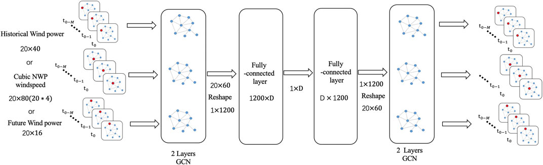
FIGURE 2. The architecture of graph autoencoder.

In this case, we designed three graph autoencoders with the same architecture for historical wind power, NWP windspeed and future wind power respectively. But the reduced dimension $D$ is a very important value in graph autoencoder. It should be noted that, the wind power is proportional to the cubic wind speed (Duong, et al., 2014; Duong, et al., 2015). According to previous research (Fan, et al., 2020), the cubic wind speed can represent the tendency of the wind power more precisely. Therefore, the cubic NWP windspeed is used as the input in this model rather than NWP windspeed. We can get its value according to the reconstructed error of the graph autoencoder. When the reconstructed error is reduced into a satisfying value or the increase in the reduced dimension can hardly decrease the reconstructed error, the reduced dimension can be determined. The dimension reduction results are used as the input of TICC to replace the original measurement data which can make the regime division easier to be implemented.

Optimal Regime Number Calculation Based on MCMC

Kullback-Leibler Divergence Criterion

KL divergence is also called relative entropy. If there are two separate distributions $P\left(x\right)$ and $Q\left(x\right)$ for the same random variable $x$, we can use KL divergence to measure the difference between the two distributions. In machine learning, $P$ is often used to represent the real distribution of samples and $Q$ is used to represent the distribution generated by the model. Then KL divergence can be used to calculate the difference between the two distributions, that is, the loss value.

$D_{KL}\left(p\Vert q\right)={\displaystyle {\sum }_{i=1}^n\left(x_i\right)\log \left(\frac{p\left(x_i\right)}{q\left(x_i\right)}\right)}.(17)$

It can be seen from the formula that the more similar the distribution of $P$ is to that of $Q$, the smaller the divergence value is. But in a general calculation, the divergence value of the arbitrary distribution is difficult to calculate, so Gaussian distribution is often used for the approximate solution. The KL divergence of two high dimensional Gaussian distributions can be calculated by the following formula (Murphy, 2012).

$D_{KL}\left(p\Vert q\right)=\frac{1}{2}\log \frac{\left|{\Sigma }_2\right|}{\left|{\Sigma }_1\right|}-n+tr\left({\Sigma }_2^{-1}{\Sigma }_1\right)+{\left(u_2-u_1\right)}^T{\Sigma }_2^{-1}\left(u_2-u_1\right),(18)$

where ${\Sigma }_1$ and ${\Sigma }_2$ are the covariance matrix of $P$ and $Q$. Therefore, when measuring the distribution difference between two datasets, we can first use high-dimensional Gaussian distribution to fit and then use the above formula to calculate the distance.

Model Selection Based on Markov Chain Monte Carlo Simulation

In the TICC method, each regime is an $n$ dimension Gaussian distribution and the covariance of each regime is given. First, we solve the different mean values and variance of each regime. The transition probability of each regime can also be worked out. Then, the MCMC sampling method is used to generate a new $n$ dimension time series. For each step in the MCMC sampling, we determine the regime according to the transition probability and sample the specific value of wind power according to the parameter of the fitted $n$ dimension Gaussian distribution. Next, the mean value and variance of the new Gaussian distribution according to the generated time series can be solved, and the KL divergence is used to calculate the difference between the original data and the generated data. The schematic diagram is in Figure 3.

FIGURE 3

FIGURE 3. Kl distance calculation based on MCMC.

We can choose different regime numbers for the TICC clustering and use the MCMC to generate data set. Then the KL distance of the original data set and the generated data set is calculated. According to the curve between KL distance vs. the regime number and some domain knowledge such as the size of the training data and the maneuverability in engineering, we can determine the optimal regime number.

The Regime Transition Prediction in Markov Switching Method

The State Transition of Wind Power Prediction

According to Eqs 4, the corresponding model is chosen for the specific regime. But there is a concern that we don’t know what the regime is in the prediction process. Therefore, we need to design a prediction model to choose the corresponding model according to the dimension reduction results of historical wind power and NWP information. The prediction process is in Figure 4.

FIGURE 4

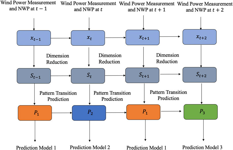
FIGURE 4. The regime transition of wind power prediction.

We can see from the figure that there are two prediction models in the Markov switching model actually. The main model is used to predict the wind power in the next 4 h and the auxiliary model can predict the regime in the next 4 h and choose the approximate main prediction model.

The Prediction Models for the Regime Transition and Wind Power

In this case, we use the ELM as the auxiliary model for the regime transition prediction. ELM is a kind of fast learning algorithm which is suitable for the real-time regime estimation (Huang et al., 2006). For the single hidden layer neural network, ELM can initialize the input weight and bias randomly and get the corresponding output weight. For a single hidden layer neural network, there are $M$ arbitrary samples $S$ and their labels $v$, where $S\in R^{M\times 2D}$, $v\in R^{M\times 1}$. For a single hidden layer neural network with $L$ hidden layer node, it can be represented as

${\displaystyle \sum _{\mathbf{i}=1}^{\mathbf{L}}{\mathbf{\beta }}_{\mathbf{i}}\mathbf{\sigma }\left({\mathbf{W}}_{\mathbf{i}}\cdot {\mathbf{S}}_{\mathbf{j}}+{\mathbf{b}}_{\mathbf{i}}\right)={\mathbf{v}}_{\mathbf{i}}},\mathbf{j}=1,\dots ,\mathbf{M}.(19)$

where ${\mathbf{\beta }}_{\mathbf{i}}$, ${\mathbf{W}}_{\mathbf{i}}$, and ${\mathbf{b}}_{\mathbf{i}}$ are the parameter of the ELM. $\mathbf{\sigma }$ is the kernel activation function and we use Gaussian kernel here. The input of the ELM is the dimension reduction results of the historical wind power and NWP information. The output is the label of the regime which is used to select the corresponding spatiotemporal graph convolutional wind power prediction model. The objective of the auxiliary model is maximizing the prediction accuracy of the regime class. In this case, ${\mathbf{v}}_{\mathbf{i}}$ is the regime class and is a integer from 1 to $K$. In practice, ${\mathbf{v}}_{\mathbf{i}}$ should be transformed into a $K$ dimension one hot encoding vector $\mu$ in the Markov switching model (Pedregosa, et al., 2011).

For the main prediction model, a spatiotemporal graph convolutional network named M2GSNet is used for the wind power prediction (Fan, et al., 2020). The performance of M2GSNet has been verified in the practical engineering, so we use it as the main model for wind power prediction here. The input of the M2GSNet is the historical wind power and cubic NWP windspeed. The output is the predicted wind power of each wind farm and the sum of the wind power is the wind power of the wind farm cluster.

Case Study

Data Description and Test Environment

The data of wind farm clusters located in Northeast China are used for the case study. The whole capacity of the wind farm cluster is 2854.31M and the location of those wind farms is in Figure 5. The wind power and NWP data are used for the analysis. NWP data include wind speed from four different altitudes (170 m wind speed, 100 m wind speed, 30 m wind speed, 10 m wind speed). The training set containing 13,000 samples (from 2019-01-01 08:15:00 A.M. to 2019-05-16 06:00:00 P.M.), validate set containing 2,000 samples (from 2019-01-01 08:15:00 A.M. to 2019-05-16 06:00:00 P.M.) and testing set containing 1,000 samples (from 2019-01-01 08:15:00 A.M. to 2019-05-16 06:00:00 P.M.). The sampling interval is 15 min. The proposed method is tested on Linux server Cluster (CPU: Intel Xeon (R) CPU E5-2650 v4 @ 2.10 GHz, GPU: NVIDIA Tesla P100) and deep learning framework Pytorch (1.4.0).

FIGURE 5

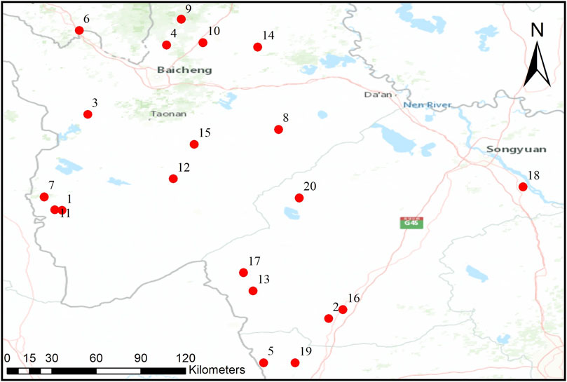
FIGURE 5. The location of the wind farms.

The output of ultra-short-term wind power prediction is the wind power of this region which is the sum of every wind farm. The adjacent matrix which will be used in the autoencoder and spatiotemporal graph convolutional wind power prediction network is very important for the spatial-temporal dependency modeling. The wind farms are located in a region and the spatial dispersion is mostly reflected by the distance among wind farms. Therefore, we use the Gaussian kernel threshold distance function to define the adjacent matrix.

$A_{i,j}=\{\begin{array}{l}{e}^{\frac{\text{dist}{\left(i,j\right)}^2}{{\text{std}}^2}},\text{if}\text{dist}\left(i,j\right)\le \epsilon \hfill \\ 0,\text{otherwise}\hfill \end{array},(20)$

where $\text{dist}\left(i,j\right)$ is the geographical distance between wind farm $i$ and wind farm $j$. $\text{std}$ is the standard deviation of the distance among $n$ wind farms. $\epsilon$ is the threshold and we use half of the mean distance as the threshold. Here we set the value of $\epsilon$ as 0.6. When the distance of wind farm $i$ and wind farm $j$ is smaller than the $\epsilon$, we assess there is no connection between them. The wind power and cubic wind speed have different units, so normalization is used to reduce the effect of different units.

$x=\frac{x_m-x_{\min }}{x_{\max }-x_{\min }}.(21)$

The root mean square error (RMSE) and mean absolute error (MAE) is selected to assess the performance of the model on the testing set.

$\mathrm{RMSE}=\sqrt{\frac{1}{n_s}{\displaystyle {\sum }_{i=1}^{n_s}{\left(x_{ti}-{\widehat{x}}_{ti}\right)}^2}},(22)$

$\mathrm{MAE}=\frac{1}{n_s}{\displaystyle {\sum }_{i=1}^{n_s}\left|x_{ti}-{\widehat{x}}_{ti}\right|},(23)$

where $x_{ti}$, ${\widehat{x}}_{ti}$ are the normalized true value and normalized predicted value in prediction scenario $i$ at prediction time step $t$. $n_s$ is the number of samples in the test set. The wind power of the past 10 h and the cubic NWP windspeed of the next 5 h are used for wind power prediction (Fan, et al., 2020). The structure in Figure 2 is also used for the dimension reduction of historical wind power, cubic NWP windspeed and future wind power. Since the time range of ultra-short-term wind power prediction is the next 4 h, the length of historical wind power is 40 time steps in this dimension reduction model. The NWP sample including 20 time steps and the future wind power includes 16 time steps.

Since it is impossible to do the grid search on the whole parameter space, the hyper-parameters are determined according to the grid search combined with human experience. The hyper-parameters of the spatiotemporal model used for wind power prediction are the same in the reference paper (Fan, et al., 2020). Therefore, the iteration epoch of model for wind power prediction is 200 and the training batch size is 256. The optimizer is Adadelta and the learning rate is 0.1. The five-fold cross-validation is used for verification. In the dimension reduction model, the learning rate for dimension reduction model is chosen from the set (0.01, 0.05, 0.1, 0.15, 0.2, 0.25, 0.3, 0.35, and 0.4) and the hidden state for the graph convolutional network is chosen from the set (10, 20, 30, 40, 50, 60, 70, 80, 90, and 100). The reconstruction error of the graph autoencoder are used to determine the optimal value. Finally, the optimizer in the graph autoencoder is Adadelta and the learning rate is 0.05. The hidden state in the graph autoencoder is 60. The hyper parameter of the TICC state division method is $\lambda$ and $\beta$. By refer to related research (Hallac et al., 2017), they were chosen by hand. The principal is to make the TICC method more likely to be convergent. Finally, the $\lambda$ is 11e-3 and $\beta$ is 350. In the auxiliary model ELM for regime transition prediction, the main hyper-parameter is the hidden state. It is selected from the set (10, 20, 30, 40, 50, 60, 70, and 80). The selection rule is maximizing the regime prediction accuracy and the value in the final model is 30.

Dimension Reduction of Wind Farm Cluster State

Before using the TICC method for the state division, we should reduce the dimension of the wind farm cluster. We use the graph autoencoder to reduce the dimension of historical wind power, NWP and future wind power separately. After that, we concatenate the dimension reduction results as the input of the TICC method. To determine the reduced dimension, the reconstruction error is computed to determine the appropriate dimension in Figure 6.

FIGURE 6

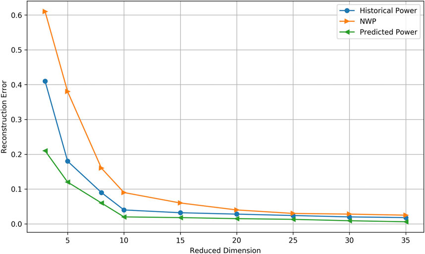
FIGURE 6. The construction error of different dimension.

From this figure, when the dimension is reduced to 10, the reconstruction error can decrease to an acceptable level. Therefore, we concatenate three 10 dimension vector to represent the state of the wind farm cluster.

Regime Discovery Based on TICC

Through the observation of dimension reduction results, it can be found that the operation state of the wind farm is indeed divided into several segments in a period of time, so it is reasonable to use the clustering method to deal with them separately. The KL value of different regime numbers by TICC is as follows.

We can see from Table 1 that with the increase of the regime number, the KL divergence is reducing. It is understandable since the more the state number, the more meticulous that the model can describe the statistical distribution feature of the data and the KL divergence is smaller. But the regime number shouldn’t be too large because it will make the prediction model too complex. So it is significant to choose the appropriate regime number. We choose the first local minimum of the KL divergence and regime number curve as the regime number. In this case, we divide the time series of the wind farms into three regimes. Because if too many regimes are divided, there are only a few samples in some regimes. It is not adequate to train the prediction model which may lead to the underfitting of the model. According to the divided results, each regime can use the prediction model of the current regime separately. We also visualize the divided regime of the validate set when the regime number is 3 and 4. The sum wind power of the wind farms divided by different regimes is also marked by a different color. The results are as follows.

TABLE 1

TABLE 1. The KL value of different regime number (10^6).

From Figure 7, we can see that when the wind power time series of the wind farm cluster are divided into three regimes, the states of the wind farms are reasonably represented. But when the time series is divided into more regimes, there are only a few samples in some types which is not convenient for the model training. We also visualized the sparse inverse covariance matrix which stands for different regimes to illustrate this.

FIGURE 7

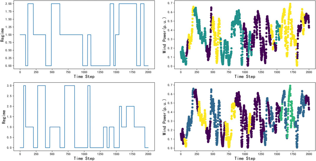
FIGURE 7. The wind power time series regime division.

In the heatmaps, the sparse inverse covariance matrix is a 90 * 90 matrix because the dimension of the concatenated dimension reduction vector is 30 and $w$ is set to three according to the description in 3.1. The first array of Figure 8 is the heatmaps of the full sparse inverse covariance matrix and the second array is a 30 * 30 submatrix from the upper left corner of the inverse covariance matrix which is also represented as $A^{\left(0\right)}$. We can notice that there is a distinct difference among the three regimes.

FIGURE 8

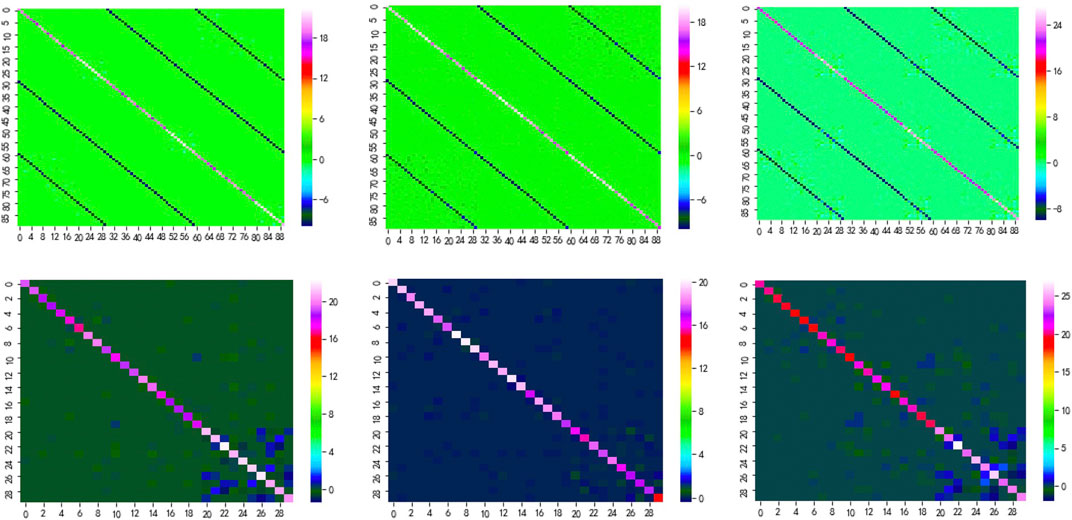
FIGURE 8. The patterns of sparse inverse covariance matrix estimated by TICC

The Prediction Results of TICC Method

Graph convolutional network is a kind of method which can take consideration of the spatial-temporal relationship of the wind farms. Based on this idea, the historical wind power data and future numerical weather forecast wind speed data of wind farms are used to predict the power of wind farm cluster for next 4 h. The results of a single state model and the Markov switching prediction method are compared, as shown in the figure below.

In Figure 9, the RMSE of a single model, TICC method when the regime is known and TICC method when the regime is unknown in the fourth hour is 8.10, 7.24, and 6.95% respectively. We can see that the prediction results of the multi-model are better than the prediction results of the single prediction model. We also compare the prediction results of known category and unknown category since in the realistic situation, the state of the wind farm is unknown and we should use the ELM algorithm for the prediction which will lead to some errors. The accuracy of the ELM to predict the regime is 87.63%. But the results in Figure 9 show that even there are some errors in the regime prediction model, the RMSE of the multi-model is smaller than the single-state model.

FIGURE 9

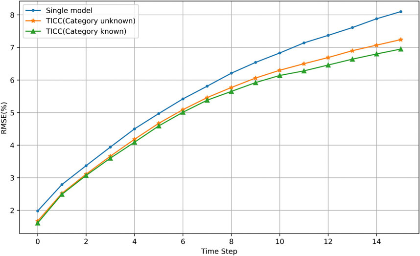
FIGURE 9. The prediction results of TICC method.

The Comparison of Different Regime Division Methods

There are other related regime division methods for wind power prediction. So we compare our method with the other methods (Hu et al., 2014; Xiong et al., 2016). The wind power on the test set is as follows.

As we can see from Figure 10, by using the proposed regime division method, the prediction accuracy of the wind power can be improved compared to other methods especially on the maximum and minimum point of the wind power. We also compute the statistical results on the testing data set. The results are as follows in Table 2.

TABLE 2

TABLE 2. The prediction results of different regime division methods (%). The minimum of the RMSE and MAE of different prediction time is in bold.

FIGURE 10

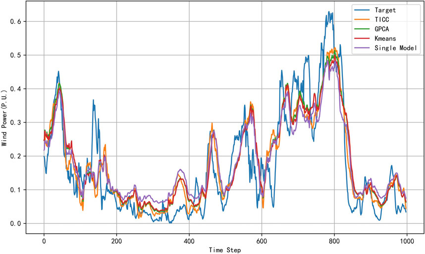
FIGURE 10. The comparison of different regime division methods.

According to the results in Table 2, we can see that the prediction model by the TICC regime division method performs better than other models.

Conclusion

In this paper, an ultra-short-term wind power prediction method is proposed based on the Markov regime switching model. We cluster the operation states of the wind farms according to the historical wind power, historical NWP information and future wind power. The following conclusions can be reached.

(1) The operation state of the wind farms is a high dimension vector. But it can be represented by a much lower dimension vector due to the graph autoencoder. It can avoid the dimension disaster problem in the pattern division part.

(2) The operation state of the wind farms can be divided into several regimes. By reasonable regime division and designing a prediction model separately for each regime, the prediction accuracy can be increased.

(3) The TICC method can consider the spatiotemporal relationship of the wind farm operation state. Therefore, the prediction accuracy of TICC is much higher than the other regime division methods which don’ take consider the spatiotemporal relationship.

Data Availability Statement

The datasets presented in this article are not readily available because The data is provided by the State Grid Corporation in China and there is strict limitation for the use of those data. So those data cannot be shared due to the privacy problem. Requests to access the datasets can be directed to fanhang123456@163.com and we can help to contact the owner of the dataset.

Author Contributions

HF, XZ, and JZ contributed conception and design of the study. HF performed the data analysis and wrote the first draft. XZ, SM, and JZ helped to revise the manuscript. All authors approved the submitted version.

Funding

This work is supported by National Key R&D Program of China (Technology and application of wind power/photovoltaic power prediction for promoting renewable energy consumption, 2018YFB0904200) and eponymous Complement S&T Program of State Grid Corporation of China (SGLNDKOOKJJS1800266).

Conflict of Interest

The authors declare that the research was conducted in the absence of any commercial or financial relationships that could be construed as a potential conflict of interest.

References

Boyd, S., Parikh, N., and Chu, E. (2011). Distributed optimization and statistical learning via the alternating direction method of multipliers. Hanover, MA: Now Publishers Inc.

Demolli, H., Dokuz, A. S., Ecemis, A., and Gokcek, M. (2019). Wind power forecasting based on daily wind speed data using machine learning algorithms. Energy Convers. Manag. 198, 111823. doi:10.1016/j.enconman.2019.111823

CrossRef Full Text | Google Scholar

Duong, M. Q., Grimaccia, F., Leva, S., Mussetta, M., and Le, K. H. (2015). Improving transient stability in a grid-connected squirrel-cage induction generator wind turbine system using a fuzzy logic controller. Energies 8 (7), 6328–6349. doi:10.3390/en8076328

CrossRef Full Text | Google Scholar

Duong, M. Q., Grimaccia, F., Leva, S., Mussetta, M., and Ogliari, E. (2014). Pitch angle control using hybrid controller for all operating regions of SCIG wind turbine system. Renew. Energy 70, 197–203. doi:10.1016/j.renene.2014.03.072

CrossRef Full Text | Google Scholar

Duong, M. Q., Ogliari, E., Grimaccia, F., Leva, S., and Mussetta, M. (2013). “Hybrid model for hourly forecast of photovoltaic and wind power,” in IEEE International Conference on Fuzzy Systems (FUZZ-IEEE), Hyderabad, India, July 7–10, 2013 (IEEE), 1–6. doi:10.1109/FUZZ-IEEE.2013.6622453

CrossRef Full Text | Google Scholar

Fan, H., Zhang, X., Mei, S., Chen, K., and Chen, X. (2020). M2GSNet: multi-modal multi-task graph spatiotemporal network for ultra-short-term wind farm cluster power prediction. Appl. Sci. 10, 7915. doi:10.3390/app10217915

CrossRef Full Text | Google Scholar

Feng, S. L., Wang, W. S., Liu, C., and Dai, H. Z. (2010). Study on the physical approach to wind power prediction. Proc. CSEE 30, 1–6. doi:10.13334/j.0258-8013.pcsee.2010.02.014

CrossRef Full Text | Google Scholar

Goodfellow, I., Bengio, Y., Courville, A., and Bengio, Y. (2016). Deep learning. Cambridge, MA: MIT Press.

Hallac, D., Vare, S., Boyd, S., and Leskovec, J. (2017). “Toeplitz inverse covariance-based clustering of multivariate time series data,” in KDD’17: Proceedings of the 23rd ACM SIGKDD International Conference on Knowledge Discovery and Data Mining, Halifax, Canada, August, 2017 (New York, NY: Association for Computing Machinery), 215–223. doi:10.1145/3097983.3098060

CrossRef Full Text | Google Scholar

Hamilton, J. D. (1989). A new approach to the economic analysis of nonstationary time series and the business cycle. Econometrica 57, 357–384.

CrossRef Full Text | Google Scholar

Hu, Q., Su, P., Yu, D., and Liu, J. (2014). Pattern-based wind speed prediction based on generalized principal component analysis. IEEE Trans. Sust. Energy 5, 866–874. doi:10.1109/TSTE.2013.2295402

CrossRef Full Text | Google Scholar

Huang, G. B., Zhu, Q. Y., and Siew, C. K. (2006). Extreme learning machine: theory and applications. Neurocomputing 70, 489–501. doi:10.1016/j.neucom.2005.12.126

CrossRef Full Text | Google Scholar

Jiang, Y., Song, Z., and Kusiak, A. (2013). Very short-term wind speed forecasting with Bayesian structural break model. Renew. Energy 50, 637–647. doi:10.1016/j.renene.2012.07.041

CrossRef Full Text | Google Scholar

Khodayar, M., and Wang, J. (2018). Spatio-temporal graph deep neural network for short-term wind speed forecasting. IEEE Trans. Sust. Energy 10, 670–681. doi:10.1109/TSTE.2018.2844102

CrossRef Full Text | Google Scholar

Kou, P., Gao, F., and Guan, X. (2013). Sparse online warped Gaussian process for wind power probabilistic forecasting. Appl. Energy 108, 410–428. doi:10.1016/j.apenergy.2013.03.038

CrossRef Full Text | Google Scholar

Lai, G., Chang, W. C., Yang, Y., and Liu, H. (2018). “Modeling Long- and short-term temporal patterns with deep neural networks”, in Proceedings of the 41st international ACM SIGIR conference on research AND development in information retrieval, Ann Arbor, MI, July, 2018 (New York, NY: Association for Computing Machinery). doi:10.475/123_4

CrossRef Full Text | Google Scholar

Lavielle, M., and Lebarbier, E. (2001). An application of MCMC methods for the multiple change-points problem. Signal. Process. 81, 39–53. doi:10.1016/S0165-1684(00)00189-4

CrossRef Full Text | Google Scholar

Lee, J., Zhao, F., Dutton, A., et al. (2020). Global wind report 2019. Brussels, Belgium: Global Wind Energy Council.

Liu, Y., Tajbakhsh, S. D., and Conejo, A. J. (2020). Spatiotemporal wind forecasting by learning a hierarchically sparse inverse covariance matrix using wind directions. Int. J. Forecast. doi:10.1016/j.ijforecast.2020.09.009

CrossRef Full Text | Google Scholar

Messner, J. W., and Pinson, P. (2019). Online adaptive lasso estimation in vector autoregressive models for high dimensional wind power forecasting. Int. J. Forecast. 35, 1485–1498. doi:10.1016/j.ijforecast.2018.02.001

CrossRef Full Text | Google Scholar

Murphy, K. P. (2012). Machine learning, a probabilistic perspective. Cambridge, MA: MIT Press, 27, 62–63.

Park, J. M., and Kim, J. H. (2017). “Online recurrent extreme learning machine and its application to time-series prediction”, in 2017 International Joint Conference on Neural Networks (IJCNN), Anchorage, AK, May 14–19, 2017 (New York, NY: IEEE), 1983–1990. doi:10.1109/IJCNN.2017.7966094

CrossRef Full Text | Google Scholar

Pedregosa, F., Varoquaux, G., Gramfort, A., Michel, V., Thirion, B., Grisel, O., et al. (2011). Scikit-learn: machine learning in Python. J. machine Learn. Res. 12, 2825–2830.

Google Scholar

Peng, X. S., Xiong, L., Wen, J. Y., Cheng, S. J., Deng, D. Y., Feng, S. L., et al. (2016). A summary of the state of the art for short-term and ultra-short-term wind power prediction of regions. Proc. CSEE 36, 6315–6325. doi:10.13334/j.0258-8013.pcsee.161167

CrossRef Full Text | Google Scholar

Smith, A., Naik, P. A., and Tsai, C. L. (2006). Markov-switching model selection using Kullback–Leibler divergence. J. Econom. 134 (2), 553–577. doi:10.1016/j.jeconom.2005.07.005

CrossRef Full Text | Google Scholar

Song, Z., Jiang, Y., and Zhang, Z. (2014). Short-term wind speed forecasting with Markov-switching model. Appl. Energy 130, 103–112. doi:10.1016/j.apenergy.2014.05.026

CrossRef Full Text | Google Scholar

Sun, M., Feng, C., and Zhang, J. (2020). Multi-distribution ensemble probabilistic wind power forecasting. Renew. Energy 148, 135–149. doi:10.1016/j.renene.2019.11.145

CrossRef Full Text | Google Scholar

Wang, R., Li, C., Fu, W., and Tang, G. (2020). Deep learning method based on gated recurrent unit and variational mode decomposition for short-term wind power interval prediction. IEEE Trans. Neural Netw. Learn. Syst. 31, 3814–3827. doi:10.1109/TNNLS.2019.2946414

PubMed Abstract | CrossRef Full Text | Google Scholar

Wytock, M., and Kolter, Z. (2013). “Sparse Gaussian conditional random fields: algorithms, theory, and application to energy forecasting,” in Proceedings of the 30th International Conference on Machine Learning, Atlanta, GA, June, 2013, 28, 1265–1273.

Google Scholar

Xiong, Y., Liu, K., Qin, L., Ouyang, T., and He, J. (2019). Short-term wind power prediction method based on dynamic wind power weather division of time sequence data. Power Syst. Technol. 43, 3353–3359. doi:10.13335/j.1000-3673.pst.2018.1568

CrossRef Full Text | Google Scholar

Xiong, Y., Zha, X., Qin, L., Ouyang, T., and Xia, T. (2016). Research on wind power ramp events prediction based on strongly convective weather classification. IET Renew. Power Gener. 11, 1278–1285. doi:10.1049/iet-rpg.2016.0516

CrossRef Full Text | Google Scholar

Xue, Y., Yu, C., Zhao, J., Li, K., Liu, X., Wu, Q., et al. (2015). A review on short-term and ultra-short-term wind power prediction. Automation Electric Power Syst. 39, 141–151. doi:10.7500/AEPS20141218003

CrossRef Full Text | Google Scholar

Zhao, Y., Ye, L., Pinson, P., Tang, Y., and Lu, P. (2018). Correlation-constrained and sparsity-controlled vector autoregressive model for spatio-temporal wind power forecasting. IEEE Trans. Power Syst. 33, 5029–5040. doi:10.1109/TPWRS.2018.2794450

CrossRef Full Text | Google Scholar