Investigating the Effect of Cloud Cover on Radiative Cooling Potential With Artificial Neural Network Modeling

Radiative cooling is a novel and promising technology in which, heat is radiated through the infrared wavelength (8–13 μm) to the cold outer space, while the incident solar radiation (0.3–4 μm) is reflected. This leads to a temperature reduction in the material that can be utilized as a free and renewable resource of cooling for different applications. For the sake of increasing the efficiency and the cooling potential of these systems, scientists have precisely studied the affecting parameters and developed analytical equations. The sky cloud coverage is one of the major affecting parameters that is challenging to model due to its inherent complexity and diversity. Therefore, in this article, we investigated the effect of cloud cover on the radiative cooling potential by utilizing machine learning techniques. In this regard, a non-linear autoregressive with exogenous feedback (NARX) neural network has been developed to predict the temperature of the system in different climate conditions by taking cloud coverage into account. Results of this investigation indicate that there is an intensely indirect relationship between cloud coverage and the performance of the system. Accordingly, a cloudy sky can lead to 15°C inaccuracy in the modeling of the system and may even lead to a temperature increase relative to the ambient, which inhibits the applicability of the system. It was eventually concluded that the cloud cover, as one of the major parameters that determine the performance of the system, must be taken into account in radiative cooling system designs.

Introduction

Cooling is regarded as a crucial end-use of energy in the world as well as a key driver of the maximum electricity demand (Raman et al., 2014). It is believed that, globally, cooling systems are responsible for the consumption of 15% of the generated electricity and also 10% of the released greenhouse gas. It is estimated that the demand for cooling energy can grow up to 1000% by 2050 (Goldstein et al., 2017). Therefore, given that the radiative cooling strategy can help cool the devices without any electricity input, they can have a substantial impact on global energy consumption (Raman et al., 2014). Unlike the dominant cooling methods, the radiative cooling system which is a natural cooling method requires no input energy to cool itself (Zhai et al., 2017). Radiative cooling refers to a passive cooling technique that decreases the temperature of the object below the ambient air. For this purpose, a specific device should be placed toward the sky in order to radiate its heat to the outer space through a transparent window within 8 to 13 micrometers (Raman et al., 2014). Nevertheless, it is necessary to provide materials that can radiate intense thermal energy and absorb the least possible solar radiation. Although the majority of the cooling demand is requested during the day, such radiative cooling has been mainly used during dry and clear nights; besides, it only has restricted application in commercial refrigeration and air conditioning systems. Since the radiative cooling requires both high thermal radiation and high solar reflection during the day, it is challenging to achieve a lower temperature than diurnal ambient temperature. Photonic materials have recently been developed in a way that they can perfectly emit their heat to the outer space and operate at a temperature below the ambient under direct sunlight (Goldstein et al., 2017). This new generation of radiative cooling systems are capable of emitting a great amount of radiation in the transparent windows, and meanwhile, reflecting abundantly within the target solar emission band (0.3 – 4.0 μm). Hence, these devices can provide significant radiative cooling during the day (Zhao et al., 2019a). Given those radiative cooling systems that can help freely reduce the temperature in the enclosed areas and cool the outer surfaces, they have been applied in the roofs and the facades of the buildings or the cooler fluids. They can also be implemented to reduce the temperature in a fluid media during the night which can be stored for cooling purposes during the next days or can be consumed directly (Lu et al., 2016; Zuazua-Ros et al., 2017; Phys et al., 2019; Yuan et al., 2020). Moreover, these systems might be able to cool the photovoltaic panels (Siecker et al., 2017). The related literature suggests that some researchers have conducted different studies on radiative cooling in a variety of scientific journals that are pertinent to energy consumption; the following section entails a summary of some of such studies.

Goldstein et al. (2017) conducted a study on cooling water below the air temperature without electricity by employing the daytime radiative cooling technique. They fabricated the aforementioned system including polyethylene cover as a radiative cooling material, a heat exchanger, and polystyrene insulation. The results have shown that given the heat rejection rate up to 70 W/m² in a total surface area of 0.74 m², the radiative cooling can cool the water up to 5°C below the ambient temperature, provided that the water flow rate is equal to 0.21 L/min.m². Moreover, they demonstrated that the integration of this system into the conventional cooling systems of a building can help to reduce the cooling energy consumption by up to 21%.

Zhao et al. (2019b) carried out a study to develop a radiative cooling system in order to decrease water temperature during the day and the night. The researchers also analyzed the effect of weather conditions on the radiative cooling performance and concluded that the radiative cooling system can produce a cooling power of 1.29 kW and 607 W during the night and day, respectively. Moreover, it cools water up to 10.6°C below the ambient temperature at noon. Besides, Yuan et al. (2020) utilized a spectral selective polymer-based meta-material on top of an aluminum container including water to compare the performance of this system with bare aluminum plate and aluminum foil covered plate. The results demonstrated that the meta-material element can maintain the water temperature 2–14 °C below the air temperature by employing a radiative sky cooling mechanism. Zhao et al. (2019b) proposed a study in the PV-RC systems. They presented a novel approach of the hybrid photovoltaic panel and nocturnal radiative cooling to generate electricity and obtain cooling energy. The experimental setup was carried out in China. The result demonstrated that the electrical efficiency is 12.4% along with an average energy output of 75 W/m² and the temperature was reduced to 12.7°C below the ambient temperature for the nocturnal RC process.

Hu et al. (2017) proposed a combined photovoltaic (PV), photothermic (PT), and nocturnal radiative cooling (RC) that generate electricity and heat during the daytime using PV and PT and cooling energy at nighttime with employing RC. Moreover, not only a sensitivity analysis is conducted but also an experimental setup was utilized to estimate the daily solar heating and RC performance. The result revealed that insulation thickness and ambient temperature have a positive effect on cooling performance, whereas precipitable water vapor, wind, and velocity have a negative impact on cooling performance.

It should be noted that the radiative cooling performance mechanism can be affected by a variety of factors such as cloud coverage, air temperature, solar radiation, type of materials, dew point temperature, and wind speed. Different approaches are used to investigate the effectiveness of these parameters which are applied through sensitivity analysis and experimental set-up. however, the excessive costs of these set-ups (Alnaqi et al., 2019) and failure to develop an accurate equation to investigate the impact of cloud cover have imposed great difficulties in predicting the probable values (it is noteworthy that all of these factors are precisely taken into account in the proposed equations except for cloud coverage). In this regard, the researchers are motivated to propose predicting models using statistical/numerical approaches. Accordingly, different data-driven approaches [e.g., artificial neural network (ANN)] can provide more appropriate scales.

ANN is regarded as a forecasting method to determine the desirable functions (Alnaqi et al., 2019). It is believed that ANN can provide a different approach to deal with poorly defined and also complicated issues. These networks can tolerate deficiencies because they are capable of managing imperfect and noisy data, can handle nonlinear problems, can take advantage of the examples, and can carry out the forecast and also generalization at maximum pace. They are also implemented in a variety of applications in the areas of medicine, optimization, control, signal processing, power systems, social/psychological sciences, forecasting, manufacturing, pattern recognition, and robotics.

ANN is a combination of smaller interlocked processing units that transmit the information through interconnections. The input values as well as the weight values are associated with an incoming connection. Therefore, the combined values are regarded as the output value in these units. Due to the acquisition-based nature of the ANNs, they should be trained in a way to observe and discover the proposed patterns according to the available data sets. Consequently, ANNs are utilized to analyze the new patterns for categorization and estimation. It is believed that ANNs are more appropriate for the tasks comprising incomplete and fuzzy information or datasets as well as complicated and improper problems. ANNs are capable of learning from the available empirical data, hence, they can resolve non-linear problems as well. Moreover, ANNs can bear with the errors and they show strength and vigor. Thus, they can be applied to a wide range of application fields (Kalogirou, 2001). Recently, researchers have indicated the appropriate implementation of ANNs in terms of processing patterns and modeling pertinent to solar energy.

According to the ANN model with fuzzy logic pre-processing, the solar estimating algorithm was developed by Sivaneasan et al. (2017). For this purpose, they used the tangent sigmoid function as the transfer function as well as the Levenberg-Marquardt optimization approach in the neural network.

A PVT control algorithm was developed by Ammar et al. (2013) using an ANN for detection of the Optimal Power Operation Point (OPOP). The OPOP is used to determine the optimum mass flow rate of the PVT for ambient temperature and continuous radiation power. Intending to investigate different PVT systems, Al-waeli et al. (2018) utilized a Multi-Layer Perceptron (MLP) system based on ANN including Nanofluid/Nano Phase change material (PCM), conventional PV, water-based photovoltaic-thermal (PVT), and water-Nano fluid PVT. It is also noteworthy that the tests are applied in the same environment and conditions. Besides, they also used a three-ANN approach (including MLP, Support Vector Machine, & Self-Organizing Feature Mapping methods) to estimate the electrical current and efficiency of the PV panels in a Nano-fluid-cooled and Nano-PCM cooled PVT system. They concluded that such a well-trained network can have satisfactory performance. Besides, A. Mashaly and A. Alazba (Mashaly and Alazba, 2016) investigated the thermal productivity of a solar still using the two models of multiple linear regressions (MLR) and Multi-Layer Perceptron (MLP) neural networks. Weather and other affective variables such as wind speed, relative humidity, ambient temperature, and the other six parameters are regarded as the input variables and then the thermal efficiency is presented as the output layer. The results indicated that the MLP model could have a better performance assessment compared to the MLR model.

Moreover, Huang et al. (2016) decided to evaluate the power output of photovoltaic panels through an ANN. They also further included the solar peak angle and solar azimuth angle to the environmental factors as the algorithm input. They concluded that the proposed ANN model can greatly improve the efficiency of long-run predictions in different weather conditions. Ceylan et al. (2014) foretold the photovoltaic module temperature using an ANN in Turkey based on the solar radiation and air temperature as the input variables. They also regarded module temperature as the output variable for the training process of ANN.

Similarly, Icel et al. (2019) also used the ANN models to predict the power which is generated by the PV panels located in three cities in Turkey. The following input parameters were identified using the proposed ANN models: humidity rate, air temperature, photovoltaic module temperature, wind velocity, and solar irradiance. The PV panel power prediction was successful for three different cities in 99% of the cases.

In another study, Citakoglu (2015) attempted to propose a model for monthly solar radiation values using MLR and ANN techniques. Then, they developed an MLR model to examine the ANN performance. It is also believed that, as an ANN model, the MLP network has called for great efforts in resolving different problems. Under composite climatic conditions, Perveen et al. (2020) developed an ANN model for the prediction of short-term power in a solar system using 210W polycrystalline PV panels. As a result, cell temperature, solar radiation, short circuit, and open-circuit voltage were identified as input parameters in the ANN model. This research indicated that the proposed ANN model is capable of achieving better performance, comparing to other networks within the acceptable limits. Therefore, ANN can be regarded as an appropriate approach to predict the weather parameters under various working conditions. Furthermore, Rocha et al. (2020) proposed three different ANN models to evaluate the power generation of a 3 kW solar power plant in diverse locations. The models were performed at different intervals such as 5 min, 10 min, and 1 h. However, they only used ambient temperature data and irradiance as the input parameter of ANN in their study.

It is necessary to provide a precise and reliable estimation of the total cloud cover (TCC) for different areas such as energy demand and production, agriculture, as well as astronomy. Most meteor-logical centers investigate ensemble calculations of TCC; nevertheless, these forecasts are often miss-calibrated and show the worse forecast skill compared to ensemble forecasts of other weather variables. Hence, it is necessary to apply post-processing models to improve predictive performance (Lerch and Ayari, 2020). It is also noticeable that reliable and accurate prediction of TCC has major importance in the prediction of radiative sky cooling performance (Zhao et al., 2019b).

In the present study, a hybrid meta-material thin film (Zhao et al., 2019b) which is made of glass-polymer was used because of its potential to produce 93 W/m² radiative cooling power under direct sunlight at noon. This meta-material includes a translucent polymer that can cover the entire solar continuum. Moreover, it consists of silicon dioxide (SiO₂) microspheres which are dispersed randomly. Given the phonon-evolved Frohlich radiations of the fixed microspheres, the meta-materials are excessively emissive throughout the whole atmospheric diffusion window (i.e. infrared wavelength of 8–13 μm). As a result, the present study has proposed a set of radiative cooling modules through the implementation of glass-polymer hybrid meta-material.

Moreover, a review of the related literature showed that there is no evidence on the application of ANN to predict the effects of cloud cover on the radiative cooling performance. It is noteworthy that the present study is the very first study to investigate the aforementioned effects. Therefore, the present study aims to fill this gap through an evaluation of the post-processing performance using the nonlinear autoregressive network with exogenous input (NARX) neural networks method. We attempt to build a non-linear relationship between the temperature changes of the radiative cooling system and the effective parameters for the city of Boulder which is located in the north of Colorado State. In this regard, the NARX method is proposed to observe the changes in the temperature of the radiative cooling system. For this purpose, five input layers, which affect the changes in the temperature of the radiative cooling system were used to form the dataset including ambient temperature, solar radiation, wind speed, precipitable water vapor, and cloud cover.

Materials and Methods

Figure 1 shows the constituent layers of the studied radiative cooling system. At the top of the radiative cooling, there is a 50-micron layer of polymeric material that is responsible for the emittance of the heat from the radiative cooling to outer space. Then, there is a 200-nanometer layer of silver which reflects the incoming solar radiation to the outside. An adhesive layer also holds the components on a polycarbonate container that comprises water. And ultimately, in the bottom section, there is a volume of water that is supposed to be cooled.

FIGURE 1

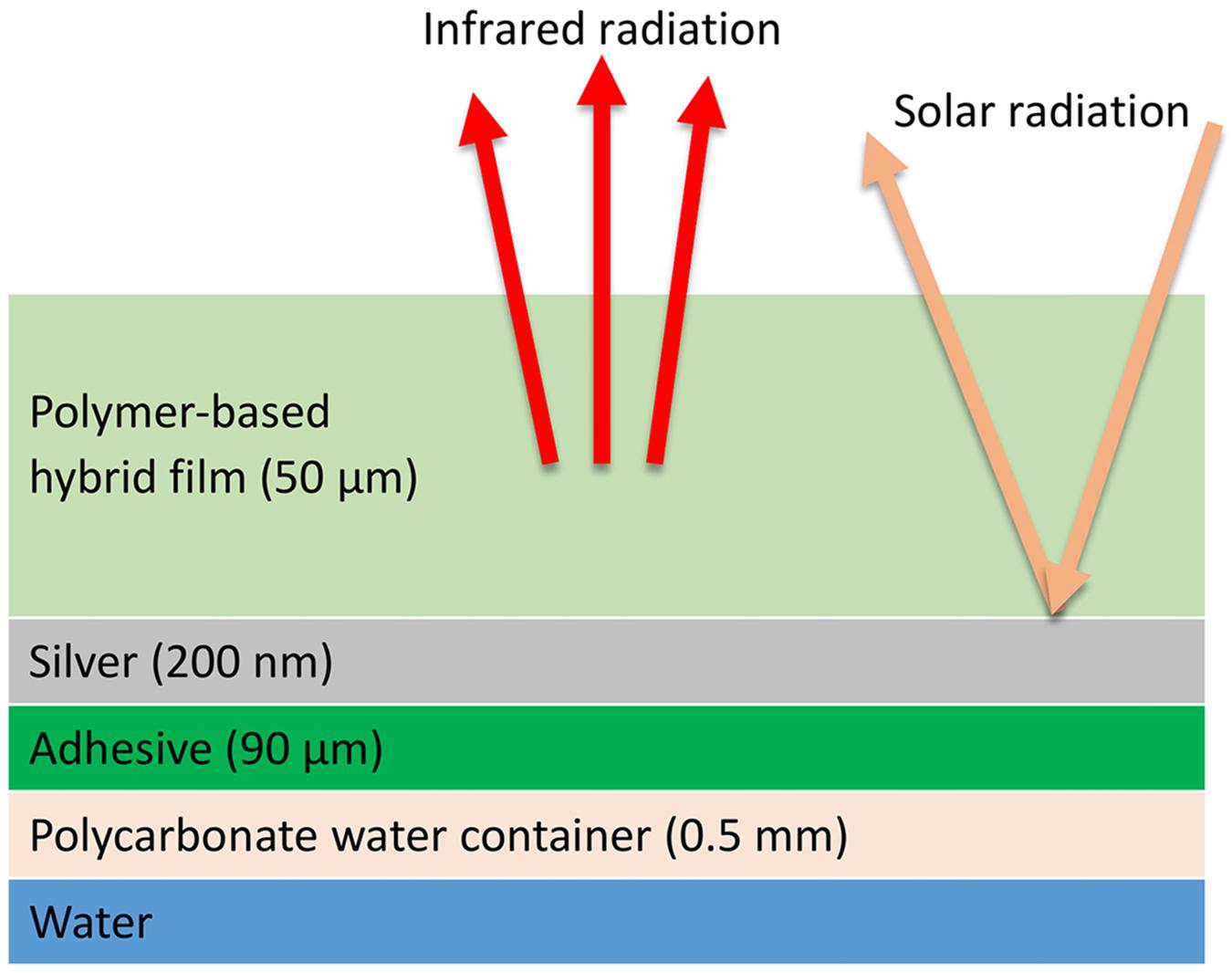
Figure 1. Position of layers in the radiative cooling system.

Figure 2 illustrates the emissivity of the examined radiative cooling material along with the solar irradiation. Accordingly, the solar radiation is within the wavelengths of 0.3 to about 3 microns, in which the emissivity/absorptivity coefficients of the radiative cooling system are approximately 0.04 (Zhao et al., 2019a). In other words, about 96% of the incoming radiation to the radiative cooling is reflected and only a small proportion of this radiation is absorbed by the radiative cooling. On the other hand, the radiation of the terrestrial objects occurs within the range of 8 to 13 microns, and according to Figure 2, the emissivity/absorptivity of the radiative cooling is approximately 0.9 in this range. Therefore, terrestrial objects can dissipate a large part of their heat into outer space. This creates a net heat flux from the radiative cooling to outer space. As a result, despite being in direct sunlight, the temperature of the radiative cooling will be lower than the ambient. Figure 3 indicates the components of the cooling system. The radiative cooling system and the water container is surrounded by layers of polyisocyanurate thermal insulation to minimize the conductive heat dissipation from the sides and bottom. A layer of polyethylene is placed on top of the apparatus to reduce the effect of wind on the net power of the system. Given the high transmittance of polyethylene, it does not interfere with the cooling capacity of the system (Boriskina, 2019). A thin layer of air between the polyethylene layer and the material also acts as a thermal insulator. The apparatus is placed with a 15° incline to the north to reduce the solar radiation and facilitate the water pouring process. Table 1 shows the dimensions of these components.

FIGURE 2

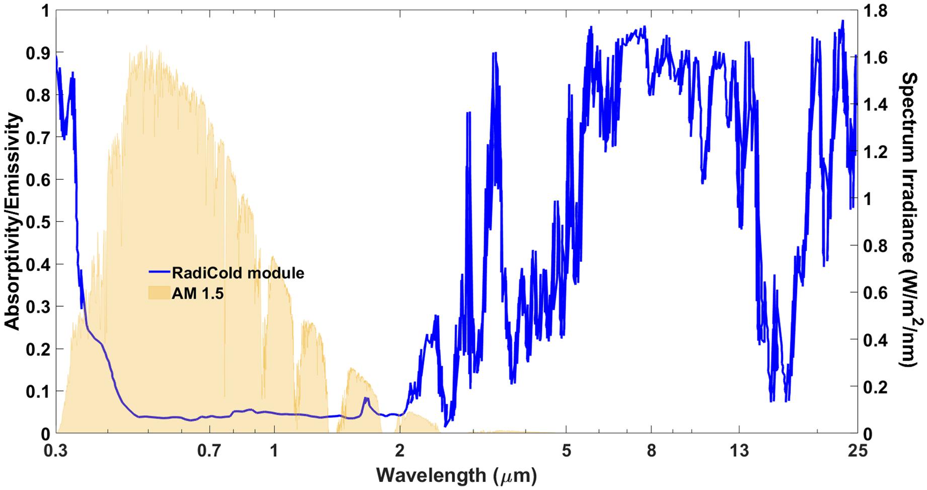
Figure 2. Wavelength-dependent emissivity of the radiative cooling system (RadiCold) along with the AM 1.5 solar spectrum.

FIGURE 3

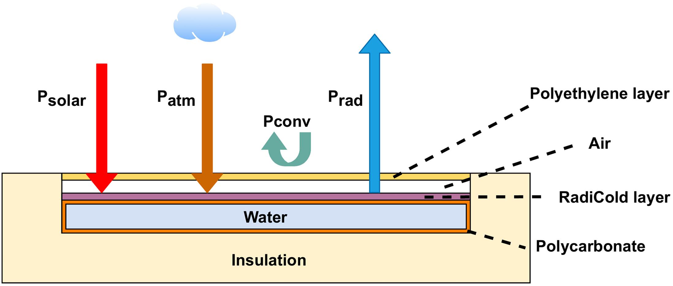
Figure 3. Components of the radiative cooling system with heat flows.

TABLE 1

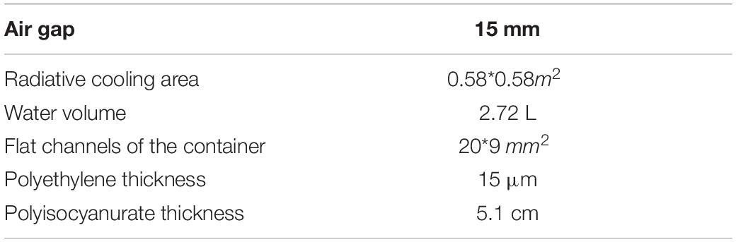
Table 1. Dimensions of the system components.

Artificial Neural Networks

The cloud cover affects the radiative cooling of the system and also the solar radiation as well as the atmospheric radiation. Therefore, it is unlikely to establish an explicit correlation between cloud coverage and net radiative cooling power. Artificial neural networks can be beneficial to understand the effect of cloud cover on radiative cooling power and consequently, on the radiative cooling temperature. In this regard, a neural network can be trained by providing a database of geographical parameters, including cloud cover to obtain the temperature of the material and water. Therefore, based on different cloud cover coefficients between 0 for a clear sky and 1 for a completely cloudy sky, the temperature of the system can be predicted.

The calculation of radiative cooling temperature is inherently dependent on its temperatures in the previous times, and also due to the delays in temperature changes, meteorological data must enter the neural network with their values previous in the past. Therefore, using a recursive neural network to calculate the temperature will yield far better results compared to other types of neural networks. This neural network is implemented in MATLAB as a nonlinear autoregressive network with exogenous inputs (NARX) that has input and output data with a specified amount of delay into the neural network (Siegelmann et al., 1997). The inputs of this neural network are: ambient temperature (T_amb), solar radiation (G_solar), wind speed (V), precipitable water vapor (W), and cloud cover coefficient (β), which are obtained by the meteorlogic stations in Boulder (Andreas and Stoffel, 1981). Finally, the temperature of the system at the examination moment is calculated by the output value of the neural network. In this neural network, there is no need to enter the data with delay as well as extracted feedback from the output manually because the applied neural network has a closed-loop structure.

In the context of training algorithm, by evaluating the different existing training algorithms (e.g., Levenberg-Marquardt, Bayesian Regularization, and Scaled Conjugate Gradient), the Levenberg-Marquardt has obtained lower errors with an acceptable convergence speed in most of the examinations. Therefore, the Levenberg-Marquardt, which is a great method to solve nonlinear parameter estimation problems has been utilized in for this problem. Figure 4 demonstrates the main components of the developed neural network. This neural network consists of 5 neurons in the input layer, 27 neurons in the hidden layer that contain input data along with their latencies as well as the feedback with delays from the output, and 1 neuron in the output layer. The applied transfer function in the hidden layer is a sigmoid tangent, which is suitable for the simulation of the radiative cooling phenomenon. The output layer also has a linear transfer function to directly display the output value. The performance of this neural network is also calculated by the Mean Squared Error (MSE), which takes into account both the variance and bias values of the obtained responses.

FIGURE 4

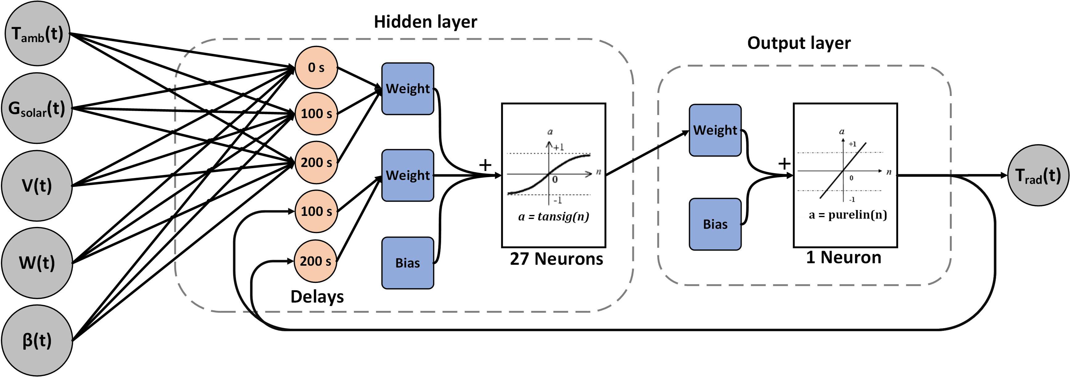
Figure 4. Structure of the NARX neural network for predicting the temperature of the system and water.

The output value of a neural network with input, hidden, and output layers is shown in Eq. 1. According to this relationship, y_i,hidden, which represents the i^th output of m^thneuron in the hidden layer is multiplied by the corresponding weight in the output layer ($W^{\prime }{}_i$) and is then summed with a constant bias value in the output layer ($B^{\prime }{}_{\text{out}})$. Then, the obtained values are multiplied by the output layer transfer function (f_out) which is calculated by Eq. 3. Finally, the obtained output (y_out) shows the output value of the neural network which is the temperature of the system (T_film). It should also be noted that, the i^ththeoutput of the hidden layer (y_i,hidden) is obtained by Eq. 2. In this equation, the j^th the input of the neural network (x_j,input) is multiplied by the weight of the j^th input of the n^th neuron (W_i,j). After aggregating these values, they are summed with the bias value of the i^th neuron (B_i,hidden). Ultimately, the output of the hidden layer for each neuron is obtained by multiplying the calculated values with the transfer function used in the hidden layer (f_hidden), which is determined by Eq. 4.

$$y_{out}=f_{out}(\sum _{i=1}^m{y}_{i,hidden}W^{\prime }{}_i+B^{\prime }{}_{out})(1)$$

$$y_{i,hidden}=f_{hidden}(\sum _{j=1}^n{x}_{j,input}{W}_{i,j}+B_{i,hidden})(2)$$

Eqs. 3, 4 represent the transfer functions used in each layer of the neural network. According to Eq. 3, the output layer transfer function (f_out(x)) is a linear function (purelin(x)). The input data from the hidden layer is aggregated after applying weights and biases and it comes out from the corresponding layer without applying any changes. Afterward, the output value is obtained. The hidden layer transfer function (f_hidden(x)) is sigmoid, which is given in Eq. 4. This transfer function, which is widely used in various neural networks, makes a great deal of adaptation to real data.

$$f_{out}\left(x\right)=purelin\left(x\right)=n(3)$$

$$f_{hidden}\left(x\right)=tansig\left(x\right)=\frac{2}{1+\exp \left(-2x\right)}-1(4)$$

Eq. 5 shows the output value of the neural network based on different input values. In this equation, x_input(t)refers to the input of the neural network at the time (t), which is calculated by Eq. 6. Based on the time steps in the database, latencies used in this neural network for the input and output feedbacks are 100 and 200 s, respectively. This equation states that the temperature of the system depends on the climatic parameters at the time (t), 100 and 200 s before the time (t), as well as the its temperature at 100 and 200 s before that time.

$$y_{out}\left(t\right)=T_{film}\left(t\right)=f(x_{input}\left(t\right)+x_{input}(t-100)\mathrm{\hspace{1em}}+x_{input}\left(t-200\right)+T_{film}\left(t-100\right)+T_{film}(t-200)(5)$$

$$x_{input}\left(t\right)=T_{amb}\left(t\right)+G_{solar}\left(t\right)+V\left(t\right)+W\left(t\right)+\mathrm{\beta }\left(t\right)(6)$$

To evaluate the performance of the neural network, the Mean Squared Error (MSE) function is employed which is expressed by Eq. 7. In this equation, y_i,out is the output of the neural network and y_i,target is the target value.

$$MSE=\frac{1}{n}\sum _{i=1}^N{\left(y_{i,target}-y_{i,out}\right)}^2(7)$$

Mathematical Model

The mathematical model is utilized to calculate the radiative cooling temperature in clear sky conditions. Here, the mathematical model has been implemented to evaluate its accuracy in cloudy conditions and compare it with ANN model. The summation of input and output energy flows of the system is shown in Eq. 8. In this relation, P_rad represents the radiative power of the system to outer space, P_solar refers to the absorbed solar radiation power by the system, P_atm denotes the gained atmospheric radiation by different gas molecules and aerosol particles, and P_conv stands for the amount of heat that an object loses or gains through convection flow.P_net shows the net power of the system. If this value is positive, it means that the radiative cooling temperature is increasing and if it is negative, it leads to a temperature reduction in the system.

$$P_{net}=P_{solar}+P_{atm}+P_{conv}-P_{rad}(8)$$

Eq. 9 shows the amount of radiation that is emitted from the radiative cooling to the sky. According to this relation, I_BB(T_p,λ) refers to the radiation of a black body which is dependent on temperature and wavelength and is calculated using Eq. 10. In this equation, ε_film(λ,θ) is the emissivity of the radiative cooling material that depends on the wavelength and the angle and τ_PE(λ,θ) is the transmittance of polyethylene layer at the top of the apparatus which is variable by wavelength and the angle.

$$P_{rad}=2\mathrm{\pi }{\int }_0^{\frac{\mathrm{\pi }}{2}}{\int }_0^{\mathrm{\infty }}{I}_{BB}(T_p,\mathrm{\lambda }){\mathrm{\epsilon }}_{film}(\mathrm{\lambda },\mathrm{\theta }){\mathrm{\tau }}_{PE}(\mathrm{\lambda },\mathrm{\theta })sin\mathrm{\theta }cos\mathrm{\theta }\mathit{d}\mathrm{\lambda }\mathit{d}\mathrm{\theta }(9)$$

Eq. 10 shows the amount of black body radiation at different wavelengths in the temperature of T_p. In this equation, h and k is the Planck the Boltzmann universal constants which are equal to 6.626×10⁻³⁴J.s, and 1.381×10⁻²³J/K, respectively. Moreover, c refers to the speed of light in the vacuum which is equal to 2.998×10⁸.

$$I_{BB}(T_p,\mathrm{\lambda })=\frac{2h{c}^2}{{\mathrm{\lambda }}^5[exp\left(\frac{hc}{\mathrm{\lambda }k{T}_p}\right)-1]}(10)$$

Eq. 11 shows the absorbed solar radiation power. In this equation, α_film(λ,φ) is the absorptivity of the radiative cooling material, which is dependent on the wavelength and angle of the incident solar radiation; according to Kirchhoff’s law, it is equal to ε_film(λ,φ). I_solar(λ) refers to the incident solar radiation at the wavelength of λ.

$$P_{solar}=cos\mathrm{\phi }{\int }_0^{\mathrm{\infty }}{\mathrm{\alpha }}_{film}(\mathrm{\lambda },\mathrm{\phi }){\mathrm{\tau }}_{PE}(\mathrm{\lambda },\mathrm{\theta })I_{solar}(\mathrm{\lambda })\mathit{d}\mathrm{\lambda }(11)$$

Eq. 12 shows the gained atmospheric radiation. According to this relation, ε_atm(λ,θ,H₂O) is the emissivity of atmospheric particles that depends on the wavelength as well as the direction and the water content of the atmosphere. Other particles also affect the atmospheric emission coefficient, but due to the predominant effect of H_2O over other parameters, humidity is used as an important factor in the calculation of the atmospheric radiation power (Feng et al., 2020). The wavelength-dependent atmospheric emissivity is being calculated by a simplified curve fitting method (Das and Iqbal, 1987).

$$P_{atm}=2\mathrm{\pi }{\displaystyle {\int }_0^{\frac{\mathrm{\pi }}{2}}}{\displaystyle {\int }_0^{\mathrm{\infty }}}{I}_{BB}(T_{amb},\mathrm{\lambda }){\mathrm{\alpha }}_{film}(\mathrm{\lambda },\mathrm{\theta }){\mathrm{\tau }}_{PE}(\mathrm{\lambda },\mathrm{\theta }){\mathrm{\epsilon }}_{atm}(\mathrm{\lambda },\theta ,H_{2}O)sin\theta cos\theta d\mathrm{\lambda }d\theta (12)$$

The amount of convective heat transfer is calculated by Eq. 13, which depends on the temperature of the material, ambient temperature, and the effect of wind on the system. In this regard, h is the heat transfer coefficient of the radiative cooling which is dependent on the wind speed and the system specifications. Accordingly, if the system is applied in such a way that the temperature of the radiative cooling (T_film) is lower than the ambient temperature, then convective heat transfer will be a negative factor. However, if the temperature of the radiative cooling is above the ambient temperature, then convective heat transfer will be positive and thus, it will help to reduce the temperature of the material. To decrease the convection heat loss in the system, a convection shield is used upon the radiative cooling to prevent the wind from blowing directly into the radiative cooling. It is worth noting that the material which is used as a convection shield should not have a structure that interferes with the radiative cooling process; in other words, it should have high transmittance in the atmospheric range (13–18 μm). Polyethylene is usually used as a low-cost material because it has the least effect on radiant cooling as a convection shield (Phys et al., 2019). Eq. 14 is used to calculate the heat transfer coefficient (h), both with a convection shield and without a convection shield in the structure of the radiative cooling system (Zhao et al., 2019b). Conductive heat loss from the lower and lateral surfaces of the system is minimized by the insulators and therefore is ignored in the equations.

$$P_{conv}=h(T_{film}-T_{amb})(13)$$

$$h=\{\begin{array}{cc}8.3+2.5V\hfill & Withoutconvectionshield\hfill \\ 2.5+2V\hfill & Withconvectionshield\hfill \end{array}(14)$$

After calculating the net power of the system P_net, the temperature of the radiative cooling system and the water temperature can be further calculated. Eq. 15 is utilized to calculate the temperature of the system and water in time steps. In this equation, A, m, and C are regarded as the area, mass, and heat capacity of the component, respectively. Also, Δt is the time interval for the calculation of the temperature.

$$T_{film}\left(t+\mathrm{\Delta }t\right)=T_{film}\left(t\right)\mathrm{\hspace{1em}}+{\displaystyle \frac{A_{film}.P_{net}(t)}{(m_{film}.C_{film}+m_{container}.C_{container})}}.\mathrm{\Delta }t(15)$$

Cloud cover is another major factor that affects the net power radiative cooling. Cloud cover limits the heat exchange between the radiative cooling system and outer space. On the other hand, by appearing in front of sunlight, it can absorb a large part of the solar radiation and as a positive factor, improve the radiative cooling performance. Besides, cloud particles radiate on the system, which depends on the emissivity and the temperature of the cloud. Therefore, due to its complex nature and its diverse types, taking cloud coverage into account in estimating the radiative cooling analyses, makes it difficult to estimate the net radiative cooling power (Vall and Castell, 2017). On the other hand, measurements of cloud cover in the sky are limited to a few weather stations and these measurements usually fail to provide accurate information about the cloud coverages. However, various experimental relations have been proposed to calculate the average atmospheric emissivity concerning cloud cover, as shown in Table 2.

TABLE 2

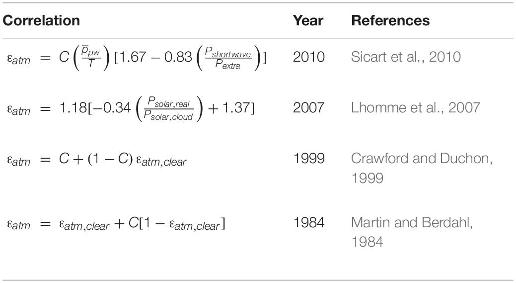
Table 2. Proposed correlations for the average atmospheric emissivity in a cloudy sky.

Results

In this section, the results of the evaluations are represented. First, a mathematical model is required to evaluate the inaccuracy of the modeling in cloudy sky conditions. Therefore, the neural network should be implemented and trained by the empirical data and after evaluating its accuracy, it can be used to predict the performance of the system in different climate conditions.

Validation

The mathematical model is established by the abovementioned equations and needs to be validated by the empirical data to be able to compare the results with the neural network predicted values in cloudy conditions. The experimental data for this system are available for August 28, 2017 as a daytime validation in summer and March 9, 2018 as a nightime validation in winter, which are almost cloudless days (Zhao et al., 2019b). According to Figure 5, the results demonstrated by the proposed model are highly complied with the experimental data, with a maximum error of 0.8°C. For August 28, 2017, the error rates that range from 16:00 onward are slightly higher than the previous hours, which is due to the appearance of scattered clouds in the test area. Therefore, with successful model validation, it can be used to predict the temperature of the system on different days of the year in clear sky conditions.

FIGURE 5

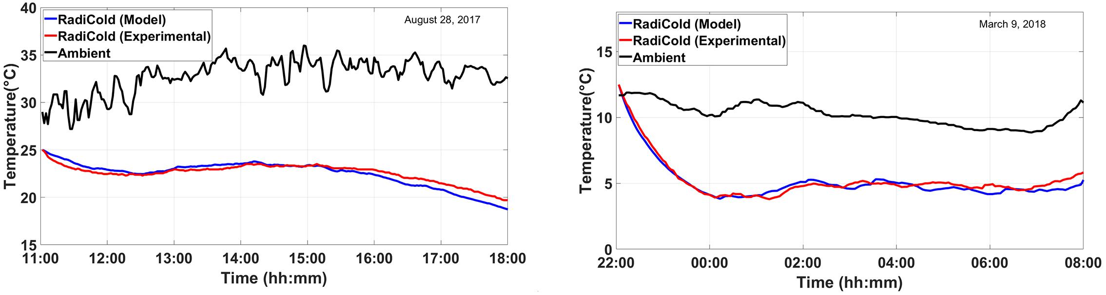
Figure 5. Simulated and experimentally measured radiative cooling temperature (left) in August 28, 2017 and (right) March 9, 2018.

Analyzing the Neural Network

For the sake of training the neural network, radiative cooling experimental data have been utilized on different days of the year and different climate conditions. Figure 6 illustrates the result of the neural network training process, along with climate conditions. These data are modified with a time-step of 200 s to prevent duplicate data from entering the neural network. Ultimately, 1200 data were used to train the neural network that varies between different climatic values. These data have been selected from the hot and cold times of the year to maximize the diversity of the training data and the reliability of the neural network in different conditions. This figure shows the ambient temperature along with the solar radiation variations in this dataset. According to this graph, the ambient temperature for the training dataset varies between 0C and 35C; and the solar radiation varies between 0 and 850 W/m². Besides, the precipitable water vapor values along with changes in wind speed in the region are represented in this figure. According to this figure, the wind speed fluctuates between 0 and 8 m/s, which determines the heat loss due to convective heat transfer. Also, the precipitable water vapor of the region varies between 0.5 and 2 cm. Therefore, a diverse range of atmospheric radiation throughout the year would be obtained. The obtained experimental data by this system, the values predicted by the neural network, and the cloud cover data are represented. Cloud cover for this interval varies between the values of 0.1 (almost clear sky) and 1 (completely cloudy sky). The errors in training this neural network are also shown in this figure. The trained neural network with an average error of 0.00048 and a standard deviation of 0.1976 indicates high accuracy of the trained neural network and can be further used to predict the temperature of the radiative cooling system in different climatic conditions.

FIGURE 6

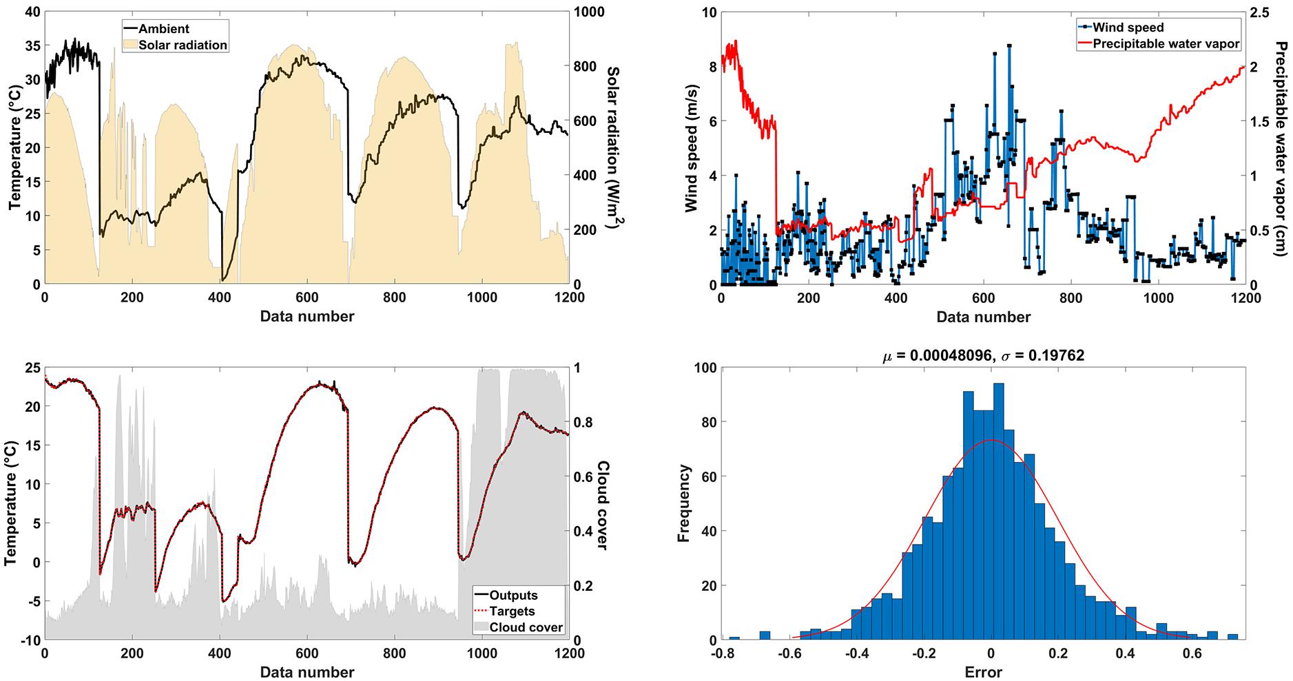
Figure 6. The performance of the ANN model in different climate conditions. (Up-left) the ambient temperature and the solar radiation values versus time (up-right) the wind speed and the precipitable water vapor values of the evaluated points (down-left) output values of ANN and the real target values along with the cloud cover coefficient in the investigated times, and (down-right) the corresponding error histogram.

The designated data are divided into three parts to create this neural network: train, test, and validation data. Train data are applied to train the neural network and determine the weights as well as the biases in each neuron. Validation data is used to prevent overtraining to achieve the best neural network configuration with the specified conditions. Test data are also employed to evaluate neural network performance in predicting objective function. The share of train, validation, and test data is 70%, 15%, and 15%, respectively. Figure 7 shows the results of a comparison between the predicted data and the target data. According to these figures, the results obtained by the neural network with a regression coefficient above 99% for train, validation, and test data indicate that the neural network can be used to predict the temperature of the radiative cooling system.

FIGURE 7

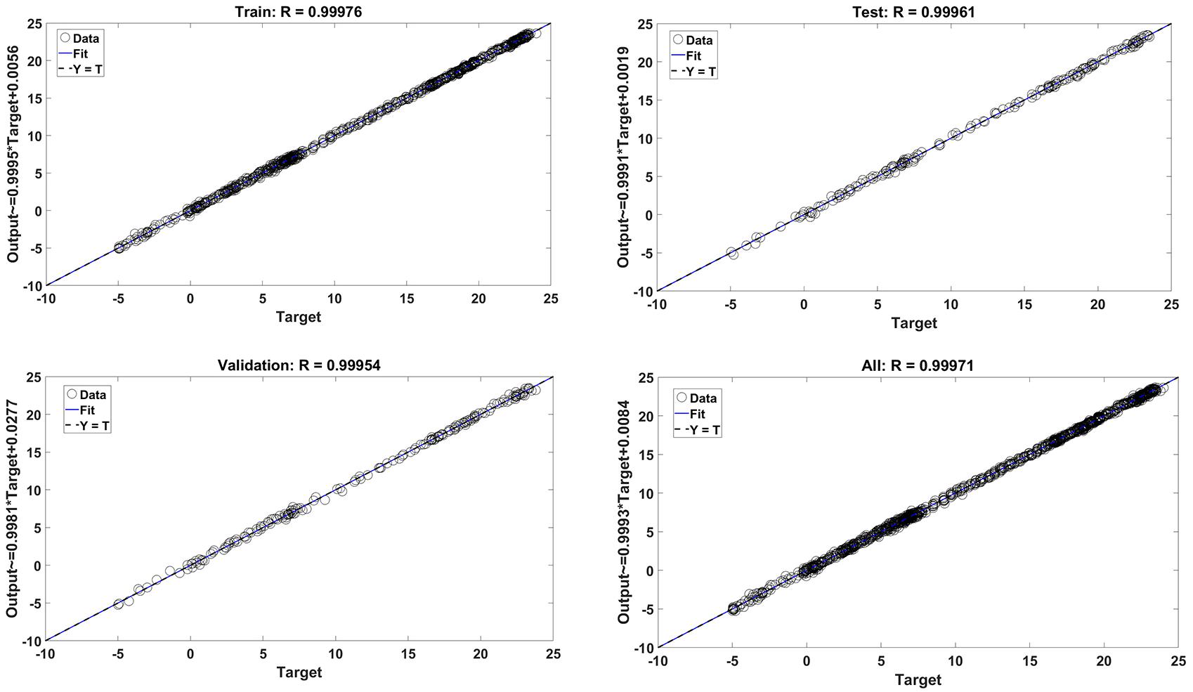
Figure 7. Regression plots of the ANN training process for (Up-left) the training dataset, (up-right) test dataset, (down-left) validation dataset, and (down-right) whole dataset.

To investigate the effect of cloud cover on radiative cooling temperature, the analytical model which was developed for a clear sky was used alongside the experimental data to conceive this temperature difference. The cloud cover data which are gathered by the data collection cameras for February 28, 2018, are shown in Figure 8 (Andreas and Stoffel, 1981).

FIGURE 8

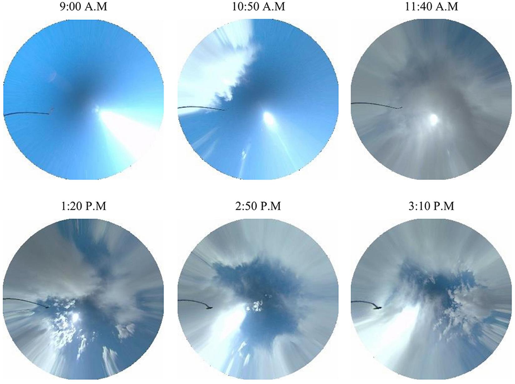
Figure 8. Cloud cover images on February 28, 2018.

The meteorological database converts these images into cloud cover coefficients between 0 and 1, which indicates the amount of cloud coverage. Figure 9 shows the results of the analytical model and the ANN for estimating the temperature of the system, along with the experimental data. According to this figure, the obtained temperature by the analytical model is lower than the actual temperature which occurs due to the absence of cloud in analytical equations. Besides, the results also show that the neural network can estimate the temperature accurately. The results of the model indicate the temperature of the radiative cooling system in the same climatic conditions but the absence of clouds in the sky. The obtained temperature difference varies up to 7°C and this diagram indicates that the cloud can affect the temperature up to 7°C. Therefore, although the radiative cooling temperature is lower than the ambient temperature despite the clouds, the absence of the cloud causes a much larger temperature difference between the system and the environment.

FIGURE 9

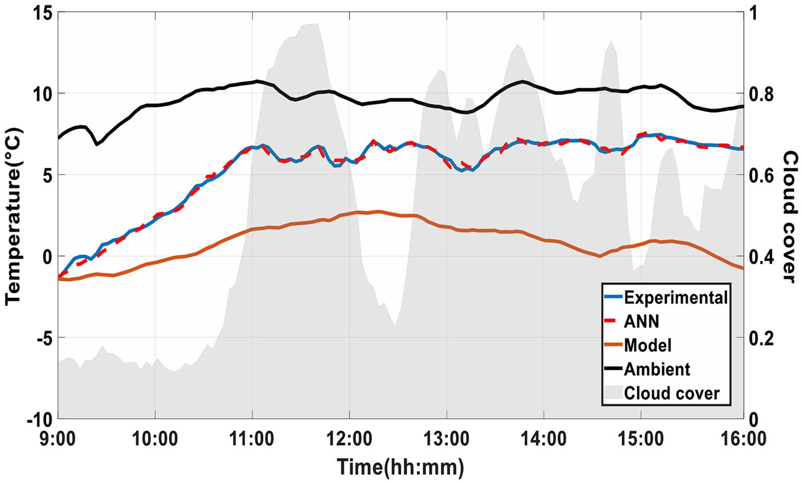
Figure 9. Model and ANN result in a cloudy day (February 28, 2018).

The artificial neural network is used to obtain the radiative cooling temperature by changing the cloud cover coefficient to predict the effect of different types of clouds on the radiative cooling temperature. Figure 10 shows the results of this study on a winter day. In this figure, the experimental temperature of the radiative cooling system is plotted as the reference data alongside the ambient temperature, with various cloud cover conditions. The predicted radiative cooling temperature is also plotted in different cloud cover coefficients obtained by the neural network. Accordingly, if β = 0 and the sky is clear during the day, the radiative cooling temperature will always be lower than the actual temperature, owing to the fact that the effect of cloud cover on the temperature of the system is usually negative. According to these figures, in the final hours, the temperature in the clear sky is the least different from the actual temperature due to the presence of small pieces of clouds during these hours. The highest difference was observed at 17:00 PM, which is equal to a 15°C temperature difference with the reference data.

FIGURE 10

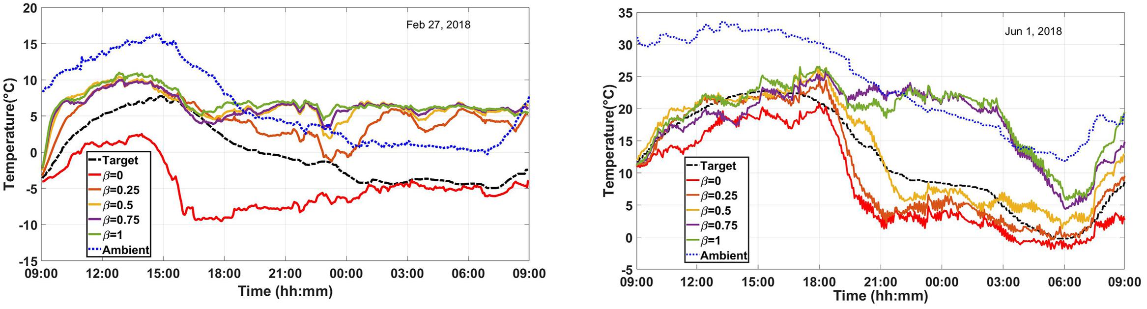
Figure 10. Predicted temperatures of radiative cooling in different cloud cover values (left) in a winter day and (right) in a summer.

Another plot is the temperature variation in the situation of 25% cloud coverage (β = 0.25). In this case, it can be observed that the temperature is higher than the reference temperature and occurs at 00:00. Afterward, the temperature of the system also rises above the ambient temperature. Similarly, the predicted temperature lines with β value of 0.5, 0.75, and 1 are drawn. In all these cases, it is realized that the system temperature rises the ambient temperature in particular hours, and the higher the cloud cover, the higher the system temperature is. Nevertheless, this relationship does not change linearly. In some hours, it is observed that the temperature of the system in low cloud cover conditions is higher than the temperature of the system in high cloud covers, which indicates the non-linear relationship between cloud cover and the net radiative cooling power of the system. In general, it can be concluded from this figure that the cloud cover can sometimes lead to an increase in the temperature of the system relative to ambient temperature.

Figure 10 also demonstrates the reference system temperature and the predicted temperature in different cloud cover conditions on a summer day. According to this figure, if the sky is cloudless, the temperature is lower than the reference mode at all times because there exist scattered clouds in the reference model. The difference varies by about 0.5°C in some hours and up to 8°C in some other hours. The system temperature for β=0.25 is higher than the temperature in a completely clear sky. Similarly, the average temperature of the system rises as the cloud cover values increases. According to this figure, it can be realized that at some certain times of the day with β=0.75, the temperature slightly higher than the temperature with β=1. This observation indicates that there is no direct relationship between cloud cover and the net radiative cooling power. Additionally, only when β is 0.75 and 1, the temperature has risen above the ambient temperature between hours of 22:00 and 04:00.

In general, from the two graphs in Figure 10, it can be concluded that the effect of cloud cover on the temperature of the radiative cooling system is unavoidable and the clear sky has the highest potential of radiative cooling power as well as the temperature reduction from the ambient. Also, these diagrams indicate that the effect of cloud cover on the system temperature of the radiator in winter is more than in summer.

Accordingly, the clouds affect the radiative cooling power, atmospheric power, and solar radiation power, and ultimately will affect the total power of the system. Considering the temperature difference between the environment and the radiative material (T_amb−T_film) as an indication for the system performance, cloud cover in the sky will affect this temperature difference. As a parameter that indicates the effect of cloud cover on the performance of the radiative cooling system, α coefficient is introduced which is calculated by Eq. 16. The α values of smaller than 1, represent a negative impact on the system and α values of greater than 1, indicate a positive impact on the system. On the other hand, if α equals 0, it means that the temperature is equal to the ambient temperature and eventually the negative values, indicate that the temperature is higher than the ambient temperature. To evaluate the effect of cloud cover on the temperature of the system and system performance using α, two winter days, and two summer days are examined in Figure 11.

FIGURE 11

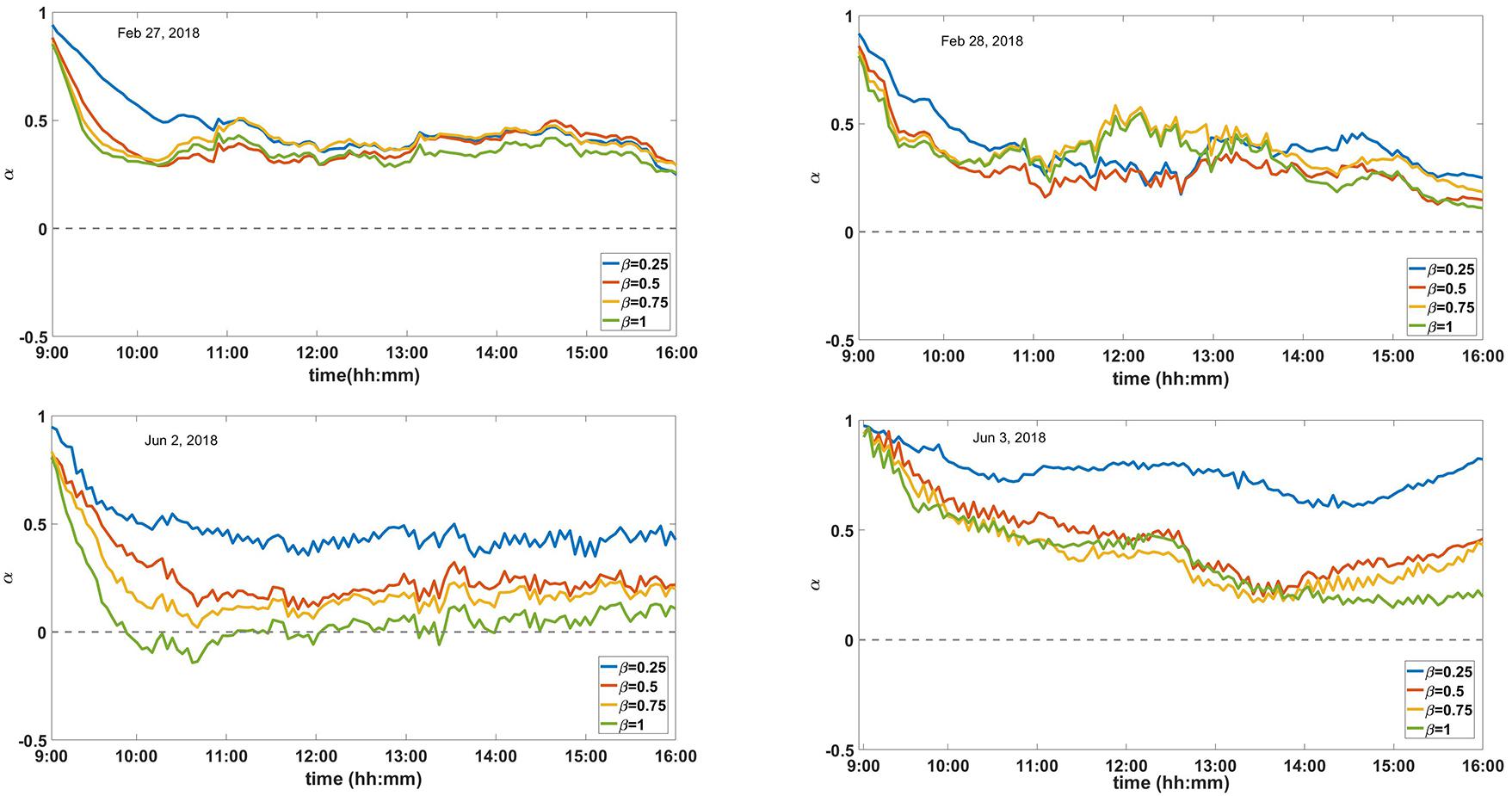
Figure 11. Impact of different cloud cover coefficients on the performance of radiative cooling on (up-left) February 27, 2018, (up-right) February 28, 2018, (down-left) June 2, 2018, and (down-right) June 3, 2018.

$$\mathrm{\alpha }=\frac{T_{amb}-T_{film,cloud}}{T_{amb}-T_{film}}(16)$$

From all these figures, it can be concluded that cloud cover never has a positive effect on the radiative cooling potential. It is also observed that in most cases, the higher the cloud coverage, the lower α, and the more negative impact it will have on the system, except as shown in Figure 11. In this figure, which is for a winter day, it is observed that less β leads to more α values comparing to the case with more cloud coveage. This is due to the complex correlation between the environmental parameters and cloud cover. Also, as can be seen from the figures, only on the second day of January 2018 a negative α in the cloudy sky conditions is observed, which means that the system temperature is higher than the ambient temperature. As an example, when β = 0.25, α is approximately equal to 0.5 and therefore, the temperature difference between the radiative film and the environment is halved.

Conclusion

Radiative sky cooling has recently been introduced as a new technology for reducing energy consumption. Various parameters affect the efficiency of a radiative cooling system such as cloud cover impact, which has been less studied in the literature. In this article, the performance of a radiative sky cooling system is precisely examined in cloudy sky conditions to understand the effect of cloud cover on the performance of the system. Due to the complexity and diversity of cloud cover and therefore the lack of a clear correlation between the cloud cover and net radiative cooling power, a recurrent artificial neural network was used to predict the function of the radiative cooling system in cloudy sky conditions. In addition to cloud cover, other environmental parameters such as ambient temperature, sunlight, wind speed, and precipitable water vapor were also considered in the development of this neural network. Besides, a mathematical model was implemented based on the temperature of the radiative cooling system in the clear sky by considering the existing analytical equations, which are valid in clear sky conditions, to compare the performance of the system is clear and cloudy sky conditions. The obtained results indicated that the existing analytical equations for radiative cooling do not take the cloud cover into account for calculating the temperature of a radiative cooling system and are only valid for clear sky conditions. Neglecting the sky cloud cover in system design can lead to temperature errors of up to 15 °C and failures in the functionality of the system. Evaluating the performance of the created neural network indicate that the temperature of the radiative cooling system can be accurately predicted by this neural network in different climatic conditions as well as in cloudy and cloudless skies. Comparison of the temperature of the system in a cloudy sky condition with different predicted cloud cover conditions demonstrated that the higher the cloud cover, the higher the system temperature and the lower the system performance would be. Nevertheless, this relationship does not change linearly. Therefore, If the cloud cover of an area is high, the radiative cooling temperature can go up to 5°C above the ambient in certain hours and the system performance can be reversed. Further studies are required to identify the impact of cloud types on the system and its measurement methods so that the behavior of the system can be predicted in cloudy conditions using analytical relationships. It is also possible to design a dual-purpose system to take advantage of the increase in the radiative cooling temperature than the ambient in cloudy skies in winter which is usually cloudy, by increasing the absorption of radiators in the atmospheric region.

Data Availability Statement

The original contributions presented in the study are included in the article, further inquiries can be directed to the corresponding author.

Author Contributions

RM implemented the code, analyzed data, performed the simulations, and plotted the figures. SF investigated, wrote the article, and organized the content. RG supervised the research and revised the first draft. All authors contributed to the article and approved the submitted version.

Conflict of Interest

The authors declare that the research was conducted in the absence of any commercial or financial relationships that could be construed as a potential conflict of interest.

References

Alnaqi, A. A., Moayedi, H., Shahsavar, A., and Khang, T. (2019). Prediction of Energetic Performance of a Building Integrated Photovoltaic/Thermal System Thorough Arti Fi Cial Neural Network and Hybrid Particle Swarm Optimization Models. Energy Conversion and Management 183, 137–148. doi: 10.1016/j.enconman.2019.01.005

CrossRef Full Text | Google Scholar

Al-waeli, A. H. A., Sopian, K., Kazem, H. A., Yousif, J. H., Chaichan, M. T., Ibrahim, A., et al. (2018). Comparison of Prediction Methods of PV/T Nano Fl Uid and Nano-PCM System Using a Measured Dataset and Arti Fi Cial Neural Network. Solar Energy 162, 378–396. doi: 10.1016/j.solener.2018.01.026

CrossRef Full Text | Google Scholar

Ammar, M. B., Chaabene, M., and Chtourou, Z. (2013). Artificial Neural Network Based Control for PV/T Panel to Track Optimum Thermal and Electrical Power. Energy Conversion and Management 65, 372–380. doi: 10.1016/j.enconman.2012.08.003

CrossRef Full Text | Google Scholar

Andreas, A., and Stoffel, T. (1981). NREL Solar Radiation Research Laboratory (SRRL): Baseline Measurement System (BMS); Golden, Colorado (Data); NREL Report No. DA-5500-56488. Golden, Colorado: NREL, doi: 10.5439/1052221

CrossRef Full Text | Google Scholar

Boriskina, S. V. (2019). An Ode to Polyethylene. MRS Energy & Sustainability 6, E14. doi: 10.1557/mre.2019.15

CrossRef Full Text | Google Scholar

Ceylan, İ, Erkaymaz, O., Gedik, E., and Etem, A. (2014). Case Studies in Thermal Engineering The Prediction of Photovoltaic Module Temperature with Artificial Neural Networks. Case Studies in Thermal Engineering 3, 11–20. doi: 10.1016/j.csite.2014.02.001

CrossRef Full Text | Google Scholar

Citakoglu, H. (2015). Comparison of Artificial Intelligence Techniques via Empirical Equations for Prediction of Solar Radiation. Computers and Electronics in Agriculture 118, 28–37. doi: 10.1016/j.compag.2015.08.020

CrossRef Full Text | Google Scholar

Crawford, T. M., and Duchon, C. E. (1999). An Improved Parameterization for Estimating Effective Atmospheric Emissivity for Use in Calculating Daytime Downwelling Longwave Radiation. Journal of Applied Meteorology 38, 474–480. doi: 10.1175/1520-04501999038<0474:AIPFEE<2.0.CO;2

CrossRef Full Text | Google Scholar

Das, A. K., and Iqbal, M. (1987). A Simplified Technique to Compute Spectral Atmospheric Radiation. Solar Energy 39, 143–155. doi: 10.1016/S0038-092X(87)80042-7

CrossRef Full Text | Google Scholar

Feng, J., Gao, K., Santamouris, M., Shah, K. W., and Ranzi, G. (2020). Dynamic Impact of Climate on the Performance of Daytime Radiative Cooling Materials. Solar Energy Materials and Solar Cells 208, 110426. doi: 10.1016/j.solmat.2020.110426

CrossRef Full Text | Google Scholar

Goldstein, E. A., Raman, A. P., and Fan, S. (2017). Sub-Ambient Non-Evaporative Fluid Cooling with the Sky. Nature Energy 2, nenergy2017143. doi: 10.1038/nenergy.2017.143

CrossRef Full Text | Google Scholar

Hu, M., Zhao, B., Li, J., Wang, Y., and Pei, G. (2017). Preliminary Thermal Analysis of a Combined Photovoltaic–Photothermic–Nocturnal Radiative Cooling System. Energy 137, 419–430. doi: 10.1016/j.energy.2017.03.075

CrossRef Full Text | Google Scholar

Huang, C., Bensoussan, A., Edesess, M., and Tsui, K. L. (2016). Improvement in Arti Fi Cial Neural Network-Based Estimation of Grid Connected Photovoltaic Power Output. Renewable Energy 97, 838–848. doi: 10.1016/j.renene.2016.06.043

CrossRef Full Text | Google Scholar

Icel, Y., Mamis, M. S., and Bugutekin, A. (2019). Photovoltaic Panel Efficiency Estimation with Artificial Neural Networks: Samples of Adiyaman, Malatya, and Sanliurfa. International Journal of Photoenergy 2019, 1–12. doi: 10.1155/2019/6289021

CrossRef Full Text | Google Scholar

Kalogirou, S. A. (2001). Artificial Neural Networks in Renewable Energy Systems Applications: A Review. Renewable and Sustainable Energy Reviews 5, 373–401. doi: 10.1016/s1364-0321(01)00006-5

CrossRef Full Text | Google Scholar

Lerch, S., and Ayari, M. L. (2020). Machine Learning for Total Cloud Cover Prediction. no. January.

Google Scholar

Lhomme, J. P., Vacher, J. J., and Rocheteau, A. (2007). Estimating Downward Long-Wave Radiation on the Andean Altiplano. Agricultural and Forest Meteorology 145, 139–148. doi: 10.1016/j.agrformet.2007.04.007

CrossRef Full Text | Google Scholar

Lu, X., Xu, P., Wang, H., Yang, T., and Hou, J. (2016). Cooling Potential and Applications Prospects of Passive Radiative Cooling in Buildings: The Current State-of-the-Art. Renewable and Sustainable Energy Reviews 65, 1079–1097. doi: 10.1016/j.rser.2016.07.058

CrossRef Full Text | Google Scholar

Martin, M., and Berdahl, P. (1984). Characteristics of Infrared Sky Radiation in the United States. Solar Energy 33, 321–336. doi: 10.1016/0038-092X(84)90162-2

CrossRef Full Text | Google Scholar

Mashaly, A. F., and Alazba, A. A. (2016). Original Papers MLP and MLR Models for Instantaneous Thermal Efficiency Prediction of Solar Still under Hyper-Arid Environment. Computers and Electronics in Agriculture 122, 146–155. doi: 10.1016/j.compag.2016.01.030

CrossRef Full Text | Google Scholar

Perveen, G., Rizwan, M., Goel, N., Anand, P., and Perveen, G. (2020). Environmental Effects Artificial Neural Network Models for Global Solar Energy and Photovoltaic Power Forecasting over India Artificial Neural Network Models for Global Solar Energy And. Energy Sources, Part A: Recovery, Utilization, and Environmental Effects 10–12. doi: 10.1080/15567036.2020.1826017

CrossRef Full Text | Google Scholar

Phys, A., Xu, S., and Tan, G. (2019). Radiative Sky Cooling: Fundamental Principles, Materials, and Applications Radiative Sky Cooling: Fundamental Principles, Materials, and Applications. Applied Physics Reviews 6, 021306. doi: 10.1063/1.5087281

CrossRef Full Text | Google Scholar

Raman, A. P., Anoma, M. A., Zhu, L., Rephaeli, E., and Fan, S. (2014). Passive Radiative Cooling below Ambient Air Temperature under Direct Sunlight. Nature 515, 540–544. doi: 10.1038/nature13883

PubMed Abstract | CrossRef Full Text | Google Scholar

Rocha, S. A. F., Guerra, F. K. O. M. V., and Guerra Vale, M. R. B. (2020). Forecasting the Performance of a Photovoltaic Solar System Installed in Other Locations Using Artificial Neural Networks. Electric Power Components and Systems 48, 1–12. doi: 10.1080/15325008.2020.1736211

CrossRef Full Text | Google Scholar

Sicart, J. E., Hock, R., Ribstein, P., and Chazarin, J. P. (2010). Sky Longwave Radiation on Tropical Andean Glaciers: Parameterization and Sensitivity to Atmospheric Variables. Journal of Glaciology 56, 854–860. doi: 10.3189/002214310794457182

CrossRef Full Text | Google Scholar

Siecker, J., Kusakana, K., and Numbi, B. P. (2017). A Review of Solar Photovoltaic Systems Cooling Technologies. Renewable and Sustainable Energy Reviews 79, 192–203. doi: 10.1016/j.rser.2017.05.053

CrossRef Full Text | Google Scholar

Siegelmann, H. T., Horne, B. G., and Giles, C. L. (1997). Computational Capabilities of Recurrent NARX Neural Networks. IEEE Transactions on Systems, Man, and Cybernetics, Part B: Cybernetics 27, 208–215. doi: 10.1109/3477.558801

PubMed Abstract | CrossRef Full Text | Google Scholar

Sivaneasan, B., Yu, C. Y., and Goh, K. P. (2017). Solar forecasting using ANN with fuzzy logic pre-processing. Energy Procedia 143, 727–732. doi: 10.1016/j.egypro.2017.12.753

CrossRef Full Text | Google Scholar

Vall, S., and Castell, A. (2017). Radiative Cooling as Low-Grade Energy Source: A Literature Review. Renewable and Sustainable Energy Reviews 77, 803–820. doi: 10.1016/j.rser.2017.04.010

CrossRef Full Text | Google Scholar

Yuan, J., Yin, H., Cao, P., Yuan, D., and Xu, S. (2020). Energy for Sustainable Development Daytime Radiative Cooling of Enclosed Water Using Spectral Selective Metamaterial Based Cooling Surfaces. Energy for Sustainable Development 57, 22–31. doi: 10.1016/j.esd.2020.04.008

CrossRef Full Text | Google Scholar

Zhai, Y., Zhai, Y., Ma, Y., David, S. N., Zhao, D., Lou, R., et al. (2017). Scalable-Manufactured Randomized Glass-Polymer Hybrid Metamaterial for Daytime Radiative Cooling. Science 355, eaai7899.

Google Scholar

Zhao, B., Hu, M., Ao, X., Chen, N., and Pei, G. (2019a). Radiative Cooling: A Review of Fundamentals, Materials, Applications, and Prospects. Applied Energy 236, 489–513. doi: 10.1016/j.apenergy.2018.12.018

CrossRef Full Text | Google Scholar

Zhao, B., Hu, M., Ao, X., Huang, X., Ren, X., and Pei, G. (2019b). Conventional Photovoltaic Panel for Nocturnal Radiative Cooling and Preliminary Performance Analysis. Energy 175, 677–686. doi: 10.1016/j.energy.2019.03.106

CrossRef Full Text | Google Scholar

Zhao, D., Aili, A., Yin, X., Tan, G., and Yang, R. (2019a). Roof-Integrated Radiative Air-Cooling System to Achieve Cooler Attic for Building Energy Saving. Energy and Buildings 203, 109453. doi: 10.1016/j.enbuild.2019.109453

CrossRef Full Text | Google Scholar

Zhao, D., Aili, A., Zhai, Y., Lu, J., Kidd, D., Tan, G., et al. (2019b). Subambient Cooling of Water: Toward Real-World Applications of Daytime Radiative Cooling. Joule 3, 111–123. doi: 10.1016/j.joule.2018.10.006

CrossRef Full Text | Google Scholar

Zuazua-Ros, A., Martín Gómez, C., Ramos, J. C., and Bermejo-Busto, J. (2017). Towards Cooling Systems Integration in Buildings: Experimental Analysis of a Heat Dissipation Panel. Renewable and Sustainable Energy Reviews 72, 73–82. doi: 10.1016/j.rser.2017.01.065

CrossRef Full Text | Google Scholar