Non-Intrusive Power Load Identification for High-Penetration Renewable Energy Grids

Introduction

In order to cope with the shortage of traditional fossil energy and increasingly severe environmental pollution, China has been vigorously developing renewable energy in recent years. The installed capacity of wind power and photovoltaic and other renewable energy has ranked first in the world, and the installed capacity has been close to 20%. The main power source of the power system will continue to increase in the future, and it is expected to exceed 50% by 2040. At the same time, due to the strong volatility and randomness of wind and solar renewable energy output, issues such as the consumption of new energy have attracted great attention from government departments, academia, and industry. More importantly, as the installed scale of renewable energy continues to expand, the operation mode and system characteristics of the traditional power grid will undergo fundamental changes, and many technical problems need to be solved urgently, especially the power load identification technology under the background of high penetration rate of new energy.

Non-intrusive power load identification (NIPLI) was first proposed by Hart in the 1980s (Tongzhi, 2012), and as one of the most important components of the advanced measurement infrastructure (AMI) (Yu, 2009), this technology is only installed as monitoring equipment at the user’s electrical entrance, records the electricity consumption data, uses the monitoring algorithm to decompose the load, and obtains the electricity consumption status and energy consumption information of the internal load. Based on NIPLI, grid companies can optimize the allocation of power resources and support the construction of smart grids (Hart, 1992). At present, non-intrusive power load identification technology is developing rapidly, and scholars have proposed a variety of load identification algorithms. L et al. (2018) designed a normal distribution measurement function that comprehensively considered the steady-state harmonic current and power characteristics, and proposed a power load identification method based on an improved chicken flock algorithm. Li et al. (2016) constructed a harmonic-based current feature expression, combined power as the objective function of device switching status identification, and used the particle swarm algorithm to search for NIPLI. L et al. (2019) proposed a load identification method based on an associative recurrent neural network model, which memorizes historical input characteristics and improves the ability to identify load characteristics. W et al. (2019) proposed an NIPLI model based on sequence-to-sequence and attention mechanisms, which improved the ability to extract and utilize load information. Tongzhi (2017); X (2018); H (2016); H et al. (2019); Y (2019) all adopted an improved or expanded HMM, which greatly improved the algorithm calculation speed and the accuracy of electrical appliance status recognition.

Unlike the traditional application scenarios of NIPLI, the high-penetration new energy grid has the characteristics of diverse load types, random power generation, and greater voltage fluctuations. The aforementioned traditional NIPLI models have their own advantages in feature extraction or load identification, but none of them considered the unknown electrical characteristics of the high-penetration new energy grid, and lacked the adaptability for power load identification in this scenario. This lack of adaptability is particularly prominent in the HMM-based NIPLI model. The observation probability and transition probability of the HMM are calculated using historical data, but past data do not guarantee that all working states of the load are measured, and all transition information of each state is determined. The aforementioned HMM-based improvements are to make full use of the existing load information but fail to take into account the changes in load characteristics and model parameter updates caused by the high-penetration new energy grid, which makes it difficult to adapt to the power load identification under the high-penetration rate of new energy grid. This article believes that the improvement ideas of non-intrusive power load identification based on the HMM under high-penetration new energy grids mainly include the following three points: 1) reduce the impact of high-penetration new energy grid environment on the determination of load status; 2) take load into account unknown observation state and new state transition, that is, the model parameters of the HMM are considered to be constantly updated to predict and calculate the implicit state of the load; and 3) the random volatility of power is considered in the power decomposition calculation.

To this end, this article proposes a non-intrusive power load identification model based on the GMM-BPHMM. The model first establishes the hidden Markov model based on load active power and current and uses the Gaussian mixture model to accurately cluster load states; after the load, implicit state sequence is encoded and the Viterbi algorithm is improved to advance its adaptability to HMM parameter updates and then to achieve optimal prediction of the load state sequence; after the load state prediction, the sequence is obtained, the random volatility of power is taken into account, and the power decomposition optimization model is established based on the principle of maximum likelihood estimation, and the calculation of power decomposition is carried out according to the mean and variance of the cluster clusters of each working state of the load, and finally verified the accuracy of the method with a calculation example.

Methods—Establishment of NIPLI

This section first proposes and establishes the NIPLI model for a new energy grid mentioned in this article and then gives a detailed description of the performance improvement of power load identification in the next section, especially in the high-penetration new energy grid.

Establishment of New Energy Power Generation System

Introduction to New Energy Management System

The household new energy management system studied in this work is mainly composed of the energy storage system, photovoltaic power generation system, fan power generation system, household appliances, and smart meters, and its structure is shown in Figure 1. The aforementioned systems realize the interconnection of information and energy between devices using power electronic converters. The smart meter collects the information of power consumption and generation every day to realize non-invasive power load identification and monitor the operation of corresponding equipment according to the demand.

FIGURE 1

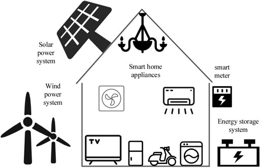
FIGURE 1. Structure chart of the household new energy management system.

Modeling of Wind Power Generation System

The power output prediction curve of the wind turbine can be obtained in advance using the wind speed prediction value in the weather forecast, and the power output value is given as follows (Marian and Fratia, 2018):

$P_{\text{vt},i}=\{\begin{array}{l}0,v<v_{\text{ci}}\hfill \\ a+bv,v_{\text{ci}}\mathrm{⩽}v<v_{\text{r}}\hfill \\ P_{\text{r}},v_{\text{r}}\mathrm{⩽}v<v_{\text{co}}\hfill \\ 0,v\mathrm{⩾}{v}_{\text{co}}\hfill \end{array},(1)$

where P_r is rated output power, v_ci is cut in wind speed, v_r is rated wind speed, v_co is cut out wind speed, constant coefficients a and b are related to wind speed and rated output power, and the calculation formula is a = P_rv_ci / (v_ci - v_r), b = - P_r / (v_ci - v_r), and units are kW and kW·s/m, respectively.

Modeling of Photovoltaic Power Generation System

The power of photovoltaic power generation is related to the ambient temperature and the actual solar radiation intensity. The specific calculation formula is as follows (Wang et al., 2016):

$P_{\text{v},i}=P_{\text{s}}{G}_{\text{a},i}\left\{k_{\text{s}}\left[T_{\text{a},i}+\frac{G_{\text{a},i}\left(T_{\text{r}}-20\right)}{800}-T_{\text{r}}\right]+1\right\}/G_{\text{s}},(2)$

where G_a and G_s are the solar radiation intensity and the light intensity under standard test (1,000 W/m²), T_r is the reference temperature of 25°C, T_a is the ambient temperature, P_v is the obtained photovoltaic power, P_s and k_s are the maximum power and power temperature coefficient under standard test, respectively, and k_s is 0.0036/°C.

Modeling of Energy Storage System

In the household energy management system, the energy storage system can store the surplus energy of renewable energy, store energy in the period of low electricity price, and supply energy for electrical equipment in the period of high electricity price so as to reduce the cost of household electricity and achieve the purpose of flexible economy. The energy storage system is composed of multiple storage batteries. The state of charge (SOC) represents the ratio of the existing capacity to the rated capacity as follows:

$SO{C}_i=\{\begin{array}{l}SO{C}_{\text{in }},i=0\hfill \\ SO{C}_{i-1}+\frac{\left(P_{\text{ESS}}^{\text{ch}}{\eta }_{\text{ch}}-\frac{P_{\text{ESS}}^{\text{deh}}}{{\eta }_{\text{dech }}}\right)\Delta i}{C_{\text{ESS}}^{\text{rated }}},1\mathrm{⩽}i\mathrm{⩽}T\hfill \end{array},(3)$

where $SO{C}_{\text{in }}$ is the initial value of the charge ratio of the energy storage battery; $C_{\text{ESS}}^{\text{rated }}$is the rated capacity; $P_{\text{ESS}}^{\text{ch}}$ and $P_{\text{ESS}}^{\text{deh}}$ are the charging power and discharge power of the energy storage system, respectively; ${\eta }_{\text{ch}}$ and ${\eta }_{\text{dech }}$represents charging efficiency and discharging efficiency, respectively; and the value in this article is 0.96. A day is divided equally into T periods, and Δi is the duration of each period (h).

Establishment of BPHMM

Introduction to HMM

The hidden Markov model is a probability model about time series (G, 2018). In the hidden Markov model, there is a time series with unobservable values and an observable time series with values determined by the aforementioned time series. Time series with unobservable values are called implicit state series, and time series with observable values are called observation series. The model structure is shown in Figure 2.

FIGURE 2

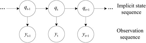
FIGURE 2. Structure chart of hidden Markov model.

An HMM can be described by the following parameters:

1) Implicit state set S:

$\text{S}=\left\{s_1,s_2,s_3,\cdots ,s_N\right\}.(4)$

2) Observation state set V:

$\text{V}=\left\{v_1,v_2,v_3,\cdots ,v_M\right\}.(5)$

3) State transition matrix:

$\mathbf{A}={\left[a_{ii}\right]}_{N\times N}.(6)$

Among them $a_{ij}=P\left(q_{t+1}=s_i\mathrm{|}{q}_t=s_i\right)$

4) Output matrix:

$\mathbf{B}={\left[b_{ik}\right]}_{N\times M}.(7)$

Among them $b_{ik}=P\left(y_t=v_k\mathrm{|}{q}_t=s_i\right)$

5) Initial probability matrix:

$\mathbf{\pi }={\left[{\pi }_i\right]}_{N\times 1}.(8)$

Among them ${\pi }_i=P\left(q_1=s_i\right)$.

It can be seen from the aforementioned formulas that the state transition probability matrix $\mathbf{A}$ and the initial state probability vector $\mathbf{\pi }$ determine the hidden state sequence, and the observation probability matrix $\mathbf{B}$ determines how to generate the observation value from the hidden state. The number N and the number M of observation states are actually defined by the previous three matrices, so the hidden Markov model can be expressed by $\lambda =\{\mathbf{A},\mathbf{B},\mathbf{\pi }\}$.

The HMM is used to study the following three types of problems:

1) Probability calculation problem. Given the model $\lambda =\{\mathbf{A},\mathbf{B},\mathbf{\pi }\}$ and the observation sequence $O=\left\{O_1{O}_2\cdots O_T\right\}$, calculate $P=\left(O\mathrm{|}\lambda \right)$.

2) Learning problems. Given the observation sequence $O=\left\{O_1{O}_2\cdots O_T\right\}$, the model parameters $\lambda =\{\mathbf{A},\mathbf{B},\mathbf{\pi }\}$ are estimated, that is, to find the maximum value $P=\left(O\mathrm{|}\lambda \right)$, the maximum likelihood estimation method is used to estimate the parameters.

3) Decoding problem. Knowing the model $\lambda =\{\mathbf{A},\mathbf{B},\mathbf{\pi }\}$ and the observation sequence $O=\left\{O_1{O}_2\cdots O_T\right\}$, the state sequence with the highest conditional probability $P=\left(I\mathrm{|}O\right)$ for a given observation sequence $I=\left\{I_1{I}_2\cdots I_{\text{T}}\right\}$ is obtained, that is, the corresponding hidden state sequence is predicted according to the given observation sequence.

Problem Modeling and Parameter Calculation

In the NIPLI study, the physical meaning of the two time series in the HMM is very clear: the implicit state sequence corresponds to the operating state of each consumer, and the observation sequence corresponds to the measurable electrical quantity. Therefore, the NIPLI problem is transformed into a problem which is to obtain the most likely hidden state sequence corresponding to the observation sequence under the given HMM parameter and observation sequence, that is, the decoding problem.

Further, this study builds the NIPLI problem into the following the HMM and calculates its parameters:

1) Implicit state set S: In the NILD problem, S can be expressed as a set of combinations of operating states of each consumer, that is, a set of total states. The set is a complete arrangement of the operating states of each consumer, and the number of elements in the set is determined by the number of clusters of the status of each consumer, and its value is calculated using the state coding method introduced in Section 3.1.3.

2) Observation state set V: In the NILD problem, V represents the collection of specific electricity information data recorded by the user’s electricity entrance. In particular, the element of the general HMM set V is the total active power, but the element in the set V of this article is a vector composed of the total active power and the total steady-state current, $v_i=\left[P_i^L,I_i^L\right]$,which is also the origin of the binary parameters in this article.

3) State transition matrix $\mathbf{A}$: $a_{ij}$ refers to the probability of transition from the total state of each consumer at time t, $q_t=s_i$, to the total state at time t + 1, $q_{t+1}=s_j$. Calculation method is given as follows:

$a_{ij}=\frac{h_{ij}}{{\displaystyle \sum _{j=1}^N{h}_{ij}}},(9)$

where $h_{ij}$ is the frequency of the total state transition from $q_t=s_i$ to $q_{t+1}=s_j$, and N is the total number of hidden states.

4) Output matrix $\mathbf{B}$:$b_{ik}$ represents the probability that each consumer is in a general state $q_t=s_i$ at time t and the observed value is $y_t=v_k$. The calculation method is given as follows:

$b_{ik}=\frac{o_{ik}}{{\displaystyle \sum _{k=1}^M{o}_{ik}}},(10)$

where $o_{ik}$ is the frequency of the total state $q_t=s_i$ at time t and the observed value is $y_t=v_k$, and M is the total number of observed values.

5) Initial probability matrix $\mathbf{\pi }$: ${\pi }_i$ represents the probability that the overall state of each consumer is $s_i$ at the initial moment. The calculation method is as follows:

${\pi }_i=\frac{d_i}{d},(11)$

where d is the total amount of data in the training set and $d_i$ represents the frequency of occurrence of hidden states$s_i$ in the training set.

It should be pointed out that the factor hidden Markov model (FHMM) can be used for the modeling of multiple appliances. The FHMM contains multiple hidden state chains, which correspond to each appliance to be studied. However, related studies have shown that the state recognition accuracy of FHMM prediction is low (G, 2018). Therefore, this article improves on the basis of the classic HMM, cooperates with the state coding method described in Section 3.1.3 to convert the combined vector of each consumer’s state into a binary value, and solves the problem that the hidden state of the HMM is difficult to be represented by a vector, while not making each consumer state compared with the FHMM, the state transition matrix decoupling theoretically retains the correlation information between the state transitions of different appliances.

Methods—Improvement of GMM-BPHMM for High-penetration New Energy Grids

Clustering and Encoding of Load Status Based on GMM

The selection of load characteristics determines the physical description of the load state, and clustering is the method of determining the load state. The selection of load characteristics and clustering methods is the first step of the method described in this article.

Selection of Load Feature

At present, the load characteristics selected by NIPLI’s research can be roughly divided into two kinds: transient and steady states. Because the transient characteristics are generally synthetic data, they are not actually collected by the measurement device, and practicability is not strong. Therefore, this study selects the steady-state electrical quantity as the load characteristic.

The steady-state electrical quantities mainly include active power and steady-state current. Active power is an indicator of power decomposition calculation. NIPLI needs to give the decomposition value of load active power after state recognition is completed, so active power is a characteristic adopted by most NIPLI research institutes. However, the steady-state power fluctuates slightly, the steady-state current is not affected by voltage fluctuations, and the calculated load recognition accuracy is higher (Z, 2016). Therefore, this study selects active power and steady-state current as load characteristics.

State Clustering

Various types of loads have different operating states during operation due to their own electrical characteristics or working conditions. From the perspective of power load identification, electrical appliances can be divided into three types of electrical appliances: switch-state electrical appliances, limited multistate electrical appliances, and continuously variable states according to their operating status (Hart, 1992). The number of operating states of the first two types of electrical appliances can be counted. In theory, all operating states can be obtained. However, the operating state of continuously variable electrical appliances changes continuously. To continue research into limited multistate electrical appliances, a clustering algorithm is required to cluster the operating states to make them discretized.

Considering that there are noisy points in the historical data, which will interfere with the hidden laws behind the model learning data so as to adversely affect the performance of the model, this study uses the GMM algorithm to extract and cluster the electrical load characteristics. The Gaussian mixture model is based on the assumption that the sample data points obtained are all independent and identically distributed, and the distribution is formed by the linear superposition of several Gaussian kernel functions (Berges, et al., 2009; Qiu, 2015). Therefore, compared with commonly used clustering algorithms such as K-means, the number of clusters in this algorithm does not need to be determined in advance, and it has multiple models, and the division is more refined. It is suitable for multi-category division and can be applied to complex object modeling and then smoothly to approximate the density distribution of any shape (Ap et al., 1977; Yu et al., 2013).

When estimating the parameters of the GMM, the expectation–maximization algorithm is generally used, so the entire GMM clustering algorithm process is as follows:

1) Let the data to be clustered be $\left\{y_1,y_2,\mathrm{...},{\text{y}}_n\right\}$, establish a Gaussian mixture model and initialize the parameters:

$P\left(y|\theta \right)={\displaystyle \sum _{k=1}^K{\alpha }_k\varphi \left(y|{\theta }_k\right)},(12)$

where ${\alpha }_k$ is the coefficient, ${\displaystyle \sum _{k=1}^K{\alpha }_k=1}$, $\varphi \left(y\right|{\theta }_k)$ is the Gaussian distribution density, ${\theta }_k=({\mu }_k,{\sigma }_k^2)$, and

$\varphi \left(y|{\theta }_k\right)=\frac{1}{\sqrt{2\pi }{\sigma }_k}\exp \left(-\frac{{\left(y-{\mu }_k\right)}^2}{2{\sigma }_k^2}\right)(13)$

is called the k-th submodel;

2) Step E: according to the current model parameters, calculates the response of submodel k to data y_j:

${\gamma }_{jk}=\frac{{\alpha }_k\varphi \left(y|{\theta }_k\right)}{{\displaystyle \sum _{k=1}^K{\alpha }_k\varphi \left(y|{\theta }_k\right)}},(14)$

where j = 1,2…,N, k = 1,2…,K;

3) Step M: calculate the model parameters of the new iteration as follows:

${\mu }_k=\frac{{\displaystyle \sum _{j=1}^N{\gamma }_{jk}{y}_j}}{{\displaystyle \sum _{j=1}^N{\gamma }_{jk}}},k=\mathrm{1,2},\mathrm{...},K(15)$

${\sigma }_k^2=\frac{{\displaystyle \sum _{j=1}^N{\gamma }_{jk}{\left(y_j-{\mu }_k\right)}^2}}{{\displaystyle \sum _{j=1}^N{\gamma }_{jk}}},k=\mathrm{1,2},\mathrm{...},K(16)$

${\alpha }_k=\frac{{\displaystyle \sum _{j=1}^N{\gamma }_{jk}}}{N},k=\mathrm{1,2},\mathrm{...},K.(17)$

4) Repeat steps (2) and (3) until convergence.

State Encoding

In most studies, vectors are generally used to represent the current state of several electrical appliances at a time (hereinafter referred to as the total state for convenience). For example, assuming that the number of states of the three electrical appliances is 2, 3, and 8, respectively, and the state at that time is, respectively, is 0, 2, and 6, and then the total state can be expressed by the vector S = [0,2,6]. However, in HMM applications, the hidden state cannot be represented by a vector. To this end, this study proposes a binary-based state coding method, which encodes the hidden state vectors of multiple appliances into a binary state value. With the previous example, the specific steps are as follows:

1) Allocate digits: Determine the binary digits required for coding according to the number of electrical appliances. The number of states of the above three electrical appliances is 2, 3, and 8, respectively, and the binary digits allocated to each electrical appliance are 1, 2, and 3, respectively.

2) Determine the value. The binary status value is calculated according to the decimal status value of the electrical appliance at the current moment. The current three electrical appliances have decimal status values of 0, 2, and 6, respectively, and the binary status values are 0, 10, and 110, respectively.

3) Splicing representation. The obtained binary state values are spliced from high to low according to the sorting of electrical appliances, and the final result is obtained. The state value of the state vector after splicing at the current time is 010110.

Table 1 shows other examples of the encoding method.

TABLE 1

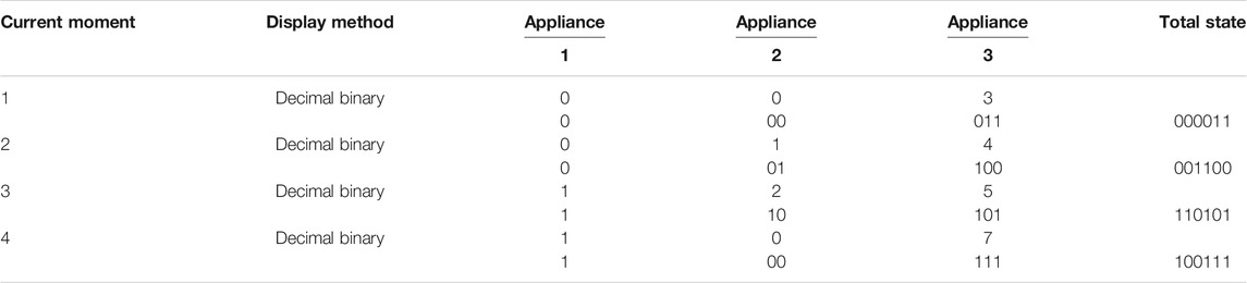
TABLE 1. State code of some electrical appliances.

Implied State Prediction Taken Into Account the Unknown Observation State and the Transition of New State

The Viterbi algorithm was proposed by the American Italian scientist Andrew Viterbi in 1967. The Viterbi algorithm is a dynamic programming algorithm used to solve the shortest path problem and is widely used in decoding and natural language processing (Forney, 1973).

The basic idea of the Viterbi algorithm is to start at t = 1 and recursively calculate the maximum probability of transitioning to each state i at time t:

$\delta \left[t,i\right]={\max }_j\left(\mathbf{B}\left[i,y_t\right]\cdot \delta \left[t-1,j\right]\cdot \mathbf{A}\left[j,i\right]\right)(18)$

And record the state from time t-1 to the state with the highest probability of state i at time t:

$\psi \left[t,i\right]={\mathrm{argmax}}_i\left(\delta \left[t-1,j\right]\cdot \mathbf{A}\left[j,i\right]\right)(19)$

After calculating the time T, find out the state ${\max }_i\left(\delta [T,i]\right)$ which the probability belongs is the end point of the prediction sequence $q_T^{\ast }$. From this point, based on the prediction, point $\psi$ is gradually obtained from back to front to obtain the optimal prediction sequence $Q^{\ast }=\left(q_1^{\ast }{q}_2^{\ast },\cdots ,q_T^{\ast }\right)$.

In the aforementioned classic Viterbi algorithm, the determination of HMM parameters is the prerequisite for the realization of the algorithm. However, in the scenario of a new energy grid with a high penetration rate, historical data cannot reflect the transfer relationship between all working states and states of the load, and the new measured data are not completely consistent with the measured electrical data. In other words, the model parameters of the HMM are not completely determined. Under this premise, the classical Viterbi algorithm that does not have the ability to adapt to unknown data is difficult to accurately solve the prediction problem of the optimal implicit sequence.

Based on the above ideas, this study proposes an improved Viterbi algorithm and makes the following improvements: 1) Considering that a new observation state will appear in electrical appliances and the observation state may correspond to the unknown operating state, this article uses the K-means algorithm to cluster into known measurement states for the new electrical data input; 2) considering that there may be new state transitions in electrical appliances, the calculation methods of $\delta$ and $\psi$ are changed based on maximum likelihood estimation; 3) considering the sparsity of the state transition matrix and measurement matrix, for example, the sparse Viterbi algorithm proposed by (Makonin et al., 2016a), the algorithm only calculates the state transition probability and the measurement probability that are not zero.

For a given observation sequence $Y=\left\{y_0{y}_1,\cdots ,y_T\right\}$ and implicit state sequence $Q=\left\{q_0{q}_1,\cdots ,q_T\right\}$, the specific steps of the improved Viterbi algorithm proposed in this article are as follows:

1) Initialization:

$\delta \left[0,i\right]=\pi \left[i\right]\cdot \mathbf{B}\left[i,y_0\right].(20)$

2) Recursive calculation:

$\delta \left[t,i\right]={\max }_j\left(\mathbf{B}\left[i,y_t\right]\cdot \delta \left[t-1,j\right]\cdot \mathbf{A}\left[j,i\right]\right)(21)$

$\psi \left[t,i\right]={\mathrm{argmax}}_j\left(\delta \left[t-1,j\right]\cdot \mathbf{A}\left[j,i\right]\right).(22)$

In particular, let us set $y_t=k$ as the measurement state at time t. When this observation state occurs, according to the principle of maximum likelihood estimation, the hidden state with the greatest probability of occurrence should be the state i that satisfies $b_{ik}=\max \left(B[:,k]\right)$.

When calculating $\delta [t,i]$ and $\psi [t,i]$, change the calculation of the above two formulas to the following:

$\delta \left[t,i\right]={\max }_j\left(\mathbf{B}\left[i,k\right]·\delta \left[t-1,j\right]\right)·\max \left(\mathbf{A}\left[:,:\right]\right)(23)$

$\psi \left[t,i\right]={\max }_j\left(\delta \left[t-1,j\right]\right)·\max \left(\mathbf{A}\left[:,:\right]\right),(24)$

where $\mathbf{A}[:,:]$represents the element in $\mathbf{A}$.

Viterbi is a dynamic programming algorithm. It only pays attention to the optimal solution at each step. It is unnecessary to study the unknown but determined non-optimal solution. Therefore, this article only focuses on the new state transition of state i that meets $b_{ik}=\max \left(\mathbf{B}[:,k]\right)$. The reason for the transition probability valued $\max \left(\mathbf{A}[:,:]\right)$ is to prevent the path passing through this point from being abandoned by the algorithm. If the algorithm does not take other legal values, the model can still get the correct result, but it will make the value smaller, thereby reducing the probability that the optimal path goes through the point in the future.

3) Calculation of termination status:

$p_T^{\ast }={\max }_i\left(\delta \left[T,i\right]\right)(25)$

$q_T^{\ast }={\mathrm{argmax}}_i\left(\delta \left[T,i\right]\right).(26)$

4) Optimal sequence backtracking:

$q_{\text{t}}^{\ast }={\psi }_{\text{t}+1}\left(q_{t+1}^{\ast }\right),t=T-1,T-2,\cdots ,0.(27)$

The sequence obtained at this time is the predicted optimal hidden state sequence $Q^{\ast }=\left(q_1^{\ast }{q}_2^{\ast },\cdots ,q_T^{\ast }\right)$.

Power Decomposition Considering the Random Volatility of New Energy Generation

Under the new energy generation, the power of electrical appliances in a certain stable operating state fluctuates, and this fluctuation can be regarded as a random observation under a certain probability distribution (Liang et al., 2010a; Liang et al., 2010b). In this study, the normal distribution is used to describe the randomness of generation fluctuations during stable operation of the appliance, and it is used to calculate the power decomposition of the appliance.

The power decomposition calculation steps in this study are as follows: 1) According to the average value and variance of the clusters of each electrical appliance sample, establish a normal distribution probability density function for each state of each electrical appliance. 2) Establish the objective function based on maximum likelihood estimation, that is, to obtain the maximum value of the joint probability, and note that the sum of the power decomposition values of the electrical appliances at the same time should be equal to the constraint condition of the total power. The power decomposition calculation model is constructed as follows:

$\{\begin{array}{l}{f}_{\left[\text{i,j}\right]}\left(\text{x}\right)=\frac{1}{\sqrt{2\pi }{\sigma }_{\left[\text{i,j}\right]}}\exp \left(-\frac{{\left(x-{\mu }_{\left[\text{i,j}\right]}\right)}^2}{2{\sigma }_{\left[\text{i,j}\right]}^2}\right)\\ \underset{P^{\left(1\right)},\dots ,P^N}{\text{max}}{\displaystyle \prod _{i=1}^N{f}_{\left[\text{i,j}\right]}\left(P^{\left(i\right)}\right)}\\ \text{s}\text{.t}.{\displaystyle \sum _{i=1}^N{P}^i=P^L}\end{array}(28)$

In the formula, ${\sigma }_{[i,j]}$ and ${\mu }_{[i,j]}$refer to the standard deviation and mean value of the j-th cluster of the i-th appliance, respectively; N is the number of appliances; $P^{\left(i\right)}$ refers to the decomposed active power of each appliance; and $P^L$ refers to the active power of the total load. $f_{[i,j]}\left(P^{\left(i\right)}\right)$ refers to the probability of $P^{\left(i\right)}$ when appliance i is in the j operating state. The a forementioned problem is a common convex quadratic programming problem after taking ln() on both sides of the objective function. The complete flow of the non-intrusive power load identification method proposed for high-penetration new energy grids in this study is shown in Figure 3.

FIGURE 3

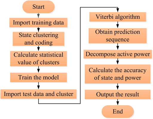
FIGURE 3. Flow chart of NIPLI based on GMM-BPHMM.

Results and Discussion

Experimental Method

Since there is no public data set containing new energy power generation equipment at present, the author will generate simulation data based on the power generation model described in Section 2.1 on the basis of the public data set, for example, analysis.

This study selects the public data set AMPds2 established by a Canadian scholar Stephen Makonin and others to verify the method described in this article (Makonin et al., 2016b). AMPds2 collects real electrical data of electrical equipment in a household and records 11 electrical characteristics, including steady-state current and active power. The sampling frequency is 1/60 Hz, and the recording time is 2 yr. It is suitable as a data set for analysis.

From the data set, select six kinds of appliances, such as fireplace (WOE), clothes dryer (CDE), dishwasher (DWE), television (TVE), washing machine (CWE), and heat pump (HPE), for a total of 14,400 sampling points in 10 days The active power and steady-state current data are divided into 10 groups according to time, which are recorded as test1-test10, and 10-fold cross-validation is performed. In each experiment, nine groups of data are selected as training data, and one group is used as test data. Finally, the average is the result. The PC configuration used in this article is 16 GB RAM/Inter (R) Core (TM) i5-8300H@2.30 GHz, written in Python.

Decomposition Result

In this study, the basic accuracy rate $AC{C}_{\text{state }}$is used to evaluate the accuracy of load state recognition, and the root-mean-square error$AC{C}_{\text{power }}$is used to evaluate the accuracy of load power decomposition as follows:

$AC{C}_{\text{state }}=\frac{{\displaystyle \sum _{t=1}^{T}I}\left(s_t=s_t^{\ast }\right)}{T}(29)$

$AC{C}_{\text{power }}=\sqrt{\frac{1}{ \text{T}}{\displaystyle \sum _{\text{t}=1}^T{\left(p_t-p_t^{\ast }\right)}^2}}.(30)$

In the formula, T is the length of the sampling period; $s_t$and $p_t$are the actual state and actual power value of the appliance at time t, respectively; $s_t^{\ast }$and $p_t^{\ast }$are the predicted state and decomposition power value, respectively; and I () is the indicator function.

Select the superposition value of active power of six electrical appliances on a certain day as the test set. The decomposition results are shown in Figures 4–9, respectively. The yellow line is the actual power, and the green line is the decomposition result.

FIGURE 4

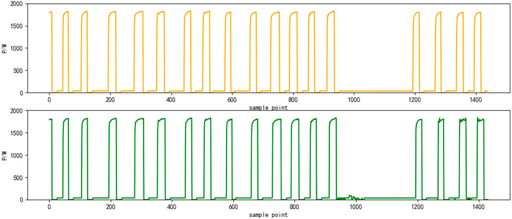
FIGURE 4. Results of power decomposition (HPE).

FIGURE 5

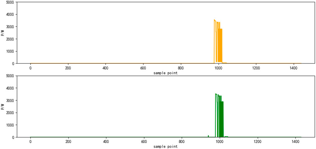
FIGURE 5. Results of power decomposition (WOE).

FIGURE 6

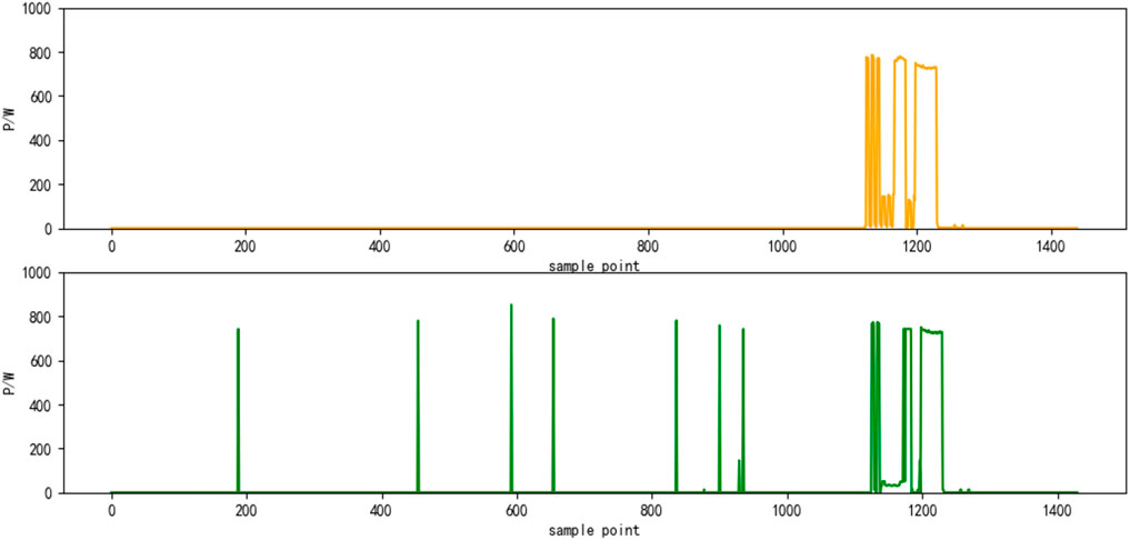
FIGURE 6. Results of power decomposition (CDE).

FIGURE 7

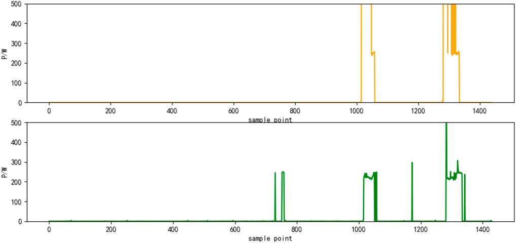
FIGURE 7. Results of power decomposition (CWE).

FIGURE 8

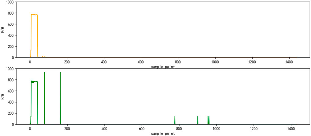
FIGURE 8. Results of power decomposition (DWE).

FIGURE 9

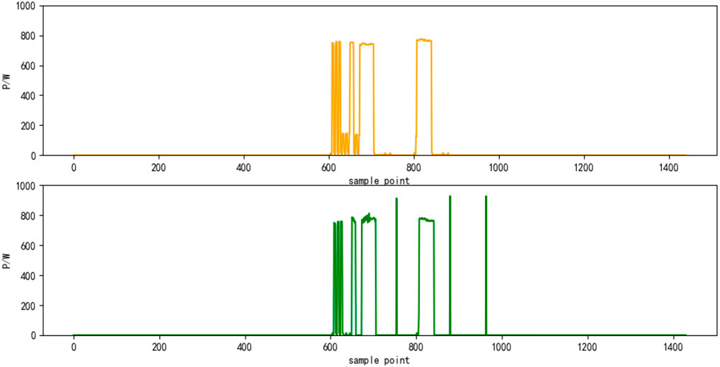
FIGURE 9. Results of power decomposition (TVE).

This study selects the decomposition method based on the genetic algorithm (GA) proposed in Q et al. (2018), the decomposition method based on deep sequence translation model in W and G (2020) and the classic HMM (G, 2018) as comparison, and uses the same data to perform the 10-fold cross-validation calculation The average value, the average accuracy rate of load state identification by the four methods, and the average accuracy rate of power decomposition are shown in Table 2 and Figure 10, respectively. It can be seen that the load decomposition method based on the binary parameter HMM and the sparse Viterbi algorithm has a better effect on the state identification and power decomposition of the total load.

TABLE 2

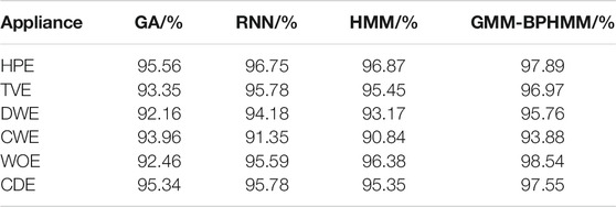
TABLE 2. Comparison of average accuracy of state recognition.

FIGURE 10

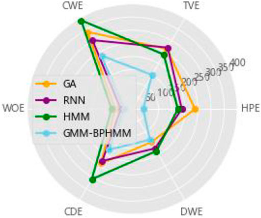
FIGURE 10. Comparison of average accuracy of power decomposition.

It can be seen from the aforementioned results that compared with the classic HMM algorithm, the use of the combined electrical characteristics of the method described in this article can enable the model to extract the operating state that better reflects the characteristics of the load, thereby improving the solution of the NIPLI problem in the high-permeability new energy grid performance. The power decomposition optimization model proposed in this study based on maximum likelihood estimation considers and learns the volatility behind the new energy generation to a certain extent, ensuring that the sum of the monitored power of each electrical appliance is equal to the total load power, making the power decomposition more accurate. For the more cutting-edge deep learning methods, the method described in this article is better than the deep learning–based solution in the accuracy of state recognition of multiple working state appliances, such as TVs and washing machines.

Conclusion

This article proposes non-intrusive power load identification under high-penetration new energy grids. This method proposes and constructs the binary parameter hidden Markov model BPHMM, uses the GMM algorithm to cluster the load characteristics, proposes a binary-based coding scheme to encode the load state combination, and improves the Viterbi algorithm to make it have the adaptability of the updating model parameter situation and then realize the optimal prediction of the load state. Finally, an optimization model that takes into account the random volatility of the new energy generation is established, and the power decomposition of the load is realized according to the mean and variance of the appliance cluster. The results of the calculation example show that in the high penetration rate new energy grid scenario, compared with the recognition scheme based on heuristic algorithms, deep learning methods, and classic HMM, the method proposed in this article has achieved higher load status recognition accuracy and lower power decomposition error. This article proposes various measures to improve the performance of the NIPLI model under high-penetration new energy grids, such as denoising data, improving traditional methods to increase its adaptability to unknown data, and enabling the model to learn the statistical characteristics behind data fluctuations. And other ideas, I also believe that it has reference value for the practicality of NIPLI.

The research on the high-penetration new energy grid in this work is still relatively preliminary, and the non-electrical characteristics of load operation are not considered. The next step of research will focus on how to use non-electrical characteristics, such as load working hours and user behavior habits, study the processing of new unknown electrical appliances, and propose a more practical non-intrusive power load identification method.

Data Availability Statement

The original contributions presented in the study are included in the article/supplementary material; further inquiries can be directed to the corresponding author.

Author Contributions

BL contributed to conceptualization, methodology. ZT contributed to project administration, funding acquisition, and formal analysis. XS contributed to data curation, visualization, and writing. All authors contributed to the article and approved the submitted version.

Funding

The paper is supported by Science and technology project of China Southern Power Grid Co., Ltd (Grant No. 066600KK52180051).

Conflict of Interest

BL and ZT were employed by the company Electric Power Research Institute of Guizhou Power Grid Co., Ltd. XS was employed by the company Suzhou Huatian Power Technology Co., Ltd.

References

Ap, D., Laird, N. M., and Rubin, D. B. (1977). Maximum Likelihood From Incomplete Data Via the EMAlgorithm. J. R. Stat. Soc. Ser. B (Methodological) 39 (1), 1–22. doi:10.1111/j.2517-6161.1977.tb01600.x

CrossRef Full Text | Google Scholar

Berges, M., Goldman, E., Matthews, H. S., and Soibelman, L. (2009). Learning Systems for Electric Consumption of Buildings [M], 1–10.

Forney, G. D. (1973). The Viterbi Algorithm. Proc. IEEE 61 (3), 268–278. doi:10.1109/proc.1973.9030

CrossRef Full Text | Google Scholar

G, D. (2018). Study on Non-intrusive Load Decomposition of Residential Electricity Based on HMM [D]. Beijing: North China Electric Power University.

H, A. J., Yong-Sheng, W., Bo-Chuan, G. U., Xiao-Feng, L., and Yi, S. (2019). Non-intrusive Load Monitoring Method Based on Denoising Filtering and FHMM. Automation & Instrumentation 34 (11), 97–102. doi:10.19557/j.cnki.1001-9944.2019.11.023

Google Scholar

H, C. (2016). Study on Nonintrusive Load Monitoring Technology Based on HMM and its Variants[D]. Tianjin: Tianjin University.

Hart, G. W. (1992). Nonintrusive Appliance Load Monitoring. Proc. IEEE 80 (12), 1870–1891. doi:10.1109/5.192069

CrossRef Full Text | Google Scholar

L, H., Shuaibin, S., Xuhui, X. U., Dongguo, Z., Ruolin, M., and Wensha, H. (2019). A Non-intrusive Load Identification Method Based on RNN Model. Power Syst. Prot. Control. 47 (13), 162–170. doi:10.19783/j.cnki.pspc.180785

Google Scholar

L, X., Meihan, C., and Yuejuan, X. U. (2018). Non-intrusive Load Monitoring Based on Improved Chicken Swarm Optimization Algorithm. Electric Power Automation Equipment 38 (5), 235–240. doi:10.16081/j.issn.1006-6047.2018.05.033

Google Scholar

Li, R., Mingshan, H., Dongguo, Z., Hong, Z., and Wenshan, H. (2016). Optimized Nonintrusive Load Decomposition Method Using Particle Swarm Optimization Algorithm. Power Syst. Prot. Control. 44 (8), 30–36. doi:10.7667/PSPC160239

Google Scholar

Liang, J., Ng, S. K. K., Kendall, G., and Cheng, J. W. M. (2010a). Load Signature Study—Part I: Basic Concept, Structure and Methodology. IEEE Trans. Power Deliv. 25 (2; 2), 551–560. doi:10.1109/TPWRD.2009.2033799

Liang, J., Ng, S. K. K., Kendall, G., and Cheng, J. W. M. (2010b). Load Signature Study-Part II: Disaggregation Framework, Simulation, and Applications. IEEE Trans. Power Deliv. 25 (2), 561–569. doi:10.1109/tpwrd.2009.2033800

CrossRef Full Text | Google Scholar

Makonin, S., Ellert, B., Bajić, I. V., and Popowich, F. (2016b). Electricity, Water, and Natural Gas Consumption of a Residential House in Canada from 2012 to 2014. Sci. Data 3 (1), 160037. doi:10.1038/sdata.2016.37

PubMed Abstract | CrossRef Full Text | Google Scholar

Makonin, S., Popowich, F., Bajic, I. V., Gill, B., and Bartram, L. (2016a). Exploiting HMM Sparsity to Perform Online Real-Time Nonintrusive Load Monitoring. IEEE Trans. Smart Grid 7 (6), 2575–2585. doi:10.1109/tsg.2015.2494592

CrossRef Full Text | Google Scholar

Marian, M., and Fratia, M. (2018). Photogrammetric Measurement of a Wooden Truss. Slovak J. Civil Eng. 26 (4), 1–10. doi:10.2478/sjce-2018-0022

CrossRef Full Text | Google Scholar

Q, X., Lou, O., Zheng, A., and Liu, Y. (2018). A Non-intrusive Load Decomposition Method Based on Affinity Propagation and Genetic Algorithm Optimization. Trans. China Electrotechnical Soc. 33 (16), 3868–3878. doi:10.19595/j.cnki.1000-6753.tces.170894

CrossRef Full Text | Google Scholar

Qiu, T. (2015). EM Algorithm Based on Gaussian Mixture Model and its Application [D]. Chengdu: University of Electronic Science and Technology.

Tongzhi, L. (2017). Research on Event-Based HMM for Non-intrusive Electrical Load Monitoring Algorithm [D]. Wuhan: Huazhong University of Science and Technology.

Tongzhi, L. (2012). Technical Implications and Development Trends of Flexible and Interactive Utilization of Intelligent Power. Automation Electric Power Syst. 36 (2), 11–17.

Google Scholar

W, K., Haiwang, Z., Nanpeng, Y. U., and Qing, X. (2019). Nonintrusive Load Monitoring Based on Sequence-To-Sequence Model with Attention Mechanism. Proc. CSEE 39 (1), 75–83. doi:10.13334/j.0258-8013.pcsee.181123

Google Scholar

W, R., and G, X. (2020). Non-intrusive Load Decomposition Method Based on Deep Sequence Translation Model. Power Syst. Tech. 44 (01), 27–37. doi:10.13335/j.1000-3673.pst.2019.0645

Google Scholar

Wang, J., Wei, K., Zhang, J., Lin, T., and Bao, X. (2016). “Measurement Method for Vertical Tank Deformation Based on Laser Scanning Principle,” in 2016 3rd International Conference on Systems and Informatics (ICSAI). (New York, NY: IEEE), 583–587.

Google Scholar

X, S. (2018). Research on Non-intrusive Load Decomposition Based on FHMM [D]. Zhengzhou: Zhengzhou University.

Y, W. (2019). Non-intrusive Load Decomposition Method Based on Factorial Hidden Markov Model [D]. Beijing: North China Electric Power University.

Yu, Y., Bo, L., and Wenpeng, L. (2013). Nonintrusive Residential Load Monitoring and Decomposition Technology. South. Power Syst. Tech. 7 (4), 1–5. doi:10.13648/j.cnki.issn1674-0629.2013.04.004

Google Scholar

Yu, Y. X. (2009). Technical Composition of Smart Grid and its Implementation Sequence. South. Power Syst. Tech. 3 (2), 1–5. doi:10.13648/j.cnki.issn1674-0629.2009.02.020

Google Scholar