Forecasting Electricity Load With Hybrid Scalable Model Based on Stacked Non Linear Residual Approach

Power has totally different attributes than other material commodities as electrical energy stockpiling is a costly phenomenon. Since it should be generated when demanded, it is necessary to forecast its demand accurately and efficiently. As electrical load data is represented through time series pattern having linear and non-linear characteristics, it needs a model that may handle this behavior well in advance. This paper presents a scalable and hybrid approach for forecasting the power load based on Vector Auto Regression (VAR) and hybrid deep learning techniques like Long Short Term Memory (LSTM) and Convolutional Neural Network (CNN). CNN and LSTM models are well known for handling time series data. The VAR model separates the linear pattern in time series data, and CNN-LSTM is utilized to model non-linear patterns in data. CNN-LSTM works as CNN can extract complex features from electricity data, and LSTM can model temporal information in data. This approach can derive temporal and spatial features of electricity data. The experiment established that the proposed VAR-CNN-LSTM(VACL) hybrid approach forecasts better than more recent deep learning methods like Multilayer Perceptron (MLP), CNN, LSTM, MV-KWNN, MV-ANN, Hybrid CNN-LSTM and statistical techniques like VAR, and Auto Regressive Integrated Moving Average (ARIMAX). Performance metrics such as Mean Square Error, Root Mean Square Error, and Mean Absolute Error have been used to evaluate the performance of the discussed approaches. Finally, the efficacy of the proposed model is established through comparative studies with state-of-the-art models on Household Power Consumption Dataset (UCI machine learning repository) and Ontario Electricity Demand dataset (Canada).

1 Introduction

As an option of petroleum products to create power, elective asset like sunlight based, wind and so on have become , quite possibly, the most encouraging sustainable power sources within the presence of greenhouse effect and polluted environment (Miller et al., 2009). The electric grid framework is complex since it should keep up the equilibrium among production, transmission and distribution of power. Taking into account the yield power from an alternate source is trademark in instability and discontinuity, presenting incredible difficulties to load dispatching, exact electrical load estimating assumes a significant part in soothing the pressing factor of managing top load and improving robustness limit with respect to electrical load demand. Electricity demand forecasting plays an important role as it enables the electric industry to make informed decisions in planning power system demand and supply. Moreover, accurate power demand forecasting is necessary as energy must be utilized as it is produced due to its physical characteristics (Ibrahim et al., 2008). Albeit ample studies have been dedicated to building powerful models to predict accurate electrical load (Du et al., 2019), the greater part of them are utilized for producing deterministic point prediction with single-variable yield each time. Generally applied point estimating models for electrical load can be partitioned into two classes: statistical models and machine learning models. Statistical models exploit as completely as conceivable the past records by giving attention to connections and patterns between the old and future exhibition of power load data dependent on the development of mathematical models (Ma et al., 2017). Nevertheless, statistical strategies can diminish the anticipating mistakes when the data features are under ordinary conditions, having high prerequisite for simple time series. Work like ARMA (Bikcora et al., 2018) and ARIMA (Wu et al., 2020) address traditional time series prediction strategies, however they ordinarily neglect to consider the impact of other covariate factors (Wu et al., 2020). Therefore, to counter the weaknesses of statistical models, machine learning models, known as artificial neural networks (ANN), are deployed for power load forecasting (Khwaja et al., 2020), (Wu et al., 2019) and (Xiao et al., 2016).

As a promising part of AI strategies, deep learning, mostly referring to multi-layer network having feature learning potential, has acquired a wide recognition for power load prediction due to three significant properties: solid generalization ability, large scale data processing and unsupervised way for the feature learning. From the work (Bedi and Toshniwal, 2019), it is widely perceived that deep learning models exhibit good performance in terms of precision, scalability and stability. Nonetheless, one of significant criticisms of picking up deep learning algorithms is, it lacks strong theoretical foundation and mathematical induction. This is additionally an effectively a disregarded issue in the viable use of electrical load prediction. To keep away from that issue, this paper presents a mathematical form of problem formulation followed by the proposed solution as VACL model which is a combination of statistical model VAR and Deep Learning methods CNN,LSTM. The present work is an extension of our previous work (Sinha et al., 2021).

Electricity demand forecasting can be of multiple types: short term (day), medium term (week to month) and long term (year). These forecasts are necessary for the proper operation of electric utilities. Precise power load forecasting can be helpful in financing planning to make a strategy of power supply, management of electricity, and market search (Stoll and Garver, 1989). It is a time series problem that is multivariate as electrical energy depends on many characteristics that use temporal data for the prediction. Temporal data depends on time and represented using time stamps. Prediction using classical load forecasting methods is challenging as power consumption can have a uniform seasonal pattern but an irregular trend component. To continue the discussions, the rest of the paper is organized as: Section 2,literature review of existing state-of-the-art models and issues relatingto them that will lead to the problem statement as presented in Section 3. To understand the basics about the multivariate time series analysis and deep learning forecasting strategies, section 4 is presented. In continuation to existing approach, Section 5 presents the detail about proposed methodology followed by Section 6 which consists of experimental studies and discussion of application of proposed model on two large datasets. Finally,Section 7 is about conclusion and states the future scope of the proposed method.

2 Literature Review

The new improvement of deep learning models, like Deep Neural Network (DNN), Recurrent Neural Network (RNN), Convolutional Neural Network (CNN), has had an incredible impact in the fields of Natural Language Processing (NLP), computer vision, and recognition of speech. DNN can exhibit to model a function which is complex in nature and can efficiently mine important features of a dataset. Many researchers have explored these techniques for the multivariate time-series forecasting. Some of the recent advancement in this area is summarized as:

Authors in (Choi, 2018) discussed the ARIMA-LSTM hybrid model for time series forecasting. They used LSTM for temporal dependencies and their long-term predictive properties. To circumscribe linear properties, ARIMA is used, and for residuals that contain non-linear and temporal properties, LSTM is used. This hybrid model is compared with other methods, and it gave better results for evaluation metrics such as Mean Squared Error (MSE), Root Mean Squared Error (RMSE), and Mean Absolute Error (MAE). In (Kim and Cho, 2019), authors proposed a hybrid CNN-LSTM model that is evaluated on power consumption data. It is proposed that CNN can extract temporal and spatial features between several variables of data. In contrast, LSTM takes data returned by CNN as input and models temporal data and irregular trends. The proposed model is compared with other models like GRU, Bi-LSTM, etc., and it performed better on evaluation metrics such as MSE, RMSE, MAE, MAPE, etc. While Mahalakshmi et al. surveyed various methods for forecasting time series data and also discussed various types of time-series data that are being forecasted (Mahalakshmi et al., 2016), research has been done on various types of data such as electricity data, stock market data, etc. The performance evaluation parameter such as MAE, MSE proves that the hybrid forecasting model yields good results compared to other models. To investigate the forecasting outcome for non-linear data, Gasperin et al. discussed the problem of accurately predicting power load forecast owing to its non-linear nature (Gasparin et al., 2019). The authors worked on two power load forecast datasets and applied state-of-the-art deep learning techniques to short-term prediction data. Most relevant deep learning models applied to the short-term load forecasting problem are surveyed and experimentally evaluated. The focus has been given to these three main models: Sequence to Sequence Architectures, Recurrent Neural Networks, and recently developed Temporal Convolutional Neural Networks. LSTM performed better as compared to other traditional models. In continuation to use the deep learning models for forecasting no-linear data, authors in (Erica, 2021) propose a novel short-term load forecasting approach with Deep Neural Network architecture,CNN components to learn complex feature representation from historical load series,then the LSTM based Recurrent Neural component models the variability and dynamics in historical loading.

Siami-Namini et al. in their proposed work (Siami-Namini et al., 2018) compared deep learning methods such as LSTM with the traditional statistical methods like ARIMA for financial time series dataset. According to them, a forecasting algorithm based on LSTM improves the prediction by reducing the error rate by 85% when compared to ARIMA. On the similar lines, Wang et al. (Wang et al., 2016) worked on CNN-LSTM consisting of two parts: regional CNN and for predicting the VA rating method used is LSTM. According to their evaluation, regional CNN-LSTM outperformed regression and traditional Neural Network-based methods. Authors in (Sherstinsky, 2018) explained the essential fundamentals of RNN and CNN. They also discussed “Vanilla LSTM” and discussed the problems faced when training the standard RNN and solved that by RNN to “Vanilla LSTM” transformation through a series of logical arguments. The work done in (Hartmann et al., 2017) adopted the Cross-Sectional Forecasting approach on the AutoRegression model. It consumes available data from multiple same domain time series in a single model, covering a wide domain of data that also compensates missing values and quickly calculates accurate forecast results. This model can only deal with linear data but with multiple time series simultaneously while in (Choi and Lee, 2018), authors presented a novel LSTM ensemble forecasting algorithm that can combine many forecast results from a set of individual LSTM networks. The novel method can capture non-linear statistical properties and is easy to implement and is computationally efficient. In another domain with similar characteristics, Chniti et al. (Chniti et al., 2017) presented robust forecasting methods for phone price prediction using Support Vector Regression (SVR) and LSTM. Models have been compared for both univariate and multivariate data. In the multivariate model, LSTM performed better as compared to others. Another work like (Yan et al., 2018) attempted short-term load forecasting (STLF) for the electric power consumption dataset. Due to the varying nature of data for electricity, traditional algorithms performed poorly as compared to LSTM. To increase further accuracy, the authors discussed a hybrid approach consisting of CNN on top of LSTM and experimented on five different datasets. It performed fairly better than ARIMA, SVR, and LSTM alone. As a more advanced hybrid model, authors in (Babu and Reddy, 2014) proposed a linear and non-linear models combination that is a combination of ARIMA and ANN models where ARIMA is used for linear component and ANN for a non-linear component. For further improvement, the authors proposed that the nature of time series should be taken into account so volatile nature is taken into account by moving average filter, and then hybrid model applied; the proposed hybrid model is compared with these individual models and some other models, and it performed fairly well as compared to other models. While the work in (Shirzadi et al., 2021) showed that by utilizing deep learning, the model could foresee the load request more precisely than SVM and Random Forest (RF). However, it does not validate the result on more than one dataset. In (Bendaoud and Farah, 2020) another type of CNNN for one-day ahead load estimate utilizing a two-dimensional information layer (remembering the past states’ utilizations for one layer and climatic and relevant contributions to another layer). They applied their model to a contextual analysis in Algeria and announced MAPE and RMSE of 3.16 and 270.60 (MW), individually. An approach based on clustering techniques, authors in (Talavera-Llames et al., 2019) introduced a clustering technique dependent on kNN to predict power price utilizing a multivariate dataset. The proposed model was applied on a power dataset in Spain (OMIE-Dataset, 2020) and the authors juxtaposed the outcome with existing state of art methods like MV-ANN (Hippert et al., 2001), MV-RF and traditional multivariate Box-Jenkins (Lütkepohl, 2013) model like ARIMAX (Box et al., 2011), autoregressive-moving-average (ARMAX) and autoregressive (ARX).

Coming to a more popular model, authors have proposed Elmann Recurrent Neural Networks (ERNN) in Elman (1990) to sum up feedforward neural network to better take care of ordered sequential data like time-series. Notwithstanding of the model simplicity, Elmann RNNs are difficult to prepare because of less efficiency of gradient (back) propagation. While forecasting the time series with Multi-Step Prediction method, authors in Sorjamaa and Lendasse (2006) proposed a DirRec strategy based on the combination of Recursive and Direct strategy. In this approach, a model is trained in a single mode to predict one next step of the time series data and combine it with a multiple model predictor with the same input. Authors in Bontempi (2008) presented a model as MIMO strategy where a single model is evolved to predict complete output sequence in a single effort. However the more advanced popular model known as DIRMO model Taieb et al. (2009) was proposed which is like a tradeoff with the MIMO and Direct approach. This model was proved to be more advanced in terms of multistep forecasting and computational time.

In a nut shell, the above literature survey generally centers around DNN, RNN and CNN models and shows that deep learning strategies can convey much better load forecasting precision than those accomplished by traditional models. Other deep learning models have not been investigated much for load forecastings, for example, attention model (Bourdeau et al., 2019), ConvLSTM and BiLSTM. Notwithstanding the works referred to, a different researchers have also centered around load anticipating at the structure scale, utilizing AI and deep learning strategies (Rashid et al., 2009), (Shi et al., 2017) and (Rahman et al., 2018). In any case, fewer investigations have analyzed the capacity of information digging methods for large-scale data and established their model’s efficacy on multiple datasets with different characteristics.

3 Load Forecasting Intricacies

Stemming out the research gap from the literature survey from Section 2, the present work aims at building a model that can accurately forecast power load data. The mathematical formulation and objectives of the problem is as follows:

1) Given fully observed time series data Y = {y₁, y₂,., y_T} where y_t belongs to Rⁿ and n is the variable dimension, aim is to predict a series of future time series data

2) That is, assuming {y₁, y₂,., y_T} is available, then predicting y_T+h where h is the desirable time horizon ahead of the current timestamp (Chatfield, 1996).

3) The following constraints need to be satisfied by the model:

a) Model should be able to handle numerous series data

b) Model should be able to handle incomplete data

c) Model should be able to handle noisy data

4 Multivarite Time Series Analysis With Deep Learning

4.1 Time Series

It is a series of discrete data points which are taken at fixed intervals of time (Wikipedia, 2021). An explicit order dependence is added between observations by time series via time dimension. Order of observations in time series gives a source of extra information which can be used in forecasting. There may be one or more variables in the time series. A time series that is having one variable changing over time is univariate time series. If greater than one variable varying with time, then that time series is multivariate.

It can have applications in many domains such as weather forecasting, power load forecasting, stock market prediction, signal processing, econometrics, etc.

4.2 Time Series Analysis

It constitutes methods for analyzing and drawing out meaningful information and patterns from data which can help in deciding the methods and getting better forecasting results (Cohen, 2021). It helps to apprehend the nature of the series that is needed to be predicted.

4.3 Time Series Forecasting

Time series forecasting involves creating a model and fitting it on a training set (historical data) and then using that model to make future predictions. In classical statistical handling, taking forecasts in the future is called extrapolation. A time series model can be evaluated by forecasting the future term and analyzing the performance by specific evaluation metrics like MSE, MAE, and RMSE.

4.4 Time Series Types

Time series forecasting techniques are inspired by various research on machine learning and have been changed from regression models to neural network-related models. There are multiple types of time series, of which two types are most common.

•STATIONARY: If statistical properties like mean, variance, autocorrelation, etc., of time series do not change with time, then that time series is stationary. As we know, stationary processes are easy to predict; we simply need to find out their statistical properties, which will remain the same over a while.

•NON-STATIONARY: In a non-stationary time series, data points have statistical properties like mean, variance, covariance, etc. and vary with time. There may be non-stationary behavior like trends, seasonality, and cycles that exists in the series data. Some of the most common patterns observed in non-stationary time series are(Erica, 2021):

•TREND: If there is a long duration increment or decrement in data, then trend exists. It need not be linear.

•SEASONALITY: When seasonal factors such as month of year, day of month etc. impact time series, then seasonal patterns are said to exist in time series with firm and known frequency.

•CYCLIC: When data exhibit rise and fall patterns without fixed period, then cyclic patterns occur.

4.5 Time Series Evaluation Metrics

The most commonly used error metrics for forecasting are:

• MEAN SQUARED ERROR: It is the average cumulative sum of the square of all prediction errors. It is formulated as:

$MSE=\sum _{i=1}^n{(y_i-\widehat{y}i)}^2/n(1)$

• MEAN ABSOLUTE ERROR: It is the average cumulative sum of the absolute value of all prediction errors. It is formulated as:

$MAE=\sum _{i=1}^n\Vert y_i-\widehat{y}i\Vert /n(2)$

• ROOT MEAN SQUARED ERROR: It is a square root of the mean of the cumulative sum of the square of all prediction error. It is formulated as:

$RMSE=\sqrt{\sum _{i=1}^n{(y_i-\widehat{y}i)}^2/n}(3)$

4.6 Terminology in Time Series Forecasting

• DIFFERENCING: It is a technique to transform non-stationary time series into a stationary one. In differencing, we take the difference of each value in the time series from its next value and continue until the new series become stationary.

• AIC: It refers to Akaike’s Information Criterion. For models such as VAR, it provides information about how well a model can be fitted on the data by considering the terms count in the model.

• NOISE: The randomness in data series is frequently known as noise.

• TIME SERIES MODEL: It is a derived function that considers past observations of time series along with some parameters to predict the future.

• WEIGHT: Weights stipulate the importance given to individual parameters in forecasting, respectively. In order words, it decides the impact of each item on forecasting.

• DECOMPOSITION: It refers to splitting a time series into seasonal, trend, and cyclic components.

4.7 Artificial Neural Network

Artificial Neural Network (ANN) (Yao, 1993) consists of nodes that are interconnected, simulating neurons in the biological neural system. It can be utilized for various tasks such as regression, forecasting, and pattern recognition in circumstances of complex features such as seasonality and trends observed, handling linear and non-linear data, etc. ANN model that is being used is Multilayer Perceptron, as earlier ANNs consists of only a single layer with no hidden layers, which resulted in some limitations:

• Single neurons cannot solve complex tasks.

• The model cannot learn difficulty in learning non-linear features.

MLP is a feed-forward neural network that is comprised of inputs, many hidden layers, and an output layer (Shiblee et al., 2009). In MLP, every layer is connected fully to the next layer such that neurons between contiguous layers are fully connected while neurons between the same layers have no connection. Input is fed into the input layer, and output is extracted from the output layer. The number of the hidden layers can be increased to learn more complex features according to the task.

Input represents the data that is needed to be fed in the model. Data and weights are fed to next layer. Suppose X$\left(x_1,x_2,\dots ,x_n\right)$ be the input vector and w$\left(w_1,w_2,\dots ,w_n\right)$ are weights associated for a neuron,then input to neuron of hidden layer is Input:

$f(X)=\sum _{i=1}^n(x_i.w_i)(4)$

Primary learning of the model takes place at the hidden layer (also known as the processing unit). Using the activation function, it remodels the value received from the input layer. Activation function is non-linear function applied on hidden layer input that enables the model to describe erratic relations. Sigmoid, ReLU, and tanh are the most widely used activation functions. Activation Functions mostly used are as (Yao, 1993):

• SIGMOID: It is formulated as:

$\sigma =1/(1+e^{-\mathrm{x}})(5)$

• Rectified Linear Unit (ReLU): It is most extensively used activation function having a minimum 0 threshold and formulated as:

$f(x)=max(0,x)(6)$

• tanh(x): Non-linear activation function with values lying between 0 and 1. It is formulated as:

$tanh(x)=2/(1+e^{-2\mathrm{x}})-1(7)$

The main issue with MLP is the adjustment of its weights in the hidden layer, which is necessary to get better results as output, is dependent on these weights to minimize the error. Back propagation is used for the adjustment of weight parameters in the hidden layer. After loss calculation in the forward pass, the loss is backpropagated, and the model weights are updated via gradient descent. Backpropagation rule is given mathematically as:

$\delta w=w-w_{\text{prev}}=-\eta \ast \frac{\delta E}{\delta w}(8)$

Where weights are represented by w, E(w) represents cost function, representing how far the predicted output is, from actual output, and η represents the learning rate.

4.8 Long Short Term Memory

RNN (Jordan, 1990), (Elman, 1990), (Chen and Soo, 1996) are types of neural networks where the goal is to predict the sequence’s next step given previous steps in the sequence. In RNN, the basic idea is to learn information about the earlier state of sequence to predict the later ones. In RNN, hidden layers store the information captured about previous states of data. The same tasks (same weights and biases) are performed on every element of sequential data to capture information for the sequence to forecast future unseen data. The main challenge for RNN is the problem of Vanishing Gradients. To overcome the problem of Vanishing Gradients, a particular type of RNN is used, which is LSTM (Hochreiter and Schmidhuber, 1997), which is specifically designed to handle long-term dependency issues. The way LSTM achieves that, is by the use of a memory line. Remembering early data trend is made possible in LSTM via some gates which can control information flow through the memory line, LSTM consists of cells that capture and store the data streams. Adding some gates in each cell of LSTM enables us to filter, add or dispose of the data. It enables us to store the limited required data while forgetting the remainder. There are three types of gates that are used in LSTM. Gates are based on the sigmoid layer enabling LSTM cells to pass data or disposing of it optimally (Olah, 2013).

There are three types of gates mainly (Hochreiter and Schmidhuber, 1997):

• Forget Gate: This gate filters out the information cell state should discard. It considers previous hidden state (h_t-1) and input (x^t) and returns a vector consisting of values between zero and one for each number respectively in cell state C_t-1 determining what to keep or discard. It is formulated as:

$f_t=\sigma (\left(\right.W_f.[h_{\mathrm{t}-1},x_t]+b_f(9)$

• Input Gate: It decides new information that we need to put in a cell. It consists of a sigmoid-based layer that decides what values need to be updated. Moreover, it contains a tanh layer that creates a new candidate values vector, $\tilde{C}$ that is needed to be added to the state. We need to combine these two to define the update:

$i_t=\sigma (W_i.[h_{\mathrm{t}-1},x_t]+b_i)(10)$

$\widetilde{C_t}=tanh(W_c.[h_{\mathrm{t}-1},x_t]+b_c)(11)$

Now, the cell state will be updated by first forgetting the things from the previous state that was decided to be forgotten earlier and then adding $i_t\ast \widetilde{C_t}$. It is formulated as:

$C_t=f_t\ast C_{t-1}+i_t\ast \widetilde{C_t}(12)$

• Output Gate: This gate decides the output out of each cell. To get output, we run a sigmoid layer on input data and a hidden layer that decides what will be output. Then cell state (C_t) is passed through the tanh layer and multiplied by the output gate such that we get the values that are decided as output:

$o_t=\sigma (W_o.[h_{\mathrm{t}-1},x_t]+b_o)(13)$

$h_t=o_t\ast tanh(C_t)(14)$

4.9 CNN-Long Short Term Memory Neural Network

This model extracts temporal and spatial features for effectively forecasting time series data. It consists of a Convolutional Layer with a max-pooling layer on top of LSTM. CNN (Fukushima, 1980), (Rawat and Wang, 2017) consists of an input layer that accepts various correlated variables as input and an output layer that will send devised features to LSTM and other hidden layers. The convolution layer, ReLU layer, activation function, and pooling layer are types of hidden layers. The convolutional layer reads the multivariate input time series data, applies the convolution operation with filters, and sends results to the next layer, reducing the number of parameters and making the network deeper. If $x_i^0$ = {x₁, x2, … , x_n} is input vector, $y_{ij}^1$ output from first convolutional layer is (Fukushima, 1980), (Rawat and Wang, 2017):

$y_{ij}^l=\sigma \left(b_j^1+\sum _{m=1}^M{w}_{m,j}^1{x}_{i+m-1,j}^0\right)(15)$

$y_{ij}^1$ is calculated by input $x_{ij}^0$ from previous layer and bias $b_j^i$ represents bias for jth feature map, weights of kernel is represented as w and σ denotes the ReLU (Nair and Hinton, 2010) like activation function. Similarly resultant vector from kth convolutional layer is formulated as:

$y_{ij}^l=\sigma \left(b_j^l+\sum _{m=1}^M{w}_{m,j}^1{x}_{i+m-1,j}^0\right)(16)$

The convolution pooling layer is followed by a pooling layer that reduces the space size of the devised results from the convolutional layer, thereby reducing the number of parameters and computing costs. The most commonly used pooling approach is Max Pooling (Albawi et al., 2017) which uses the maximum value from previous neuron clusters. Suppose k is the stride and Z is the pooling cluster size. Max pooling operation is formulated as:

$P_{ij}^l=\underset{z\in Z}{max}{y}_{ixk+z,j}^{l-1}(17)$

After convolution operation, LSTM is used, which is the lower layer in CNN-LSTM neural network, which stores temporal information from features extracted from the convolution layer. It is well suited for forecasting as it reduces vanishing and exploding gradient, which is generally faced by Recurrent Neural Networks. Remembering early data trend is made possible in LSTM by gates which control the flow of information down the memory line.

LSTM consists of cells that capture and store the data streams. Adding some gates in each cell of LSTM enables us to filter, add or dispose of the data. Gates are based on the sigmoid layer, enabling LSTM cells to pass data or disposing it optimally.

Last unit of CNN-LSTM consists of dense layer (also known as fully connected layer) which can be used to generate the final output result. Here as we are forecasting for 1 h so no of the neuron units in dense layer is 1.

5 Proposed Hybrid Model for Load Forecasting

The model which is best suited depends on historical data analysis and relationships between data to be forecasted. Neural networks can extract complex patterns from data thus are better suited as compared to statistical models. Among neural networks, RNNs are better suited for time series forecasting tasks. RNNs can remember the past inputs, thus improving the performance of sequential data, while neural network models like Multilayer Perceptron will treat the data like numerous inputs without considering the significance of time.

5.1 VAR-CNN-Long Short Term Memory Hybrid (VACL)

This model combines the ability of the statistical model to learn with combination with deep learning models. Time series data is known to be made of linear and non-linear segments which can be expressed as:d_t = N_t + L_t + ϵ

L_t is a linear component at time t, N_t is a component that is non-linear at time t and ϵ is the error component. VARector is a traditional statistical model for time series forecasting, which performs well on linear problems. On the other hand, neural network models like CNN-LSTM seem to work well on problems that have non-linearity in data. So, a combination of both models can identify both linear and non-linear patterns in data.

In this model, VAR can identify linear interdependence in data and residuals left from VAR used by CNN-LSTM to capture non-linear patterns in data. Now we will discuss each of these sectors used in the algorithm.

5.1.1 Vector Auto Regression Sector

When two or more time-series influence each other, then vector auto-regression can be used. This model is autoregressive, and in this model, each variable is formulated as a function of past values of variables (Prabhakaran, 2020). Compared to other models like ARIMA, the variable output is built as a linear combination of its past values and values of other variables in this model. In contrast, ARIMA output depends on the value of those particular variables on which we want to make predictions. A typical Auto Regression with order “p” can be formulated as:

$Y_t=\alpha +{\beta }_1{Y}_{t-1}+{\beta }_2{Y}_{t-2}+\cdots +{\beta }_p{Y}_{t-p}+\epsilon (18)$

where α is a constant denoting the intercept, β₁, β₂, … , β_p are lag coefficients. To understand the equation for VAR (Biller and Nelson, 2003)let us assume there are two time-series Y₁ and Y₂ and have to be forecast at time t. We know that to calculate predicted values, VAR needs to consider past data of all related variables. So, equations of the value predicted at time t and order p become:

$Y_{1,t}={\alpha }_1+{\beta }_{\mathrm{11,1}}{Y}_{1,t-1}+{\beta }_{\mathrm{12,1}}{Y}_{2,t-1}+\cdots +{\beta }_{11,p}{Y}_{1,t-p}+{\beta }_{12,p}{Y}_{2,t-p}(19)$

$Y_{2,t}={\alpha }_2+{\beta }_{\mathrm{21,1}}{Y}_{1,t-1}+{\beta }_{\mathrm{22,1}}{Y}_{2,t-1}+\cdots +{\beta }_{21,p}{Y}_{1,t-p}+{\beta }_{22,p}{Y}_{2,t-p}(20)$

As a prerequisite, time series needs to be stationary to apply the VAR model. If it is stationary, we can directly predict using the VAR model; or else we need to make data differences to make it stationary. For checking the time-series stationarity, the Augmented Dickey-Fuller Test (ADF Test) can be used. It is a unit root stationarity test. The property of time series that makes it non-stationary is a unit root. The number of unit roots determines how many differencing operations are needed to make the series stationery. Consider the following equation (Biller and Nelson, 2003):

$Y_t=\alpha +\beta t+\gamma Y_{t-1}+{\delta }_1\mathrm{\Delta }{Y}_{t-1}+{\delta }_2\mathrm{\Delta }{Y}_{t-2}+\cdots +{\delta }_p\mathrm{\Delta }{Y}_{t-p}+\epsilon (21)$

For the ADF Test, if the null hypothesis δ = 1 in the model equation proves to be true, then the series is non-stationary; or else the series is stationary. Since the null hypothesis assumes the presence of unit root (δ = 1), the value of p should be less than the significant level of 0.05 for rejecting the null hypothesis, hence proving that series is stationary.

After the series becomes stationary by differencing the series and verifying using ADF Test, we need to find the right order for VAR. For that purpose, we will iterate over different order values and fit the model. Then find out the order which gives us the least AIC.

AIC stands for Akaike Information Criterion, which is a method for selecting a model based on score. Suppose m be the no of parameters estimated for the model and L be the maximum likelihood. Then AIC value is the following:

$AIC=2\ast m-2ln(L)(22)$

We will select that model which has the least value of AIC. Though AIC rewards the goodness of fit, but the penalty function is implemented as increasing with an increase in several estimated parameters. After testing and getting all requisite parameters, forecasting can be performed on the data. The residual received after subtracting forecasted data from original test data is used as input to CNN, and that data contains non-linear patterns. It is formulated as:

$d_t-L_t=N_t+ϵ(23)$

5.1.2 CNN-Long Short Term Memory Sector

As we know, neural networks have a good performance on non-linear data primarily due to many versatile parameters. Moreover, due to non-linear activation functions in layers, they can quickly adapt to non-linear trends. They can model residuals received from VAR very effectively.

This model extracts temporal and spatial features for effectively forecast time series data. It consists of a convolutional layer with a max-pooling layer on top of LSTM. CNN (Fukushima, 1980), (Rawat and Wang, 2017) consists of an input layer that accepts various correlated variables as input and an output layer that will send devised features to LSTM. The convolution layer, ReLU layer, activation function, and pooling layer are types of hidden layers. The convolutional layer reads the multivariate input time-series data, applies the convolution operation with filters, and sends results to the next layer to reduce the number of parameters and make the network deeper. If $x_i^0$ = {x₁, x2, … , x_n} is input vector, $y_{ij}^1$ output from first convolutional layer is as from (Fukushima, 1980), (Rawat and Wang, 2017):

$y_{ij}^1=\sigma \left(b_j^1+\sum _{m=1}^M{w}_{m,j}^1{x}_{i+m-1,j}^0\right)(24)$

$y_{ij}^1$ is calculated by input $x_{ij}^0$ from previous layer and bias $b_j^i$ represents bias for jth feature map, weights of kernel is represented as w and σ denotes the Rectified Linear Unit (ReLU) (Nair and Hinton, 2010) like activation function. Similarly resultant vector from kth convolutional layer is formulated as:

$y_{ij}^l=\sigma \left(b_j^l+\sum _{m=1}^M{w}_{m,j}^1{x}_{i+m-1,j}^0\right)(25)$

The convolution pooling layer is followed by a pooling layer that reduces the space size of the devised results from the convolutional layer, thereby reducing the number of parameters and computing costs. Max pooling (Albawi et al., 2017) operation is formulated as:

$P_{ij}^l=\underset{z\in Z}{max}{y}_{ixk+z,j}^{l-1}(26)$

After convolution operation, LSTM is used, which is the lower layer in CNN-LSTM neural network, which stores temporal information from features extracted from the convolution layer. It is well suited for forecasting as it reduces the problem of vanishing and exploding gradient, which RNNgenerally face. Remembering early data trends is made possible in LSTM using some gates that control the flow of information through the memory line. LSTM consists of cells that capture and store the data streams. Adding some gates in each cell of LSTM enables us to filter, add or dispose of the data. Gates are based on a sigmoid layer that enables LSTM cells to pass data or dispose of it optimally. There are three types of gates mainly (Hochreiter and Schmidhuber, 1997):

• Forget Gate: This gate filters out the information that the cell state should discard. It is formulated as:

$f_t=\sigma (W_f.[h_{\mathrm{t}-1},x_t]+b_f)(27)$

• Input Gate: It decides what new information should bein a cell. It consists of a sigmoid-based layer that decides which values need to be updated. Moreover, it contains a tanh layer that creates a new candidate values vector, $\tilde{C}$ that needs to be added to the state. We need to combine these two to define the update:

$i_t=\sigma (W_i.[h_{\mathrm{t}-1},x_t]+b_i)(28)$

$\widetilde{C_t}=tanh(W_c.[h_{\mathrm{t}-1},x_t]+b_c)(29)$

Cell state is updated by disregarding the things from the previous state that was decided to be disregardedearlier and then adding $i_t\ast \widetilde{C_t}$. It is formulated as:

$C_t=f_t\ast C_{t-1}+i_t\ast \widetilde{C_t}(30)$

• Output Gate: This gate decides the output out of each cell. To get output, we run a sigmoid layer on input data and a hidden layer for deciding what we are going to output. Then cell state (C_t) is passed through tanh layer and gets multiplied by the output gate such that we get the parameters to output:

$o_t=\sigma (W_o.[h_{\mathrm{t}-1},x_t]+b_o)(31)$

$h_t=o_t\ast tanh(C_t)(32)$

The last unit of CNN-LSTM consists of a dense layer (also known as a fully connected layer) which can be used to generate the final output result. As we are forecasting for 1 h, the number of neuron units in a dense layer is 1.

6 Experimentation and Result Discussion

The experimentation has been done on two publicly available datasets:Household Electricity Consumption Dataset (Hebrail and Berard, 2012) and Ontario Electricity Demand Dataset (ontario Energy Price-Dataset, 2020) and (official website of the Government of Canada, 2020). The detail description of both the datasets and outcome of the proposed model using that dataset is presented in next two sections 6.1 and 6.2.

6.1 Discussion on Household Power Consumption Dataset

It is a multivariate time series dataset consisting of household energy consumption in a span of 4 years (2006–2010) at per minute sampling provided by UCI machine learning repository (Hebrail and Berard, 2012). It consists of seven time series namely:

1) global active power: total active power consumption by household (measured in kilowatt);

2) global reactive power: total reactive power consumption by household (in kilowatt);

3) voltage: average voltage of household (in Volts);

4) global intensity: average intensity of current (measured in amperes);

5) sub metering 1: active energy utilized for kitchen (watt-hours);

6) sub metering 2: active energy utilized for laundry (watt-hours);

7) sub metering 3: active energy utilized for climate control systems (watt-hours).

6.1.1 Preliminary Analysis

Preliminary analysis of data is being done, and patterns are evaluated, enabling us to make correct predictions. It is observed that given time series follow the seasonal pattern but with irregular trend components. We also performed correlation analysis and see there is a positive correlation between the two variables. Global Intensity has a significant impact on forecasting GAP value, and global active power and voltage do not have a strong correlation.

6.1.2 Performance Comparison of Models

The best-fitted model to be used depends on historical data availability and the relationship between variables to be forecast. Experiments are conducted for other neural network models consisting of MLP, LSTM, CNN-LSTM, etc., to establish the effectiveness of the proposed models, and results are evaluated with MSE and RMSE. Next, we will go through the architecture of each of these models and compare the results:

6.1.3 Multilayer Perceptron Model

Multilayer perceptron architecture is dependent on parameter adjustment and the number of hidden layers in the network. Multilayer perceptron consists of the input layer consisting of input neurons, hidden layers, and output layer. Hidden layers consist of dense layers. Parameters such as number of neurons in hidden layers, learning algorithm, and loss function can be optimized based on input data. Here input data is resampled to convert it into hour-based sampling. Input data consist of a sliding window of 24 data points for which we will predict the next hour of the result. Input is basically 24 × 7 size data where 24 is the number of time steps, and the number of variables is seven in each step. Adopted architecture has two hidden layers, each with 100 neurons used to extract patterns from the data. Model is trained with up to 50 epochs, and early stopping is used on data with a patience value of eight, which ensures if there is similar validation loss in each of eight consecutive epochs, then the model will stop running, and most optimal weights will be stored as output. ReLU activation is being used in the hidden layers, and for optimizing the weights adam optimizer is used. The result of this model is as MAE:0,395, MSE:0,303, and RMSE:551. The graph of actual vs predicted is as Figure 1:

FIGURE 1

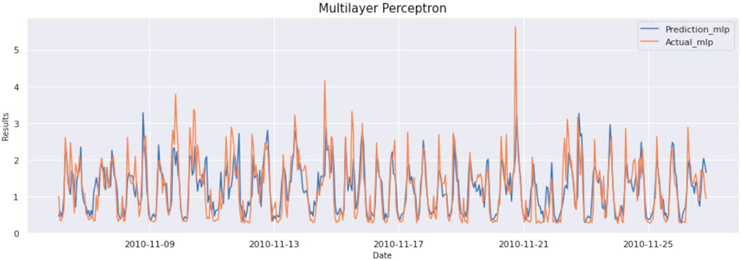
FIGURE 1. Prediction vs Actual result of Multilayer Perceptron (Household Electricity Data).

6.1.4 Long Short Term Memory

The architecture of LSTM is dependent on the types of layers and parameters adjustment of layers in the network. It consists of the LSTM layer, Dropout Layer (to prevent overfitting), and Dense layer to predict the output. After preliminary analysis of data parameters such as number of layers, neurons in each layer, loss functions, and optimization, algorithms are adjusted to give the best possible outcome.

Input data consists of a sliding window consisting of 24 data points (resampled to an hour). So, the input to the LSTM is 24 × 7 size data. There are a total of seven variables used to make the prediction. The proposed architecture for the LSTM layer with 100 neurons has been used for extracting patterns from the data. Model is trained with up to 100 epochs, and early stopping is used on data with a patience value of eight. It ensures that if there is a similar validation loss in each of eight consecutive epochs, then the model will stop running, and the most optimal weights will be stored as output. For optimizing the weights adam optimizer with a learning rate 0.0001 is used with a batch size of 256.

The result of this model is as MAE:0,382, MSE:262, and RMSE:512. The graph of actual vs predicted is as Figure 2.

FIGURE 2

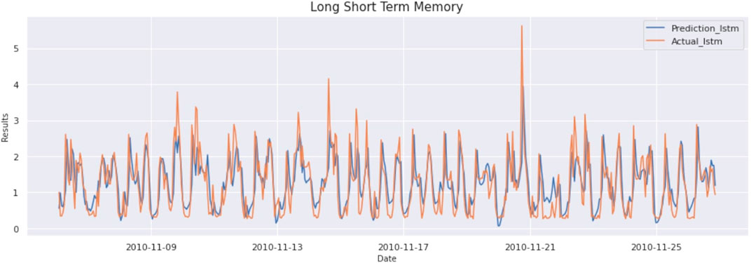
FIGURE 2. Prediction vs Actual result of LSTM model (Household Electricity Data).

6.1.5 CNN-Long Short Term Memory

The architecture of CNN-LSTM varies according to the number of layers, type of layers, and parameter adjustment in each layer. It consists of convolution layers, pooling layers, flatten layer, LSTM layers, and dense layer to predict the corresponding output. For convolution, the number of filters, size of the filter, and strides need to be adjusted. By adjustment of these parameters to an optimal level, accuracy can be significantly improved. To properly adjust the parameters of the model, data should be analyzed appropriately. As we already know that in CNN-LSTM, CNN layers use multiple variables and extract features between them hence improving time series forecasting significantly.

The correlation matrix shows a high correlation between different time-series variables with the variable we want to predict, i.e., Global Active Power (GAP). Input data consists of a sliding window consisting of 24 data points (resampled to an hour). So, the input to the CNN-LSTM is 24 × 7 size data. There are a total of seven variables used to make the prediction. The result of this model is as MAE:0,320, MSE:221, and RMSE:470. The graph of actual vs predicted is as Figure 3.

FIGURE 3

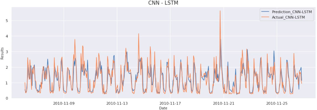
FIGURE 3. Prediction vs Actual result of CNN-LSTM model (Household Electricity Data).

6.1.6 VAR-CNN-Long Short Term Memory(VACL)

In this model architecture, first, we estimate VAR correctly on training data, and then we extract what VAR has learned and use it to refine the training of the CNN-LSTM process, giving better results. Firstly, to properly create a VAR model, data should be stationary. As already discussed, using ADFTest, it can be verified whether a time series is stationary or not. We applied the ADF Test on variables like global active power, global reactive power, voltage, global intensity, sub-metering 1, sub-metering 2, and sub-metering 3 with the null hypothesis that data has a unit root and is non-stationary. The ADF Test shows that all-time series are stationary, so differentiation is not needed for the series.

After doing this preliminary check, we need to find out the lag order, which can be calculated using AIC. All we need to do is to iterate through lag orders and find out the lag order with a minimum AIC score compared to its predecessors. In this case, 31 comes out to be the best lag order, as evident in Table 1. After getting the best order for VAR, we fit the VAR model on differentiated data. VAR can learn linear interdependencies in time series. This information is subtracted from raw data and gets the residuals that contain non-linear data.

TABLE 1

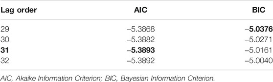
TABLE 1. Akaike information criterion on HouseHold data (Hebrail and Berard, 2012).

The architecture of the above model varies according to the number of layers, type of layers, and parameter adjustment in each layer. It consists of convolution layers, pooling layers, flatten layer, LSTM layers, and dense layer to predict the corresponding output. For convolution operation, the number of filters, filter size, and strides need to be adjusted. By adjustment of these parameters to an optimal level, accuracy can be significantly improved. To properly adjust the parameters of the model, data should be analyzed appropriately. Input provided to the model consists of a sliding window of 24 data points (resampled to an hour). So, the input to CNN-LSTM is 24 × 7 size data. The result of this model is as MAE:0,317, MSE:210, and RMSE:458. The graph of actual vs predicted is as Figure 4.

FIGURE 4

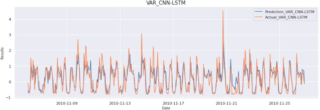
FIGURE 4. Prediction vs Actual result of VAR CNN-LSTM model (Household Electricity Data).

The combined results of all the algorithms are displayed in Table 2. We can observe that from the above table that both CNN-LSTM and the proposed approach perform well for given data, but the proposed model performed slightly better in terms of error metrics.

TABLE 2

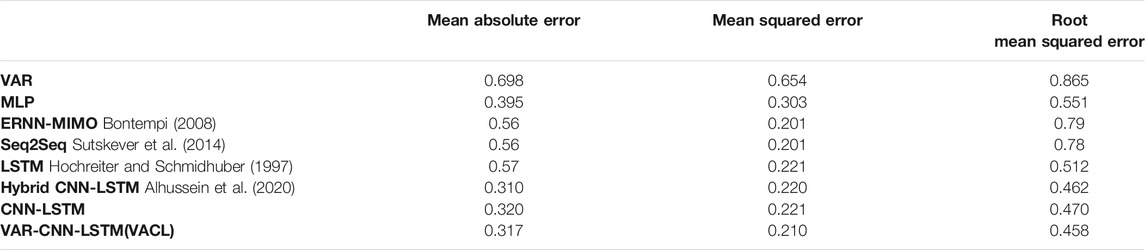
TABLE 2. Combined results of all the algorithms on Household Data (Hebrail and Berard, 2012).

6.2 Discussion on Ontario Power Demand Dataset

A multivariate time-series dataset consists of characteristics about Ontario Electricity Demand and corresponding Ontario Price and various other variables affecting these per 5-min sampling. It consists of ten time-series namely:

Ontario Price, Ontario Demand, Northwest, Northwest Temp, Northwest Dew Point Temp, Northwest Rel Hum, Northeast, Northeast Temp, Northeast Dew Point Temp, Northeast Rel Hum. The target is to forecast Ontario Price into the future by taking these variables. For the problem of price forecasting, two datasets from the Ontario region (Canada) are collected and combined from the following data sources:

1) ieso Power Data Directory. (ontario Energy Price-Dataset, 2020);

2) climate and weather data, Canada. (official website of the Government of Canada, 2020).

6.2.1 Preliminary Analysis

Preliminary analysis of data is being done, and patterns are evaluated, enabling us to make correct predictions. It is observed that time series follow seasonal patterns but there are irregular trend components. Figure 5 depicts that only the Ontario Demand time series should be considered for forecasting the Ontario Price time series. The reason is the approximately minimum coefficient value of correlation should be 0.3 for having a constructive relationship between each of these time series.

FIGURE 5

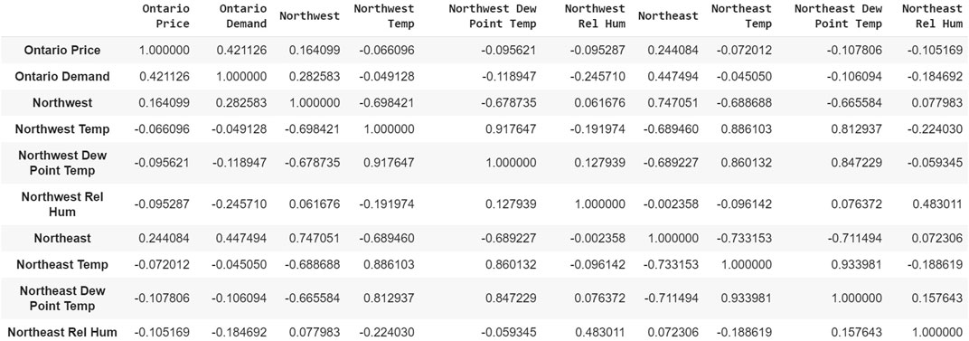
FIGURE 5. Correlation matrix (Ontario Demand Data).

6.2.2 Performance Comparison of Models

The best-fitted model to be used depends on available historical data, and the relationship between variables to be forecast. Experiments have been conducted for other neural network models consisting of MLP, LSTM, CNN-LSTM, etc., to establish the effectiveness of the proposed models, and results are evaluated with MSE and RMSE. Next, we will go through the architecture of each of these models and compare the results:

6.2.3 Multilayer Perceptron Model

Multilayer perceptron architecture depends on parameter adjustment and the number of hidden layers in the network. Multilayer perceptron consists of input layer consisting of input neurons, hidden layers, and output layer. The hidden layers consist of dense layers. We can optimize the number of neurons in hidden layers, learning algorithm, and loss functions based on input data. Here input data is resampled to convert it into hour-based sampling. Input data consists of a sliding window of 24 data points for which we will predict the next hour of the result. Input is 24 × 2 size data where 24 is the number of time steps, and 2 is the number of variables in each step.

The used architecture has one hidden layer with 100 neurons used to extract patterns from the data. Model is trained with up to 80 epochs, and early stopping is used on data with a patience value of eight. It ensures, if there is a similar validation loss in each of eight consecutive epochs, that the model will stop running, and the most optimal weights will be stored as output. ReLU activation is being used in the hidden layers, and for optimizing the weights, adam optimizer with learning rate, 0.000001 is used. The result of this model is as MAE:0,309, MSE:00204, and RMSE:0452. The graph of actual vs predicted is as Figure 6.

FIGURE 6

FIGURE 6. Prediction vs Actual result of Multilayer Perceptron (Ontario Demand Data).

6.2.4 Long Short Term Memory

The architecture of LSTM depends on the types of layers and parameters adjustment of layers in the network. It consists of the LSTM layer, Dropout Layer (to prevent overfitting), and Dense layer to predict the output. After preliminary analysis of data parameters such as the number of layers, neurons in each layer, loss functions, and optimization algorithms are adjusted to give the best possible outcome.

Input data consists of a sliding window consisting of 24 data points (resampled to an hour). So, the input to the LSTM is 24 × 2 size data. There are a total of two variables used to make the prediction. The proposed LSTM layer, each with 64 neurons, has been used for extracting patterns from the data. Model is trained with up to 100 epochs, and early stopping is used on data with a patience value of eight, which ensures if there is similar validation loss in each of eight consecutive epochs, then the model will stop running, and most optimal weights will be stored as output. The result of this model is as MAE:0,265, MSE:0015, and RMSE:0389. The graph of actual vs predicted is as Figure 7.

FIGURE 7

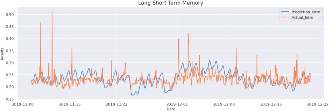
FIGURE 7. Prediction vs Actual result of LSTM model (Ontario Demand Data).

6.2.5 CNN-Long Short Term Memory

The architecture of CNN-LSTM varies according to the number of layers, layer type, and parameter adjustment in each layer. It consists of the convolution layers, pooling layers, flatten layer, LSTM layers, and dense layer to predict the corresponding output. For convolution operation, the number of filters, size of the filter, and strides need to be adjusted. By adjustment of these parameters to an optimal level, accuracy can be significantly improved. To properly adjust the parameters of the model, data should be analyzed appropriately.

It is known that in CNN-LSTM, CNN layers use multiple variables and extract features between them, improving time series forecasting significantly. As from the correlation matrix in Figure 5, it is observed that there is a high correlation between Ontario Price and Ontario Demand. Input data consists of a sliding window consisting of 24 data points (resampled to an hour). So, the input to the CNN-LSTM is 24 × 2 size data. There are a total of 2 variables used to make the prediction. The result of this model is as MAE:0,119, MSE:00068, and RMSE:02616. The graph of actual vs predicted is as Figure 8.

FIGURE 8

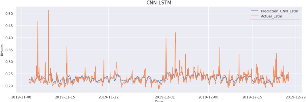
FIGURE 8. Prediction vs Actual result of CNNLSTM model (Ontario Demand Data).

6.2.6 VAR-CNN-Long Short Term Memory(VACL)

In this model architecture, we first estimate VAR correctly on training data, and then we extract what VAR has learned and use it to refine the training of the CNN-LSTM process. Firstly, to properly create a VAR model, we need to make data stationery, if not in the requisite format. As already discussed, using the ADFTest, we can check whether a time series is stationary or not. Results from the ADF Test show that every time-series are stationary, we do not need to differentiate the series.

After doing these preliminary checks, we need to find out the lag order, which can be calculated using AIC. All we need to do is to iterate through lag orders and find out the lag order with a minimum AIC score compared to its predecessors. In this case, 29 comes out to be the best lag order, as evident in this Table 3. After getting the best order for VAR, we fit the VAR model on differentiated data. VAR can learn linear interdependencies in time series. This information is subtracted from raw data to get the residuals which contain non-linear data as evident from Figure 9.

TABLE 3

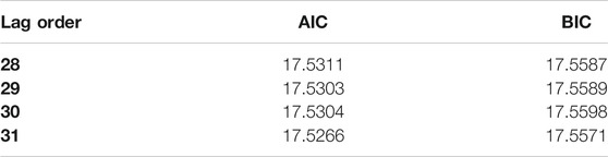
TABLE 3. Akaike information criterion on ontario demand data (ontario Energy Price-Dataset, 2020) (official website of the Government of Canada, 2020).

FIGURE 9

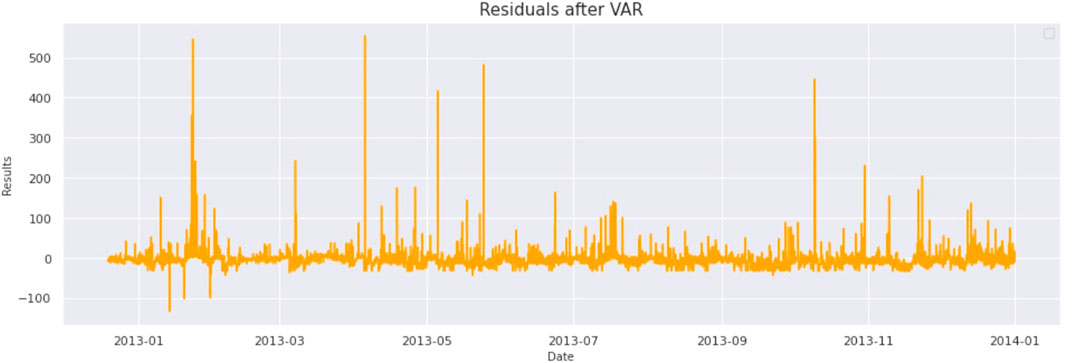
FIGURE 9. Residuals left after applying VAR (Ontario Demand Data).

After getting forecasting results from VAR, CNN-LSTM is trained on those forecasted results along with original data to learn all the intricacies from the data. The architecture of the CNN-LSTM model varies according to the number of layers, layer type, and parameter adjustment in each layer. It consists of convolution layers, pooling layers, flatten layer, LSTM layers, and dense layer to predict the corresponding output. For convolution operation, the number of filters, filter size, and strides need to be adjusted. By adjustment of these parameters to an optimal level, accuracy can be significantly improved. To properly adjust the parameters of the model, data should be analyzed appropriately. Input provided to the model consists of a sliding window of 24 data points (resampled to an hour). So, the input to CNN-LSTM is 24 × 2 size data as shown in Figure 10. The result of this model is as MAE:0,123, MSE:00054, and RMSE:0233. The graph of actual vs predicted is as Figure 11.

FIGURE 10

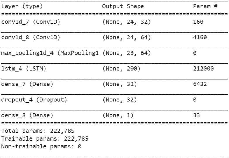
FIGURE 10. VAR CNN-LSTM model summary (Ontario Demand Data).

FIGURE 11

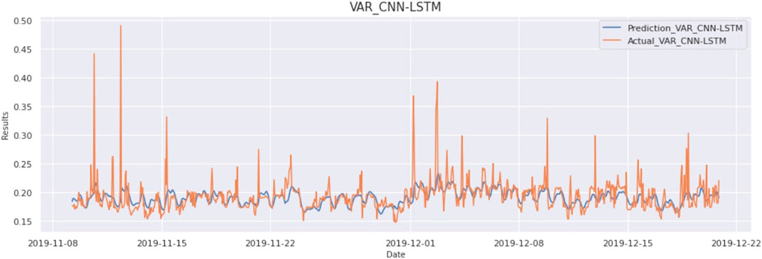
FIGURE 11. Prediction vs Actual result of VAR CNN-LSTM model (Ontario Demand Data).

The combined results of all the algorithms for Ontario Demand Data is displayed in Table 4. From the results of Table 4, it is clearly observed that the proposed VAR-CNN-LSTM(VACL) hybrid model has been compared with state of art models MV-KWNN(Talavera-Llames et al., 2019), MV-ANN(Hippert et al., 2001), ARIMAX (Box et al., 2011), VAR, MLP, LSTM and CNN-LSTM, and it outperforms all other models in terms of performance.

TABLE 4

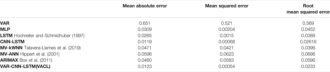
TABLE 4. Combined results of all the algorithms on Ontario Demand Data (ontario Energy Price-Dataset, 2020) (official website of the Government of Canada, 2020).

7 Conclusion and Future Scope

In this paper, the forecasting method for electricity load is investigated on a large dataset having linear and non-linear characteristics. We first formulated the problem as predicting the future term of multivariate time-series data, and then the proposed hybrid model VAR-CNN-LSTM(VACL) was deployed for efficient short-term power load forecasting. We have shown that the historical electrical load data is in the form of time series that consists of linear and non-linear components. Due to hybrid nature of the proposed model, the linear components were handled by VAR and residuals containing non-linear components by the combined CNN-LSTM layered architecture. The output efficiency was further enhanced by data preprocessing and analysis. With data preprocessing, the problem of missing values was solved, and data were normalized to bring values of the dataset to a common scale (Jaitley, 2019). From the data analysis, the correlation between variables have been discovered for, e.g., in household power consumption data, it was found that Global Active Power is correlated with all the variables in time series, so all variables wereused for forecasting. Since in Ontario Demand Dataset, only two variables were correlated, so all others were filtered out. The proposed method is modeled and tested on two publicly available datasets: Household Power Consumption Dataset and Ontario Demand dataset for short-term forecasting. The evaluation metrics used were MAE, MSE, and RMSE to show the effectiveness and errors respectively. From the results, it was established that the proposed hybrid VACL model performed better than other statistical and deep learning based techniques like VAR, CNN-LSTM, LSTM, MLP, and state-of-the-art model like MV-KWNN, MV-ANN and ARIMAX in all evaluation metrics.

One of the limitations of the proposed model was that determining all the hyperparameters like number of neurons, learning rate, number of epochs, batch size, etc., required great effort and time. As a future scope, more advanced hyperparameter optimization techniques may be used. Since the model has been tested for short-term load forecasting, the presented model will further analyze for the medium and long-term forecasting scenario.

Data Availability Statement

Publicly available datasets were analyzed in this study. This data can be found here: http://archive.ics.uci.edu/ml and https://www.ieso.ca/power-data.

Author Contributions

Conceptualization and Investigation: AS. Software and validation: RT and AV. Supervision, Writing-review and editing: PP and OPV.

Funding

Funding received from Research Council of Norway Grant No.: 280617, CPSEC and joint collaboration with Department of Science and Technology (DST), India for the Cyber Physical Security in Energy Infrastructure for Smart Cities (CPSEC) project under Smart Environments theme of Indo-Norwegian Call.

Conflict of Interest

The authors declare that the research was conducted in the absence of any commercial or financial relationships that could be construed as a potential conflict of interest.

Publisher’s Note

All claims expressed in this article are solely those of the authors and do not necessarily represent those of their affiliated organizations, or those of the publisher, the editors, and the reviewers. Any product that may be evaluated in this article, or claim that may be made by its manufacturer, is not guaranteed or endorsed by the publisher.

Acknowledgments

The work is supported by Department of Science and Technology(DST), India for the Cyber Physical Security in Energy Infrastructure for Smart Cities(CPSEC) project under Smart Environments theme of Indo-Norwegian Call.

References

Albawi, S., Mohammed, T. A., and Al-Zawi, S. (2017). “Understanding of a Convolutional Neural Network,” in 2017 International Conference on Engineering and Technology (ICET), Antalya, Turkey, August 21–23, 2017, 1–6. doi:10.1109/ICEngTechnol.2017.8308186

CrossRef Full Text | Google Scholar

Alhussein, M., Aurangzeb, K., and Haider, S. I. (2020). Hybrid Cnn-Lstm Model for Short-Term Individual Household Load Forecasting. IEEE Access 8, 180544–180557. doi:10.1109/ACCESS.2020.3028281

CrossRef Full Text | Google Scholar

Babu, C. N., and Reddy, B. E. (2014). A Moving-Average Filter Based Hybrid ARIMA-ANN Model for Forecasting Time Series Data. Appl. Soft Comput. 23, 27–38. doi:10.1016/j.asoc.2014.05.028

CrossRef Full Text | Google Scholar

Bedi, J., and Toshniwal, D. (2019). Deep Learning Framework to Forecast Electricity Demand. Appl. Energ. 238, 1312–1326. doi:10.1016/j.apenergy.2019.01.113

CrossRef Full Text | Google Scholar

Bendaoud, N. M. M., and Farah, N. (2020). Using Deep Learning for Short-Term Load Forecasting. Neural Comput. Applic 32, 15029–15041. doi:10.1007/s00521-020-04856-0

CrossRef Full Text | Google Scholar

Bikcora, C., Verheijen, L., and Weiland, S. (2018). Density Forecasting of Daily Electricity Demand with Arma-Garch, Caviar, and Care Econometric Models. Sustainable Energ. Grids Networks 13, 148–156. doi:10.1016/j.segan.2018.01.001

CrossRef Full Text | Google Scholar

Biller, B., and Nelson, B. L. (2003). Modeling and Generating Multivariate Time-Series Input Processes Using a Vector Autoregressive Technique. ACM Trans. Model. Comput. Simul. 13, 211–237. doi:10.1145/937332.937333

CrossRef Full Text | Google Scholar

Bontempi, G. (2008). Long Term Time Series Prediction with Multi-Input Multi-Output Local Learning. Proc. 2nd ESTSP, 145–154.

Google Scholar

Bourdeau, M., Zhai, X. q., Nefzaoui, E., Guo, X., and Chatellier, P. (2019). Modeling and Forecasting Building Energy Consumption: A Review of Data-Driven Techniques. Sustain. Cities Soc. 48, 101533. doi:10.1016/j.scs.2019.101533

CrossRef Full Text | Google Scholar

Box, G. E., Jenkins, G. M., and Reinsel, G. C. (2011). Time Series Analysis: Forecasting and Control, Vol. 734. John Wiley & Sons.

Google Scholar

Chatfield, C. (1996). The Analysis of Time Series – an Introduction. Chapman & Hall.

Google Scholar

Chen, T.-B., and Soo, V.-W. (1996). “A Comparative Study of Recurrent Neural Network Architectures on Learning Temporal Sequences,” in International Conference on Neural Networks, Washington, DC, June 3–6, 1996 (IEEE), 1945–1950.4.

Google Scholar

Chniti, G., Bakir, H., and Zaher, H. (2017). “E-commerce Time Series Forecasting Using Lstm Neural Network and Support Vector Regression,” in Proceedings of the International Conference on Big Data and Internet of Thing - BDIOT2017. doi:10.1145/3175684.3175695

CrossRef Full Text | Google Scholar

Choi, H. K. (2018). Stock price Correlation Coefficient Prediction with ARIMA-LSTM Hybrid Model. CoRR abs/1808.01560.

Google Scholar

Choi, J. Y., and Lee, B. (20182018). Combining Lstm Network Ensemble via Adaptive Weighting for Improved Time Series Forecasting. Math. Probl. Eng. 2018, 1–8. doi:10.1155/2018/2470171

CrossRef Full Text | Google Scholar

[Dataset] Cohen, I. (2021). Time Series-Introduction. A Time Series Is a Series of data– by Idit Cohen – towards Data Science. Available at: https://towardsdatascience.com/time-series-introduction-7484bc25739a (Accessed on 04 06, 2021).

Google Scholar

Du, P., Wang, J., Yang, W., and Niu, T. (2019). A Novel Hybrid Model for Short-Term Wind Power Forecasting. Appl. Soft Comput. 80, 93–106. doi:10.1016/j.asoc.2019.03.035

CrossRef Full Text | Google Scholar

Elman, J. L. (1990). Finding Structure in Time. Cogn. Sci. 14, 179–211. doi:10.1207/s15516709cog1402_1

CrossRef Full Text | Google Scholar

[Dataset] Erica (2021). Introduction to the Fundamentals of Time Series Data and Analysis - Aptech. Available at: https://www.aptech.com/blog/introduction-to-the-fundamentals-of-time-series-data-and-analysis/(Accessed on Jun 19, 2021).

Google Scholar

Fukushima, K. (1980). Neocognitron: A Self-Organizing Neural Network Model for a Mechanism of Pattern Recognition Unaffected by Shift in Position. Biol. Cybernetics 36, 193–202. doi:10.1007/bf00344251

CrossRef Full Text | Google Scholar

Gasparin, A., Lukovic, S., and Alippi, C. (2019). Deep Learning for Time Series Forecasting: The Electric Load Case. CoRR abs/1907.09207.

Google Scholar

Hartmann, C., Hahmann, M., Habich, D., and Lehner, W. (2017). “Csar: The Cross-Sectional Autoregression Model,” in IEEE International Conference on Data Science and Advanced Analytics (DSAA), Tokyo, Japan, October 19–21, 2017, 232–241. doi:10.1109/DSAA.2017.27

CrossRef Full Text | Google Scholar

Hebrail, G., and Berard, A. (2012). Individual Household Electric Power Consumption Data Set. Irvine: University of California.

Google Scholar

Hippert, H. S., Pedreira, C. E., and Souza, R. C. (2001). Neural Networks for Short-Term Load Forecasting: a Review and Evaluation. IEEE Trans. Power Syst. 16, 44–55. doi:10.1109/59.910780

CrossRef Full Text | Google Scholar

Hochreiter, S., and Schmidhuber, J. (1997). Long Short-Term Memory. Neural Comput. 9, 1735–1780. doi:10.1162/neco.1997.9.8.1735

PubMed Abstract | CrossRef Full Text | Google Scholar

Ibrahim, H., Ilinca, A., and Perron, J. (2008). Energy Storage Systems-Characteristics and Comparisons. Renew. Sustain. Energ. Rev 12 (5), 1221e50. doi:10.1016/j.rser.2007.01.023

CrossRef Full Text | Google Scholar

[Dataset] Jaitley, U. (2019). Why Data Normalization Is Necessary for Machine Learning Models. Available at: https://medium.com/@urvashilluniya/why-data-normalization-is-necessary-for-machine-learning-models-681b65a05029".

Google Scholar

Jordan, M. I. (1990). “Attractor Dynamics and Parallelism in a Connectionist Sequential Machine,” in Artificial Neural Networks: Concept Learning. Artificial Neural Network:Concept Learning, 112–127.

Google Scholar

Khwaja, A. S., Anpalagan, A., Naeem, M., and Venkatesh, B. (2020). Joint Bagged-Boosted Artificial Neural Networks: Using Ensemble Machine Learning to Improve Short-Term Electricity Load Forecasting. Electric Power Syst. Res. 179, 106080. doi:10.1016/j.epsr.2019.106080

CrossRef Full Text | Google Scholar

Kim, T.-Y., and Cho, S.-B. (2019). Predicting Residential Energy Consumption Using Cnn-Lstm Neural Networks. Energy 182, 72–81. doi:10.1016/j.energy.2019.05.230

CrossRef Full Text | Google Scholar

Lütkepohl, H. (2013). Introduction to Multiple Time Series Analysis. Springer Science & Business Media.

Google Scholar

Ma, X., Jin, Y., and Dong, Q. (2017). A Generalized Dynamic Fuzzy Neural Network Based on Singular Spectrum Analysis Optimized by Brain Storm Optimization for Short-Term Wind Speed Forecasting. Appl. Soft Comput. 54, 296–312. doi:10.1016/j.asoc.2017.01.033

CrossRef Full Text | Google Scholar

Mahalakshmi, G., Sridevi, S., and Rajaram, S. (2016). “A Survey on Forecasting of Time Series Data,” in 2016 International Conference on Computing Technologies and Intelligent Data Engineering (ICCTIDE’16), Kovilpatti, India, January 7–9, 2016 (IEEE), 1–8. doi:10.1109/icctide.2016.7725358

CrossRef Full Text | Google Scholar

Miller, N., Guru, D., and Clark, K. (2009). Wind Generation. IEEE Ind. Appl. Mag. 15, 54–61. doi:10.1109/mias.2009.931820

CrossRef Full Text | Google Scholar

Nair, V., and Hinton, G. E. (2010). “Rectified Linear Units Improve Restricted Boltzmann Machines,” in Icml.

Google Scholar

[Dataset] official website of the Government of Canada (2020). Historical Climate Data (Accessed on Feburary 15, 2020).

Google Scholar

[Dataset] Olah, C. (2013). Understanding Lstm Networks.

Google Scholar

[Dataset] OMIE-Dataset (2020). Day-ahead Market Hourly Prices in spain. Available at: https://www.omie.es/en/file-access-list?parents%5B0%5D=/&parents%5B1%5D=Day-ahead%20Market&parents%5B2%5D=1.%20Prices&dir=%20Day-ahead%20market%20hourly%20prices%20in%20Spain&realdir=marginalpdbc (Accessed May 15, 2020).

Google Scholar

[Dataset] ontario Energy Price-Dataset (2020). Hourly ontario Energy price (Hoep). Available at: https://www.ieso.ca/en/Power-Data/Data-Directory (Accessed on Feburary 15, 2020).

Google Scholar

[Dataset] Prabhakaran, S. (2020). Vector Autoregression (Var) - Comprehensive Guide with Examples in python. Available at: https://www.machinelearningplus.com/time-series/vector-autoregression-examples-python/.

Google Scholar

Rahman, A., Srikumar, V., and Smith, A. D. (2018). Predicting Electricity Consumption for Commercial and Residential Buildings Using Deep Recurrent Neural Networks. Appl. Energ. 212, 372–385. doi:10.1016/j.apenergy.2017.12.051

CrossRef Full Text | Google Scholar

Rashid, T., Huang, B., Kechadi, T., and Gleeson, B. (2009). Auto-regressive Recurrent Neural Network Approach for Electricity Load Forecasting 3, 36–44.

Google Scholar

[Dataset] Rawat, W., and Wang, Z. (2017). Deep Convolutional Neural Networks for Image Classification: A Comprehensive Review, Neural Computing.

Google Scholar

Sherstinsky, A. (2018). Fundamentals of Recurrent Neural Network (Rnn) and Long Short-Term Memory (Lstm) Network. New York: John Wiley & Sons.

Google Scholar

Shi, H., Xu, M., and Li, R. (2017). Deep Learning for Household Load Forecasting—A Novel Pooling Deep Rnn. IEEE Trans. Smart Grid 9, 5271–5280. doi:10.1109/TSG.2017.2686012

CrossRef Full Text | Google Scholar

Shiblee, M., Kalra, P. K., and Chandra, B. (2009). “Time Series Prediction with Multilayer Perceptron (Mlp): A New Generalized Error Based Approach,” in Advances in Neuro-Information Processing Lecture Notes in Computer Science, Auckland, New Zealand, November 25–28, 2008, 37–44. doi:10.1007/978-3-642-03040-6_5

CrossRef Full Text | Google Scholar

Shirzadi, N., Nizami, A., Khazen, M., and Nik-Bakht, M. (2021). Medium-Term Regional Electricity Load Forecasting through Machine Learning and Deep Learning. Designs 5, 27. doi:10.3390/designs5020027

CrossRef Full Text | Google Scholar

Siami-Namini, S., Tavakoli, N., and Siami Namin, A. (2018). “A Comparison of Arima and Lstm in Forecasting Time Series,” in 17th IEEE International Conference on Machine Learning and Applications (ICMLA), Orlando, FL, December 17–20, 2018, 1394–1401. doi:10.1109/ICMLA.2018.00227

CrossRef Full Text | Google Scholar

Sinha, A., Tayal, R., Vyas, R., and Vyas, O. (2021). “Operational Flexibility with Statistical and Deep Learning Model for Electricity Load Forecasting,” in Lecture Notes in Electrical Engineering (LNEE) (Springer).

Google Scholar

Sorjamaa, A., and Lendasse, A. (2006). Time Series Prediction Using Dirrec Strategy. Esann (Citeseer) 6, 143–148.

Google Scholar

Stoll, H. G., and Garver, L. J. (1989). Least-cost Electric Utility Planning. New York: Electrical Energy Systems; Electrical Companies.

Google Scholar

Sutskever, I., Vinyals, O., and Le, Q. V. (2014). “Sequence to Sequence Learning with Neural Networks,” in Advances in Neural Information Processing Systems, 3104–3112.

Google Scholar

Taieb, S. B., Bontempi, G., Sorjamaa, A., and Lendasse, A. (2009). “Long-term Prediction of Time Series by Combining Direct and Mimo Strategies,” in International Joint Conference on Neural Networks, Atlanta, GA, June 14–19, 2009 (IEEE), 3054–3061. doi:10.1109/ijcnn.2009.5178802

CrossRef Full Text | Google Scholar

Talavera-Llames, R., Pérez-Chacón, R., Troncoso, A., and Martínez-Álvarez, F. (2019). Mv-kwnn: A Novel Multivariate and Multi-Output Weighted Nearest Neighbours Algorithm for Big Data Time Series Forecasting. Neurocomputing 353, 56–73. doi:10.1016/j.neucom.2018.07.092

CrossRef Full Text | Google Scholar

Wang, J., Yu, L.-C., Lai, K. R., and Zhang, X. (2016). “Dimensional Sentiment Analysis Using a Regional CNN-LSTM Model,” in Proceedings of the 54th Annual Meeting of the Association for Computational Linguistics (Volume 2: Short Papers), Berlin, Germany, August 7–12, 2016 (Berlin, Germany: Association for Computational Linguistics), 225–230. doi:10.18653/v1/P16-2037

CrossRef Full Text | Google Scholar

[Dataset] Wikipedia (2021). Time Series Wikipedia. Available at: https://en.wikipedia.org/wiki/Time_series (Accessed on 0619, 2021).

Google Scholar

Wu, F., Cattani, C., Song, W., and Zio, E. (2020). Fractional Arima with an Improved Cuckoo Search Optimization for the Efficient Short-Term Power Load Forecasting. Alexandria Eng. J. 59, 3111–3118. doi:10.1016/j.aej.2020.06.049

CrossRef Full Text | Google Scholar

Wu, Z., Zhao, X., Ma, Y., and Zhao, X. (2019). A Hybrid Model Based on Modified Multi-Objective Cuckoo Search Algorithm for Short-Term Load Forecasting. Appl. Energ. 237, 896–909. doi:10.1016/j.apenergy.2019.01.046

CrossRef Full Text | Google Scholar

Xiao, L., Shao, W., Wang, C., Zhang, K., and Lu, H. (2016). Research and Application of a Hybrid Model Based on Multi-Objective Optimization for Electrical Load Forecasting. Appl. Energ. 180, 213–233. doi:10.1016/j.apenergy.2016.07.113

CrossRef Full Text | Google Scholar

Yan, K., Wang, X., Du, Y., Jin, N., Huang, H., and Zhou, H. (2018). Multi-step Short-Term Power Consumption Forecasting with a Hybrid Deep Learning Strategy. MDPI J. Energies. doi:10.3390/en11113089

CrossRef Full Text | Google Scholar

Yao, X. (1993). A Review of Evolutionary Artificial Neural Networks. Int. J. Intell. Syst. 8, 539–567. doi:10.1002/int.4550080406

CrossRef Full Text | Google Scholar