A Fast Tomographic Reconstruction Method for Flame Temperature Distribution Measurement Based on Direct Solution Algorithm

Introduction

Thrust-to-weight ratio is a comprehensive index to measure the performance level and working ability of aero engines. One of the main ways to improve the thrust-to-weight ratio of modern aero engines is to increase the outlet temperature of the combustion chamber (Zhang et al., 2019). As the temperature rises, turbine blades and vanes need to bear a greater thermal load. The huge thermal gradient causes severe thermal stress and strain on the blades, which greatly reduces the creep life of the blades, and leads to ablation, fracture and failure of the blades (Marahleh et al., 2006). Real-time monitoring and obtaining accurate combustion chamber outlet temperature can respond to local temperature sudden changes in the engine in a timely manner, which is of great significance for the safety of aero-engine operation and prolonged service life (Li et al., 2006; He et al., 2019; Gamil et al., 2020).

Due to the shortcomings of thermocouple and other contact temperature measurement, such as slow dynamic response, interference with combustion field, narrow temperature measurement range, only point measurement, high-temperature oxidation, etc., it is not suitable for cutting-edge combustion chambers under high temperature, high pressure, and high-speed conditions (Yang et al., 2015; Jenkins et al., 2020; Zhang et al., 2016; Lian et al., 2017). In recent years, the flame temperature distribution reconstruction technology based on radiation images has received extensive attention from researchers all over the world (Neuer et al., 2001; Sun et al., 2018; Qi et al., 2019; Zhao et al., 2017; Hossain et al., 2013; Niu et al., 2015). It has the advantages of non-invasiveness and no need for external excitation sources and is more suitable for the measurement of the exit temperature distribution of the combustion chamber of aero engines.

The radiation image method for temperature measurement utilizes flame radiation information from different directions to reconstruct the flame temperature field, and the use of a reasonable reconstruction algorithm is beneficial to improve the efficiency and accuracy of temperature distribution reconstruction. Generally, the number of grids in the reconstruction area will affect the efficiency of the reconstruction algorithm. As the number of grids increases, the difficulty and time to solve the ill-conditioned equations transformed from the inverse radiation problem tend to increase exponentially, which is difficult to meet the current demand for rapid reconstruction of the exit temperature of the combustion chamber of aero engines.

To solve the above-mentioned problems, Zhou et al. (2002) used an improved Tikhonov regularization algorithm to reconstruct a three-dimensional temperature distribution of ${\mathit{N}}_{\mathit{x}}\times {\mathit{N}}_{\mathit{y}}\times {\mathit{N}}_{\mathit{z}}=10\times 10\times 10$ from the flame image obtained by the CCD camera, which proved the robustness of the algorithm, but the reconstruction efficiency is not studied. Liu et al. (2010) used the Least Square QR decomposition (LSQR) algorithm to achieve a two-dimensional temperature distribution reconstruction with a discrete area of ${\mathit{N}}_{\mathit{x}}\times {\mathit{N}}_{\mathit{y}}=10\times 10$ based on an 8-camera system combined with the Monte Carlo method. However, if the LSQR algorithm is directly used for large-scale ill-conditioned problems, there will be a “semi-convergence” problem, which will affect the accuracy and reconstruction time. Qiu et al. (2014) combined the Tikhonov regularization algorithm and generalized truncated singular value decomposition hybrid algorithm (TR-GSVD) to reconstruct the temperature distribution in the discrete area of ${\mathit{N}}_{\mathit{x}}\times {\mathit{N}}_{\mathit{y}}\times {\mathit{N}}_{\mathit{z}}=10\times 10\times 12$ in the furnace, and the reconstruction time is about 2s. Cai et al. (2013) reconstructed the flame temperature distribution with a grid number of ${\mathit{N}}_{\mathit{x}}\times {\mathit{N}}_{\mathit{y}}\times {\mathit{N}}_{\mathit{z}}=54\times 54\times 10$ based on chemiluminescence tomography technology, using Algebraic Reconstruction Technique (ART) and minimization algorithm combined with regularization technology. Numerical simulations and experiments have verified the effectiveness of the method. However, the low efficiency of the “line-by-line correction” of the ART algorithm will affect the reconstruction time. Huang et al. (2018) used the improved Landweber algorithm to reconstruct the three-dimensional temperature distribution of the absorbing and scattering flame based on the light field imaging technology. But it still takes 2.5 s to reconstruct the temperature distribution with the number of grids ${\mathit{N}}_{\phi }\times {\mathit{N}}_{\mathit{r}}\times {\mathit{N}}_{\mathit{l}}=1\times 20\times 20$. The above-mentioned traditional algorithms have achieved certain results in the reconstruction of the temperature distribution, but the calculation time for the reconstruction of the temperature distribution with a large number of grids is generally too longer. Therefore, it is necessary to develop a flame temperature distribution reconstruction algorithm that greatly improves the reconstruction efficiency under the premise of ensuring accuracy and is less affected by the increase in the number of grids.

In this paper, based on the CCD camera imaging and flame radiative transfer model, the rapid reconstruction method of absorbing and scattering flame temperature distribution is carried out. It takes the generalized source term finite volume method as the model of the forward problem and the proposed direct solution algorithm as the inverse method for reconstructing the temperature distribution. Two numerical cases of flame temperature distribution reconstruction are designed to illustrate the performance of the proposed direct solution algorithm compared with the current main tomographic algorithms, such as Simultaneous Algebraic Reconstruction Technique (SART), LSQR, and Non-Negative Least Squares QR-factorization (NNLS) algorithm.

Theories and Methods

Forward Model

In the radiation image method for temperature measurement, as shown in Figure 1, an ideal thin lens model can be used to describe the imaging process of light from the object space passing through the lens to the camera detector pixels. The light entering the camera is characterized by the line between the center of the CCD pixel and the optical center of the lens. Considering that the flame is a semi-transparent object, the light will pass through the flame. When the deflection effect of the flame refractive index gradient on the light is not considered, the radiation of the flame voxel through which the light passes all contributes to the gray value of the pixel. Therefore, it is necessary to record the number of flame voxels that each detection light passes through, and the distance traveled in the voxel. According to the generalized source term finite volume method (Zhang et al., 2017), the radiation energy received on each pixel can be calculated by the following formula:

$\mathit{I}\left({\mathit{r}}_{\mathit{p}},\mathbf{\Omega }\right)=\mathit{S}\left({\mathit{r}}_{\mathit{n}},\mathbf{\Omega }\right)\left[1-\exp \left(-{\beta }_{\mathit{n}}\Delta {\mathit{s}}_{\mathit{n}}\right)\right]+{\displaystyle \sum }_{\mathit{i}=1}^{\mathit{n}-1}\mathit{S}\left({\mathit{r}}_i,\mathbf{\Omega }\right)\left[\mathit{exp}\left(-{\displaystyle \sum }_{\mathit{j}=\mathit{i}+1}^{\mathit{n}}{\beta }_{\mathit{j}}\Delta {\mathit{s}}_{\mathit{j}}\right)-\mathit{exp}\left(-{\displaystyle \sum }_{\mathit{j}=\mathit{i}}^{\mathit{n}}{\beta }_{\mathit{j}}\Delta {\mathit{s}}_{\mathit{j}}\right)\right](1)$

where $\mathit{I}\left({\mathit{r}}_{\mathit{p}},\mathbf{\Omega }\right)$ is the radiation intensity along the direction $\mathbf{\Omega }$ at the position ${\mathit{r}}_p$. $n$ is the total number of the flame voxel that the light passes through. $S\left({\mathit{r}}_i,\mathbf{\Omega }\right)$ is the generalized source term of the $n \text{th}$ voxel along the direction $\mathbf{\Omega }$. $\beta$ is the extinction coefficient of the flame. $\text{Δs}$ is the distance that the light travels through the flame voxel, witch can be determined by the reverse tracing of the light.

FIGURE 1

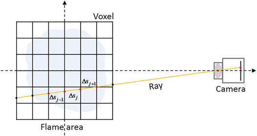
FIGURE 1. The schematic diagram of flame radiation imaging for temperature measurement.

Since the propagation speed of light is much greater than the equilibrium speed of temperature, the radiative transfer of flame in radiation image method for temperature measurement can be expressed by the steady-state radiative transfer equation (Qi et al., 2015):

$\frac{\mathit{dI}\left(\mathit{r},\mathbf{\Omega }\right)}{\beta \mathit{ds}}=-\mathit{I}\left(\mathit{r},\mathbf{\Omega }\right)+\left(1-\omega \right){\mathit{I}}_{\mathit{b}}\left(\mathit{r}\right)+\frac{\omega }{4\pi }{\displaystyle \underset{4\pi }{\int }\mathit{I}\left(\mathit{r},{\mathbf{\Omega }}^{\prime }\right)\Phi \left({\mathbf{\Omega }}^{\prime },\mathbf{\Omega }\right)\mathit{d}\mathbf{\Omega }}(2)$

where $\mathit{I}\left(\mathit{r},\mathbf{\Omega }\right)$ is the radiative intensity along the direction $\mathbf{\Omega }$ at the flame voxel $\mathit{r}$. ${\mathit{I}}_{\mathit{b}}\left(\mathit{r}\right)$ is the black body radiative intensity at the flame voxel $\mathit{r}$. $\omega$ is scattering albedo of the flame. $\Phi \left({\mathbf{\Omega }}^{\prime },\mathbf{\Omega }\right)$ is the scattering phase function, where $\mathbf{\Omega }\prime$ is the incident direction and $\mathbf{\Omega }$ is the scattering direction. $\mathbf{\Omega }$ is the solid angle.

The second and third terms on the right side of Eq. (2) represent emission-enhanced and scattering-enhanced terms, respectively. The sum of the second and third terms can be defined as the generalized source term.

$\mathit{S}\left(\mathit{r},\mathbf{\Omega }\right)=\left(1-\omega \right){\mathit{I}}_{\mathit{b}}\left(\mathit{r}\right)+\frac{\omega }{4\pi }{\displaystyle \underset{4\pi }{\int }\mathit{I}\left(\mathit{r},{\mathbf{\Omega }}^{\prime }\right)\Phi \left({\mathbf{\Omega }}^{\prime },\mathbf{\Omega }\right)\mathit{d}\mathbf{\Omega }}(3)$

Each detected light of the camera can establish as an equation using Eq. (1), then all detected light of the camera can form reconstruction equations. The generalized source term distribution can be obtained through the inversion calculation of the reconstruction equations. After substituting the generalized source term, the finite volume method can be used to calculate the black body radiative intensity of each flame voxel, and then the temperature of each flame voxel can be obtained by Planck’s law.

$\begin{array}{cccc}\mathit{A}\cdot \mathit{S}=\mathit{I},& \mathit{A}\in {\mathrm{ℝ}}^{\mathit{M}\times \mathit{N}},& \mathit{S}\in {\mathrm{ℝ}}^{\mathit{N}},& \mathit{I}\in {\mathrm{ℝ}}^{\mathit{M}}\end{array}(4)$

where $A$ is the coefficient matrix of the reconstruction equations, which is related to the flame extinction coefficient and the optical path of the light passing through the voxels. $S$ is the generalized source term vector. $I$ is the flame radiative intensity distribution received by the CCD camera. $M$ and $N$ are the total number of detected lights and flame voxels.

Inversion Principle

The dimension of the coefficient matrix $A$ in the reconstruction equations is determined by the dimensions of the unknowns vector $S$ and the measured value vector $I$. Because the current camera resolution is relatively large (usually millions), resulting in a huge dimension of the coefficient matrix. This leads to low solution efficiency. However, the solution process can be optimized by analyzing the characteristics of the coefficient matrix. In order to facilitate the demonstration, a two-dimensional flame and linear CCD are used to analyze the flame temperature distribution reconstruction in this paper, as shown in Figure 2.

FIGURE 2

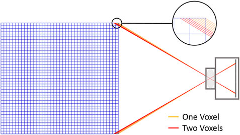
FIGURE 2. The schematic diagram of light propagation in the flame voxel.

According to Eq. (1), if the light passes through the flame voxel, the elements in the corresponding coefficient matrix are non-zero. If non-zero elements of the coefficient matrix are represented by blue dots, and zero elements of the coefficient matrix are represented by blanks, the coefficient matrix can be represented as Figure 3. It can be seen that the coefficient matrix $A$ is very sparse. There are several rows of coefficient matrix containing only one non-zero element, such as rows 1, 2, $\cdots$ , 6, M-5, M-4, $\cdots$ , M. It means that a specific unknown generalized source term value can be solved using one equation and one measured value. Due to the proximity of the voxels in space, many rows which contain two non-zero elements and one non-zero element share the same element. For example, row 6 and row 7 share a non-zero element 40. Therefore, the unknowns obtained in the previous calculation can be used to substitute back to a new row for elimination. Using this “solving-substitution” model, only a few equations need to be calculated each time to gradually complete the solution of large-scale linear equations, so that a few unknown equations can be calculated all the time to gradually complete the solution of large-scale coefficient equations. Considering that there are multiple rays of light passing through the same flame voxel at the same time, in order to reduce the influence of measurement error, multiple equations can be solved at the same time to obtain the least square solution of the same non-zero element. For example, rows 1, 2, 3, 4, 5, and 6 can form a sub-matrix to solve the 40th unknown generalized radiation source term.

FIGURE 3

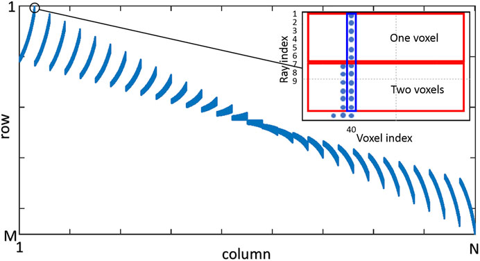
FIGURE 3. The schematic diagram of the element characteristics of the coefficient matrix $A$.

Since the reconstruction method proposed in this paper is to solve a certain unknown parameter each time directly, this method is called Direct Solution algorithm. The procedure for implementing the Direct Solution algorithm is described as the following steps, and the flowchart is shown in Figure 4.

FIGURE 4

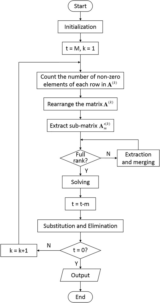
FIGURE 4. The flowchart of the direct solution algorithm.

Step 1. Input the coefficient matrix ${\mathit{A}}^{\left(\mathit{k}\right)}$ and count the number of non-zero elements and corresponding positions in each row.

Step 2. According to the counted number of non-zero elements, arrange the row vectors of the coefficient matrix in ascending order to form a new coefficient matrix ${\mathit{A}}^{\left(\mathit{k}\right)}$.

Step 3. Extract the row vectors containing the least specific non-zero element ${\mathit{a}}_{\mathit{i},\mathit{j}}$ from the matrix to form the solving sub-matrix $A_{\mathit{m}}^{\prime \left(\mathit{k}\right)}$, and the remaining part form the candidate sub-matrix $A_{\mathit{n}}^{\prime \left(\mathit{k}\right)}$.

Step 4. Check whether the solving sub-matrix $A_{\mathit{m}}^{\prime \left(\mathit{k}\right)}$ is full rank. If it is not full rank, go to Step 5. If it is full rank, go to Step 6.

Step 5. Extract the row vectors containing element ${\mathit{a}}_{\mathit{i},\mathit{j}}$ and the least non-zero elements from the candidate sub-matrix $A_n^{\text{'}\left(k\right)}$. Combine them with the solving sub-matrix $A_{\mathit{m}}^{\prime \left(\mathit{k}\right)}$ to form a new solving sub-matrix $A_{\mathit{m+t}}^{\prime \left(\mathit{k}\right)}$ and the remaining candidate sub-matrix constitutes a new candidate sub-matrix $A_{\mathit{m-t}}^{\prime \left(\mathit{k}\right)}$. Then go to Step 4.

Step 6. Use the LSQR algorithm to solve the sub-matrix $A_{\mathit{m}}^{\prime \left(\mathit{k}\right)}$. Substitute the calculation result back into the candidate sub-matrix $A_n^{\text{'}\left(k\right)}$. Eliminate the solved elements in the candidate sub-matrix to form a new coefficient matrix ${\mathit{A}}^{\left(\mathit{k}+1\right)}$. Loop to Steps 1 until all unknowns are obtained.

Results and Discussions

Evaluation Criterion

In order to evaluate the performance of the Direct Solution algorithm proposed in this paper, several common traditional reconstruction algorithms of flame temperature distribution are selected for comparison, such as SART (Liu et al., 2017), LSQR (Liu et al., 2010), NNLS (Li et al., 2019) algorithms. In terms of reconstruction accuracy, the following criteria are used for evaluation (Resnick et al., 1985): 1) The normalized mean square distance, $q$; 2) The normalized average absolute distance, $\mathit{r}$; The worst-case distance, $e$. The specific expressions are shown in Eqs (5)–(7).

$\mathit{r}={\displaystyle \sum _{\mathit{i}=1}^{\mathit{N}}{\displaystyle \sum _{\mathit{j}=1}^{\mathit{N}}\left|{\mathit{T}}_{\mathit{i},\mathit{j}}-{\mathit{R}}_{\mathit{i},\mathit{j}}\right|/{\displaystyle \sum _{\mathit{i}=1}^{\mathit{N}}{\displaystyle \sum _{\mathit{j}=1}^{\mathit{N}}\left|{\mathit{T}}_{\mathit{i},\mathit{j}}\right|}}}}(5)$

$\mathit{q}={\displaystyle \sum _{\mathit{i}=1}^{\mathit{N}}{\displaystyle \sum _{\mathit{j}=1}^{\mathit{N}}{\left({\mathit{T}}_{\mathit{i},\mathit{j}}-{\mathit{R}}_{\mathit{i},\mathit{j}}\right)}^2/{\displaystyle \sum _{\mathit{i}=1}^{\mathit{N}}{\displaystyle \sum _{\mathit{j}=1}^{\mathit{N}}{\left({\mathit{T}}_{\mathit{i},\mathit{j}}-\overline{\mathit{T}}\right)}^2}}}}(6)$

$\begin{array}{cc}\mathit{e}=\underset{\begin{array}{c}1\le \mathit{i}\le \left[\frac{\mathit{N}}{2}\right]\\ 1\le \mathit{j}\le \left[\frac{\mathit{N}}{2}\right]\end{array}}{\max }\left|{\mathit{M}}_{\mathit{i},\mathit{j}}-{\mathit{E}}_{\mathit{i},\mathit{j}}\right|,& \{\begin{array}{c}{\mathit{M}}_{\mathit{i},\mathit{j}}=\left({\mathit{T}}_{2\mathit{i},2\mathit{j}}+{\mathit{T}}_{2\mathit{i}+\mathrm{1,2}\mathit{j}}+{\mathit{T}}_{2\mathit{i},2j+1}+{\mathit{T}}_{2\mathit{i}+\mathrm{1,2}\mathit{j}+1}\right)/4\\ {\mathit{E}}_{\mathit{i},\mathit{j}}=\left({\mathit{R}}_{2\mathit{i},2\mathit{j}}+{\mathit{R}}_{2\mathit{i}+\mathrm{1,2}\mathit{j}}+{\mathit{R}}_{2\mathit{i},2\mathit{j}+1}+{\mathit{R}}_{2\mathit{i}+\mathrm{1,2}\mathit{j}+1}\right)/4\end{array}\end{array}(7)$

where ${\mathit{T}}_{\mathit{i},\mathit{j}}$ is the value of the original value of the temperature at voxel $\left(\mathit{i},\mathit{j}\right)$. $R_{i,j}$ is the reconstructed value of the temperature at voxel $\left(\mathit{i},\mathit{j}\right)$. $\overline{T}$ is the average value of the temperature at voxel $\left(\mathit{i},\mathit{j}\right)$.

The normalized average absolute distance $\mathit{r}$ more sensitively reflects the situation that many points have small errors. The normalized mean square distance $q$ more sensitively reflects the error generated by a few points. The worst-case distance $e$ more sensitively reflects the density difference between the reconstructed value and the original value.

These traditional reconstruction algorithms have been widely used in the reconstruction of flame temperature distribution based on radiation imaging and have been proved to have high reconstruction accuracy. The processes of the temperature reconstruction in these above three algorithms are similar to that of the direct solution algorithm. And the specific principles and steps are also commonly found in other references (Andersen et al., 1984; Teng et al., 1989; Bombara et al., 2011). Thus, this paper will not repeat them here.

Camera and Flame Settings

There is a four-peak 2D flame with a size of $L_x\times L_y=60\text{mm}\times 60\text{mm}$. The flame area is discretized into $N_x\times N_y=40\times 40$ grids. The temperature distribution is shown in Figure 5. Considering isotropic scattering, the extinction coefficient of the flame is $\beta =0.02{\text{mm}}^{-1}$, and the scattering albedo is $\omega =0.1$. The temperature distribution function is defined as follows.

$\mathit{T}\left(\mathit{x},\mathit{y}\right)=1200\times \exp \left[-0.05\times {\left(\mathit{x}+0.2{\mathit{L}}_{\mathit{x}}\right)}^2-0.075\times {\left(\mathit{y}+0.2{\mathit{L}}_{\mathit{y}}\right)}^2-1.375\right]+1200\times \exp \left[-0.075\times {\left(\mathit{x}+0.2{\mathit{L}}_{\mathit{x}}\right)}^2-0.05\times {\left(\mathit{y}-0.2{\mathit{L}}_{\mathit{y}}\right)}^2-0.925\right]$

$+1200\times \exp \left[-0.075\times {\left(\mathit{x}-0.2{\mathit{L}}_{\mathit{x}}\right)}^2-0.05\times {\left(\mathit{y}+{\mathit{L}}_{\mathit{y}}\right)}^2-0.925\right]+1200\times \exp \left[-0.05\times {\left(\mathit{x}-0.2{\mathit{L}}_{\mathit{x}}\right)}^2-0.075\times {\left(\mathit{y}-{\mathit{L}}_{\mathit{y}}\right)}^2-1.375\right]+300\left(\mathit{K}\right)(8)$

where $x$ and $y$ respectively represent the horizontal and vertical coordinates in the world coordinate system. $L_x$ and $L_y$ represent the size of the flame in the $x$ and $y$ directions.

FIGURE 5

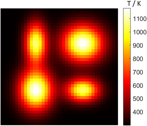
FIGURE 5. The original temperature distribution of the 2D four-peak flame.

Eight linear CCD cameras are arranged on the circle 0.55 m from the flame center. As shown in Figure 6, each camera focuses on the plane passing through the flame center. A lens with a magnification ratio of 1:3 is selected. The number of pixels of each camera is 4,096, and the pixel size is 7.04 µm$\text{μm}$, which ensures that the field of view of each camera covers all the flame domains.

FIGURE 6

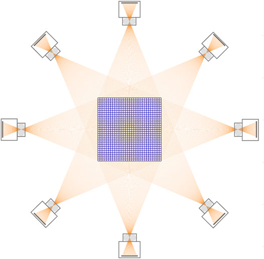
FIGURE 6. The schematic diagram of the layout of the eight linear camera system.

Performance Comparison

According to the arrangement of the camera system and the flame, the flame image of each camera, as shown in Figure 7, is obtained through the calculation of the radiative transfer equation and the reverse tracing of the light. The light that does not pass through any flame voxel is removed to obtain the number of effective rays is 28,304. Thus the scale of the reconstruction coefficient matrix is 28,304 $\times$ 1,600, in which the proportion of non-zero elements to the total elements is 2.46%, the rank of the coefficient matrix is 1,600, and the condition number is 526.13. It can be seen that the reconstruction equations are a typical large-scale sparse ill-conditioned equation system. Since the traditional general solution algorithms do not take into account the characteristics of the reconstruction coefficient matrix, they cannot give full play to their advantages.

FIGURE 7

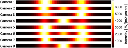
FIGURE 7. The Schematic diagram of the layout of the 8 linear camera system.

The case was implemented using MATLAB code, and the developed program was executed on an Intel(R) Core(TM) i9-10940X CPU @ 3.30 GHz PC. The temperature distribution of the above-mentioned four-peak flame is reconstructed according to the measured flame image using SART, LSQR, NNLS, and Direct Solution algorithm, respectively. The calculation efficiency and accuracy results are shown in Table 1. It can be seen from the table that the reconstruction accuracy of the Direct Solution algorithm is better than the SART and LSQR algorithms and slightly worse than that of the NNLS algorithm in the three reconstruction quality evaluation indicators. This is because the Direct Solution algorithm uses the LSQR algorithm to calculate the small-scale equations, and the NNLS algorithm performs non-negative constraints on the calculation results based on the physical characteristics of the flame so that the method can avoid some local optimal solution that do not conform to the laws of physics.

TABLE 1

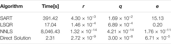
TABLE 1. The comparison of reconstruction performance of different algorithms.

In terms of reconstruction efficiency, the Direct Solution algorithm is 169.4 times higher than the SART algorithm, 7.4 times higher than the LSQR algorithm, and 3483.3 times higher than the NNLS algorithm, which has obvious advantages. This is because the Direct Solution algorithm gradually decomposes the equation system into multiple sub-equation systems and solves them one by one. Each sub-equation system has a few unknowns to solve, avoiding the direct calculation of large-scale equations, which can greatly reduce the calculating time.

Influence of the Grids Number

The size and temperature of the flame area are kept unchanged, and the discrete grids of the flame area is set as 10 × 10, 20 × 20, 40 × 40, and 80 × 80, as shown in Figure 8. In this case, all the camera and lens parameters are kept unchanged. The total number of the detected light is 32,768. After ray tracing, the rays that do not pass through any flame control body are eliminated, and the number of effective rays under the four grids is 28,304.

FIGURE 8

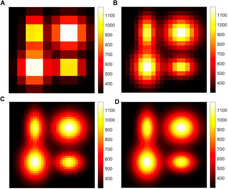
FIGURE 8. The temperature distribution under different grids (A) 10 × 10, (B) 20 × 20, (C) 40 × 40, and (D) 80 × 80.

The flame temperature distribution is reconstructed using the SART algorithm, LSQR algorithm, NNLS algorithm, and Direct Solution algorithm proposed in this paper, and the overall error distribution and calculation time change of the four algorithms under different grids are obtained. The accuracy and efficiency of these algorithms are shown in Figure 9 and Figure 10. It can be seen from the figure that as the number of grids increases, the scale of the equation system expands, and the error presents an upward trend. The reconstruction accuracy of the Direct Solution algorithm is less than that of the NNLS algorithm but better than the SART and LSQR algorithms.

FIGURE 9

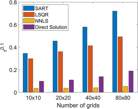
FIGURE 9. The influence of the grids number on the overall reconstruction error.

FIGURE 10

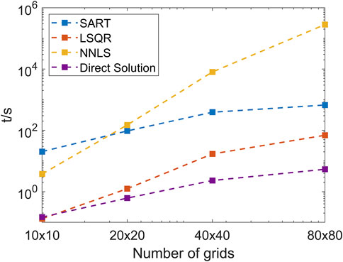
FIGURE 10. The influence of the number of grids on the reconstruction time.

It can be seen from Figure 10 that as the number of grids gradually increases, the calculation time of the four algorithms increases. The calculation time of the Direct Solution algorithm increases slowest, indicating that it is least affected by the increase in the scale of the equations. The direct solution algorithm takes less time than the other three algorithms, indicating that when the number of grids increases, the direct solution algorithm takes less time to extract and solve the partial extraction of the overall equation system. This reduces the overall time-consuming to solve all the unknowns, greatly shortens the reconstruction time compared to other algorithms. The above numerical results show that the Direct Solution algorithm can quickly reconstruct the flame temperature distribution under the premise of ensuring accuracy. In occasions where real-time reconstruction is required, this algorithm has greater application prospects.

Conclusion

In this paper, a Direct Solution algorithm is proposed. It can quickly reconstruct the flame temperature distribution. According to the characteristics of the reconstruction coefficient matrix, it first performs statistical classification according to the minimum non-zero element criterion and the full rank criterion of the sub-equation system. And then, it solves the small-scale equations group by group according to the method of “solving-substitution”, which greatly improves the reconstruction efficiency of large-scale sparse equations. The performance of the proposed method is compared with that of the traditional tomographic reconstruction algorithms. Under the condition of 40 × 40 grids, the normalized average absolute distance criterion r, normalized mean square distance criterion q, and worst-case distance criterion e of the proposed algorithm are all smaller than that of SART and LSQR algorithms. Compared with the SART, LSQR, and NNLS algorithms, the reconstruction efficiency is increased by 169.4, 7.4, and 3483.3 times, respectively. On this basis, the influence of the grids number on the reconstruction algorithm is analyzed. The results show that as the number of grids increases, the reconstruction time of the Direct Solution algorithm increases the slowest. The overall reconstruction accuracy is higher than SART and LSQR methods, which can meet the accuracy requirements on many occasions.

Data Availability Statement

The original contributions presented in the study are included in the article/supplementary material, further inquiries can be directed to the corresponding authors.

Author Contributions

BZ: conceptualization, writing - original draft, and methodology. W-JP: coding and data processing. JL: Investigation and Visualization. Z-HL: writing editing. C-LX: paper reviewing and supervision. All authors contributed to the article and approved the submitted version.

Funding

The supports of this work by the National Natural Science Foundation of China (No. 52176167, 52006036), and the Natural Science Foundation of Jiangsu Province (No. BK20201279, BK20190366) are gratefully acknowledged.

Conflict of Interest

The authors declare that the research was conducted in the absence of any commercial or financial relationships that could be construed as a potential conflict of interest.

Publisher’s Note

All claims expressed in this article are solely those of the authors and do not necessarily represent those of their affiliated organizations, or those of the publisher, the editors and the reviewers. Any product that may be evaluated in this article, or claim that may be made by its manufacturer, is not guaranteed or endorsed by the publisher.

References

Andersen, A. H., and Kak, A. C. (1984). Simultaneous Algebraic Reconstruction Technique (SART): a superior Implementation of the ART Algorithm. Ultrason. Imaging 6 (1), 81–94. doi:10.1016/0161-7346(84)90008-7

PubMed Abstract | CrossRef Full Text | Google Scholar

Bombara, G., Cococcioni, M., Lazzerini, B., and Marcelloni, F. (2011). S-NNLS: An Efficient Non-negative Least Squares Algorithm for Sequential Data. Int. J. Numer. Meth. Biomed. Engng. 27 (5), 770–773. doi:10.1002/cnm.1331

CrossRef Full Text | Google Scholar

Cai, W., Li, X., Li, F., and Ma, L. (20132013). Numerical and Experimental Validation of a Three-Dimensional Combustion Diagnostic Based on Tomographic Chemiluminescence. Opt. Express 21 (6), 7050–7064. doi:10.1364/OE.21.007050

PubMed Abstract | CrossRef Full Text | Google Scholar

Gamil, A. A. A., Nikolaidis, T., Lelaj, I., and Laskaridis, P. (2020). Assessment of Numerical Radiation Models on the Heat Transfer of an Aero-Engine Combustion Chamber. Case Stud. Therm. Eng. 22, 100772. doi:10.1016/j.csite.2020.100772

CrossRef Full Text | Google Scholar

He, L., Chen, Y., Deng, J., Lei, J., Fei, L., and Liu, P. (2019). Experimental Study of Rotating Gliding Arc Discharge Plasma-Assisted Combustion in an Aero-Engine Combustion Chamber. Chin. J. Aeronautics 32 (2), 337–346. doi:10.1016/j.cja.2018.12.014

CrossRef Full Text | Google Scholar

Hossain, M. M., Lu, G., Sun, D., and Yan, Y. (2013). Three-dimensional Reconstruction of Flame Temperature and Emissivity Distribution Using Optical Tomographic and Two-Colour Pyrometric Techniques. Meas. Sci. Technol. 24 (7), 074010. doi:10.1088/0957-0233/24/7/074010

CrossRef Full Text | Google Scholar

Huang, X., Qi, H., Zhang, X.-L., Ren, Y.-T., Ruan, L.-M., and Tan, H.-P. (2018). Application of Landweber Method for Three-Dimensional Temperature Field Reconstruction Based on the Light-Field Imaging Technique. J. Heat Trans. –T. ASME 140, 082701–082711. doi:10.1115/1.4039305

CrossRef Full Text | Google Scholar

Jenkins, T. P., Hess, C. F., Allison, S. W., and Eldridge, J. I. (2020). Measurements of Turbine Blade Temperature in an Operating Aero Engine Using Thermographic Phosphors. Meas. Sci. Technol. 31 (4), 044003. doi:10.1088/1361-6501/ab4c20

CrossRef Full Text | Google Scholar

Li, J., Hossain, M. M., Sun, J., Liu, Y., Zhang, B., Tachtatzis, C., et al. (2019). Simultaneous Measurement of Flame Temperature and Absorption Coefficient through LMBC-NNLS and Plenoptic Imaging Techniques. Appl. Therm. Eng. 154, 711–725. doi:10.1016/j.applthermaleng.2019.03.130

CrossRef Full Text | Google Scholar

Li, L., Peng, X. F., and Liu, T. (2006). Combustion and Cooling Performance in an Aero-Engine Annular Combustor. Appl. Therm. Eng. 26 (16), 1771–1779. doi:10.1016/j.applthermaleng.2005.11.023

CrossRef Full Text | Google Scholar

Lian, W., and Xuan, Y. (2017). Experimental Investigation on a Novel Aero-Engine Nose Cone Anti-icing System. Appl. Therm. Eng. 121, 1011–1021. doi:10.1016/j.applthermaleng.2017.04.160

CrossRef Full Text | Google Scholar

Liu, D., Yan, J. H., Wang, F., Huang, Q. X., Chi, Y., and Cen, K. F. (2010). Inverse Radiation Analysis of Simultaneous Estimation of Temperature Field and Radiative Properties in a Two-Dimensional Participating Medium. Int. J. Heat Mass Transfer 53 (21-22), 4474–4481. doi:10.1016/j.ijheatmasstransfer.2010.06.046

CrossRef Full Text | Google Scholar

Liu, S., Liu, S., and Ren, T. (2017). Acoustic Tomography Reconstruction Method for the Temperature Distribution Measurement. IEEE Trans. Instrum. Meas. 66 (8), 1936–1945. doi:10.1109/TIM.2017.2677638

CrossRef Full Text | Google Scholar

Marahleh, G., Kheder, A. R. I., and Hamad, H. F. (2006). Creep-life Prediction of Service-Exposed Turbine Blades. Mater. Sci. 42 (4), 476–481. doi:10.1007/s11003-006-0103-8

CrossRef Full Text | Google Scholar

Neuer, G., Fischer, J., Edler, F., and Thomas, R. (2001). Comparison of Temperature Measurement by Noise Thermometry and Radiation Thermometry. Measurement 30 (3), 211–221. doi:10.1016/S0263-2241(01)00006-9

CrossRef Full Text | Google Scholar

Niu, C.-Y., Qi, H., Huang, X., RuanRuan, L.-M. L. M., Wang, W., and Tan, H.-P. (2015). Simultaneous Reconstruction of Temperature Distribution and Radiative Properties in Participating media Using a Hybrid LSQR-PSO Algorithm. Chin. Phys. B 24 (11), 114401. doi:10.1088/1674-1056/24/11/114401

CrossRef Full Text | Google Scholar

Qi, H., Niu, C.-Y., Gong, S., Ren, Y.-T., and Ruan, L.-M. (2015). Application of the Hybrid Particle Swarm Optimization Algorithms for Simultaneous Estimation of Multi-Parameters in a Transient Conduction-Radiation Problem. Int. J. Heat Mass Transfer 83, 428–440. doi:10.1016/j.ijheatmasstransfer.2014.12.022

CrossRef Full Text | Google Scholar

Qi, Q., Hossain, M. M., Zhang, B., Ling, T., and Xu, C. (2019). Flame Temperature Reconstruction through a Multi-Plenoptic Camera Technique. Meas. Sci. Technol. 30 (12), 124002. doi:10.1088/1361-6501/ab2e98

CrossRef Full Text | Google Scholar

Qiu, S., Lou, C., and Xu, D. (2014). A Hybrid Method for Reconstructing Temperature Distributions in a Radiant Enclosure. Numer. Heat Transfer, A: Appl. 66 (10), 1097–1111. doi:10.1080/10407782.2014.901034

CrossRef Full Text | Google Scholar

Resnick, J. (1985). The Radon Transforms and Some of its Applications. IEEE Trans. Acoust. Speech, Signal. Process. 33 (1), 338–339. doi:10.1109/TASSP.1985.1164533

CrossRef Full Text | Google Scholar

Sun, J., Hossain, M. M., Xu, C., and Zhang, B. (2018). Investigation of Flame Radiation Sampling and Temperature Measurement through Light Field Camera. Int. J. Heat Mass Transfer 121, 1281–1296. doi:10.1016/j.ijheatmasstransfer.2018.01.083

CrossRef Full Text | Google Scholar

Teng, K. F., and Ping Wu, P. (1989). PV Module Characterization Using Q-R Decomposition Based on the Least Square Method. IEEE Trans. Ind. Electron. 36 (1), 71–75. doi:10.1109/41.20347

CrossRef Full Text | Google Scholar

Yang, L., and Zhi-min, L. (2015). The Research of Temperature Indicating Paints and its Application in Aero-Engine Temperature Measurement. Proced. Eng. 99, 1152–1157. doi:10.1016/j.proeng.2014.12.697

CrossRef Full Text | Google Scholar

Zhang, B., Xu, C.-L., and Wang, S.-M. (2017). Generalized Source Finite Volume Method for Radiative Transfer Equation in Participating media. J. Quantitative Spectrosc. Radiative Transfer 189, 189–197. doi:10.1016/j.jqsrt.2016.11.025

CrossRef Full Text | Google Scholar

Zhang, B., Xu, C. L., and Wang, S. M. (2016). An Inverse Method for Flue Gas Shielded Metal Surface Temperature Measurement Based on Infrared Radiation. Meas. Sci. Technol. 27 (7), 074002. doi:10.1088/0957-0233/27/7/074002

CrossRef Full Text | Google Scholar

Zhang, R. C., Huang, X. Y., Fan, W. J., and Bai, N. J. (2019). Influence of Injection Mode on the Combustion Characteristics of Slight Temperature Rise Combustion in Gas Turbine Combustor with Cavity. Energy 179 (15), 603–617. doi:10.1016/j.energy.2019.04.223

CrossRef Full Text | Google Scholar

Zhao, W., Zhang, B., Xu, C., Duan, L., and Wang, S. (2018). Optical Sectioning Tomographic Reconstruction of Three-Dimensional Flame Temperature Distribution Using Single Light Field Camera. IEEE Sensors J. 18 (2), 528–539. doi:10.1109/JSEN.2017.2772899

CrossRef Full Text | Google Scholar

Zhou, H.-C., Han, S.-D., Sheng, F., and Zheng, C.-G. (2002). Visualization of Three-Dimensional Temperature Distributions in a Large-Scale Furnace via Regularized Reconstruction from Radiative Energy Images: Numerical Studies. J. Quantitative Spectrosc. Radiative Transfer 72 (4), 361–383. doi:10.1016/S0022-4073(01)00130-3

CrossRef Full Text | Google Scholar