A mixed integer linear programming model for minimum backbone grid

1 Introduction

In recent years, as the global climate continues to warm, extreme weather occurs frequently, which seriously affects the reliability of power supply and the national economy. In the power system planning, a minimum backbone grid can be developed. The selected generators and lines in the minimum backbone grid can be reinforced before the extreme weather to ensure the supply of critical loads in extreme weather. After the extreme weather, the power system can be quickly restored to the normal state by the stable power supply of the grid. In summary, developing a minimum backbone grid is beneficial to ensure the uninterrupted power supply of important loads and rapid recovery of core power infrastructure under extreme disaster conditions. It improves the ability of the power grid to respond to low-probability extreme events, which is an important part of resilience in the power grid (Mahzarnia et al., 2020; Trudel et al., 2005; Bie et al., 2017). How to develop a minimum backbone grid from the existing power grid is the core of the research.

At present, the research on developing a minimum backbone grid can be divided into two categories:

One is the heuristic method. The method has been widely used in developing a minimum backbone grid because it is not limited by the non-convexity and non-smoothness of the optimization problem and can quickly obtain a feasible solution. In Yang et al. (2010), a minimum grid model considering the importance of lines and the topology of the grid is constructed, and binary particle swarm optimization is used to solve the model. In Liu et al. (2007), the topological characteristics of scale-free networks are employed to obtain a skeleton-network reconfiguration strategy, and the discrete particle swarm optimization technique is employed to implement the reconfiguration. Rather than providing a detailed restoration path sequence, the strategy aims to obtain several better-performing reconfiguration schemes as the guidance of dispatching operations. In Dong et al. (2015), the authors present a comprehensive index system to measure the survivability of the backbone grid and a new method of constructing the grid considering survivability. The improved biogeographic optimization algorithm provided with strong search ability is used to obtain the optimal solution for the core backbone grid. In Chen, (2021), a risk assessment system of power grid operation involving multi-link uncertain factors is proposed, and a core backbone grid model considering the minimum comprehensive risk index is constructed. The traditional fireworks algorithm is improved to quickly and accurately search the construction scheme of the optimal backbone grid. The above heuristic algorithm is simple and easy to use, compared with the general mathematical programming method. However, it is poor robust and its result is random, which makes it difficult to reproduce and repeatedly check the results in practical applications (Blum and Roli, 2003; Ball, 2011).

The other is the mathematical programming method, which is rarely studied in this research. In Sun et al. (2019), aiming at maximum network restoration efficiency, the optimal backbone grid is formulated as a MILP problem, which can be efficiently solved by commercial solvers such as CPLEX. However, the model cannot ensure the connectivity of the minimum backbone grid, which makes the grid likely to have islands. Then, the backbone grid will be of low reliability, which is not conducive to the survival and rapid recovery of the grid under extreme disaster conditions. Network connectivity is a major bottleneck in the application of mathematical programming methods to this problem. Table 1 compares the method, objective and connectivity method between the existing literature.

TABLE 1

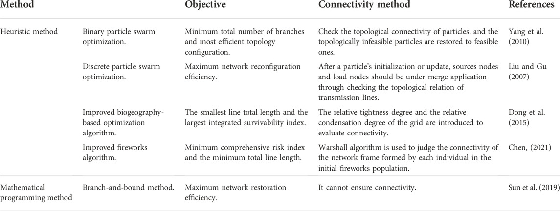
TABLE 1. Minimum backbone grid problems compared with selected references.

In this paper, we also present a mathematical programming method in which a mixed integer linear programming model for a minimum backbone grid is proposed. A minimum number of branches and maximum summation of power flow betweenness objective function is considered in the model. Furthermore, a set of close-form connectivity constraints is formulated to ensure the reliability of the backbone grid. The main contributions of this paper are as follows:

• The minimum backbone grid is described as a MILP model. It considers constraints presented to the practical application requirements such as regional plant constraints.

• Based on the idea of single commodity flow, it considers a set of linear constraints on the grid connectivity, which avoids the island of minimum backbone grid, overcomes the defect that the existing methods are difficult to express the connectivity constraints rigorously, and breaks through the bottleneck of mathematical programming method in the application of this problem.

The simulation results of the IEEE-39 bus system and the French 1888 bus system verify the effectiveness of the proposed model and show that the proposed method has high computational efficiency.

2 Construction planning of minimum backbone grid

The minimum backbone grid is a minimum grid that can ensure the continuous power supply of important loads. The goal is to minimize the scale of the grid, that is, to minimize the number of branches. The backbone grid must satisfy specific constraints such as power balance constraints, line capacity constraints, connectivity constraints, and so on to ensure that it operates under special circumstances. In order to describe the backbone grid quantitatively, some specific constraints to the backbone grid are given as follows:

1) Satisfying the security operation constraints of the power grid;

2) Satisfying the connectivity of network topology;

3) Maintaining specific system load level;

4) Guarantee regional power sources;

5) On basis of satisfying the above constraints, the number of branches in the backbone grid should be the minimum;

The backbone grid also needs to obey special requirements for different situations. This paper gives basic definitions and models that can be expanded on this basis in various situations.

Developing a minimum backbone grid involves determining the critical loads, and selecting essential generators and backbone lines.

2.1 Determining critical loads

The critical loads include the urban emergency dispatch center, core infrastructures such as communication, water supply, and transportation, large densely residential areas, and important customers. Since most critical loads are distributed in the distribution network at a low voltage level, it is necessary to progressively search the corresponding load buses in transmission substations from low voltage to high voltage levels. The range and quantity of the critical loads directly affect the scale of the minimum backbone grid. Excessive critical loads will make the minimum backbone grid too large, resulting in a high investment. Therefore, the proportion of the critical loads should not be too high.

2.2 Selecting essential generators

Selecting essential generators follows the general principles:

1) Trying to ensure each region of the power grid has generators to avoid the blackout in case of regional tie line failure.

2) Preferring to choose the hydro generators in the backbone grid, as the hydro generators have the advantages of simple auxiliary equipment and rapid startup (Adibi and Fink, 2006).

3) The priority of synchronous generators connected to the power grid through a lower voltage level should be higher than that of synchronous generators connected to the power grid through a higher voltage level to ensure that the power locally supplies the backbone load.

2.3 Selecting backbone lines

The principle of backbone line selection is as follows:

1) The two adjacent higher voltage level substations selected into the minimum backbone grid should be connected by lower voltage level lines to strengthen the support between critical areas.

2) According to the characteristics of natural disasters in various regions, some backbone lines should have higher priority. For example, typhoons in some areas generally travel from east to west. In this case, the east-west lines should be preferred in the minimum backbone grid. In the ice disaster scenario, the lines with ice melting devices should be selected as a high priority.

3 Mathematical programming model of minimum backbone grid

3.1 Basic mathematical model

3.1.1 Objective function

The objective function considers two aspects, one is to ensure as few branches as possible, and the other is to preferentially select branches with high importance. The power flow betweenness (Rout et al., 2016) is used as an index to measure the importance of branches.

The objective function is as follows:

$\min {\displaystyle \sum }_{\left(i,j\right)\in L}\left(w+\left(1-F_{ij}\right)\right)s_{ij}(1)$

where $L$ is the set of branches of the power grid, $s_{ij}$ is the state of the branch, take 1 as the line is included in the minimal backbone grid, otherwise take 0, $w$ is a constant greater than 1, the purpose is to make the objective function focus more on the minimum number of branches than the maximum importance of branches, $F_{ij}$ is the normalized power flow betweenness of the branch $i-j$. To preferentially select the lower voltage level synchronous generators or certain lines, the power flow betweenness of related lines can be increased.

3.1.2 Constraints

1) Active power balance constraints:

$\begin{array}{cc}{\displaystyle \sum }_{g\in G_i}{p}_g-{\displaystyle \sum }_{\left(i,j\right)\in L_i}{p}_{ij}={\displaystyle \sum }_{d\in D_i}{p}_d,& i\in B\end{array}(2)$

where $G_i$ is the generator set on the bus $i$, $p_g$ is the active output of the generator$g$, $L_i$ is the line set with $i$ as the starting bus, $p_{ij}$ is the active power of line$i-j$, $D_i$is the critical load set at bus $i$; $p_d$ is the active power of load $d$, $B$ is the bus set.

2) Generator operating constraints:

$\begin{array}{cc}{u}_g{p}_g^{\min }\le p_g\le u_g{p}_g^{\max },& g\in G\end{array}(3)$

where $p_g^{\min }$ and $p_g^{\max }$ are the minimum and maximum active power of generator$g$, $u_g$is unit status, take 1 if unit $g$ is included in the minimum backbone grid, otherwise, take 0.

3) Line capacity constraints:

$\begin{array}{cc}-p_{ij}^{\max }{s}_{ij}\le p_{ij}\le p_{ij}^{\max }{s}_{ij},& \left(i,j\right)\in L\end{array}(4)$

where $p_{ij}^{\max }$ is the rated capacity of line $i-j$.

4) DC power flow constraints:

$\begin{array}{cc}\left(s_{ij}-1\right)M_{ij}\le p_{ij}+B_{ij}{\theta }_{ij}\le \left(1-s_{ij}\right)M_{ij},& \left(i,j\right)\in L\end{array}(5)$

where $M_{ij}$ is a large constant for line$i-j$, ${\theta }_{ij}$ and $B_{ij}$ are the phase angle difference between bus $i$and $j$, the imaginary part of line $i-j$ admittance.

5) Phase angle constraint:

${\theta }_{slack}=0(6)$

$-M_{ij}\left(1-s_{ij}\right)+{\underset{¯}{\theta }}_{ij}\le {\theta }_{ij}\le M_{ij}\left(1-s_{ij}\right)+{\overline{\theta }}_{ij},\left(i,j\right)\in L(7)$

where ${\theta }_{slack}$ is the phase-angle of the balance bus, ${\underset{¯}{\theta }}_{ij}$ and ${\overline{\theta }}_{ij}$ are the minimum and maximum of ${\theta }_{ij}$.

6) Regional plant constraints:

According to the selection principle of generators, each area has at least one generator, that is

$\begin{array}{cc}{\displaystyle \sum }_{g\in G_a}{u}_g>0,& a\in A\end{array}(8)$

where $G_a$ is the generator set of area $a$, $A$is the set of all areas of the whole power grid.

7) Spinning reserve constraint:

${\displaystyle \sum }_{g\in G}\left(u_g{p}_g^{\max }-u_g{p}_g\right)\ge SR(9)$

where $G$ is the set of all generators, $SR$ is the minimum spinning reserve required by the system.

8) Primary frequency reserve constraint:

${\displaystyle \sum }_{g\in G}{\beta }_g{u}_g{p}_g^{\max }\ge \mathit{PR}(10)$

where ${\beta }_g$ is the primary frequency regulation coefficient of generator $g$, generally 15% for hydro generator units and 5% for thermal generators (Adibi and Fink, 2006), $\mathit{PR}$ is the minimum primary frequency reserve required by the system. This constraint can make the minimum backbone grid model give priority to select hydro generators.

9) Must-in-service line constraints:

$\begin{array}{cc}{s}_{ij}=1,& \left(i,j\right)\in L_{in}\end{array}(11)$

where $L_{in}$ is the set of must-in-service lines. Some lines with a high strength level or lines with ice melting devices in ice disaster protection scenarios must be included in the minimum backbone grid and can be set as must-in-service lines.

10) Must-out line constraints:

$\begin{array}{cc}{s}_{ij}=0,& \left(i,j\right)\in L_{ex}\end{array}(12)$

where $L_{ex}$ is the set of must-out lines. Lines with a low strength level should not be included in the minimum backbone grid and can be set as must-out lines.

11) Must-on generator constraints:

$\begin{array}{cc}{u}_g=1,& g\in G_{in}\end{array}(13)$

where $G_{in}$ is the set of must-on generators. Some black-start generators are always set to be must-on generators.

3.2 Connectivity constraints

In the minimum backbone grid model, the connectivity constraint is an important constraint to ensure the reliability and recovery ability of the grid. However, the existing research lacks methods of expressing network connectivity. Network connectivity constraints are widely used in traveling salesman problems, vehicle routing problems, minimum spanning tree problems, and Steiner tree problems (Gollowitzer and Ljubic., 2011). In these problems, single-commodity flow is commonly used to formulate connectivity constraints.

The idea of the single commodity flow constraint is to set the node that sends out the commodity as the root point and the node that requires the commodity as the sink point in a directed graph$\left(V,A\right)$. Through constraint (14), each sink point can receive the required commodity from the root point, which ensures the connectivity between the root point and each sink point, thus ensuring the connectivity of the network.

${\displaystyle \sum }_{ji\in L_s}{f}_{ji}-{\displaystyle \sum }_{ij\in L_s}{f}_{ij}=\{\begin{array}{l}1i\in K,\\ -\left|K\right|i=r,\\ 0\left(\frac{i\in V}{\left\{K,r\right\}}\right),\end{array}(14)$

where $V$ is the set of all nodes, $L_s$ is the set of all directed branches, $r$ is a root point, $\left|K\right|$ is the number of nodes in the sink set $K$, and $f_{ij}$ is the virtual flow from node $i$ to node $j$ through the line$i-j$.

At the same time, constraint (15) can ensure that the amount of virtual flow passed by each branch does not exceed the actual line capacity.

$0\le f_{ij}\le \left|K\right|x_{ij}(15)$

where $x_{ij}$ is the state of the directed branch, take 1 if it is included in the connectivity network, otherwise take 0.

In the minimum backbone grid, a must-on generator in the power grid can be selected as the root point. $L_s$contains all branches of the power grid in two power flow directions. Thus, the number of elements in the set is twice the number of actual branches. There is also the following relationship between $s_{ij}$ and $x_{ij}$ in the minimum backbone grid:

$\begin{array}{cc}{s}_{ij}=x_{ij}+x_{ji},& (i,j\end{array})\in L(16)$

3.3 Implementation process of minimum backbone grid

The steps of obtaining a minimum backbone grid are as follows:

1) Input the parameters of the original grid, including line and transformer data, etc.

2) Calculate the normalized power flow betweenness of all branches.

3) Determine object constant, critical loads level, must-on generators, must-in and must-out lines and system reserve.

4) Solve the minimum backbone grid model in Section 3.

5) If the backbone grid is not small enough, increase the object constant or decrease the critical loads level and go to step 3.

The implementation flowchart of the minimum backbone grid is shown in Figure 1:

FIGURE 1

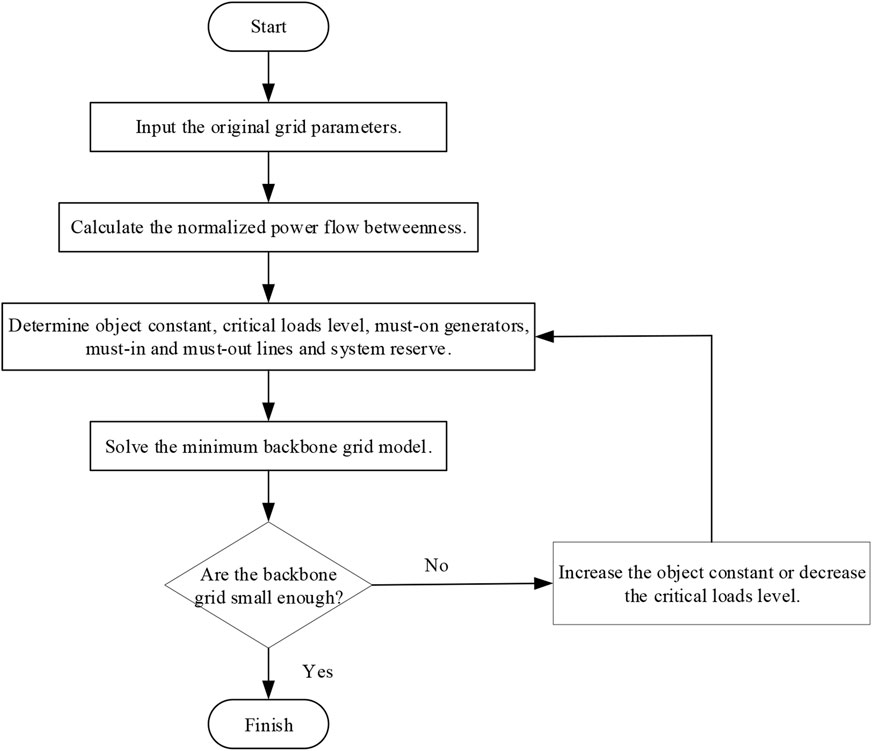
FIGURE 1. Implementation flowchart of minimum backbone grid.

4 Case studies

To verify the validity of the proposed model, the IEEE-39 bus system (Yeu, 2010) and the French 1888 bus system (Zimmerman et al., 2011) are simulated. All simulations are implemented on a PC with a Core i7 2.9-GHz CPU and 16.0 GB RAM, using mathematical modeling software Pyomo 6.2 and Gurobi 9.5.1 solver to solve the established optimization model, and the convergence gap is set to 0.0001.

4.1 IEEE-39 bus system

Table 2 shows the normalized power flow betweenness of each line of the IEEE-39 bus system, and Table 3 shows the critical loads in the minimum backbone grid. Due to the small size of the IEEE-39 bus system, regional plant constraints were not considered.

TABLE 2

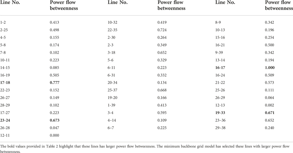
TABLE 2. Flow betweenness of lines in IEEE 39-bus system.

TABLE 3

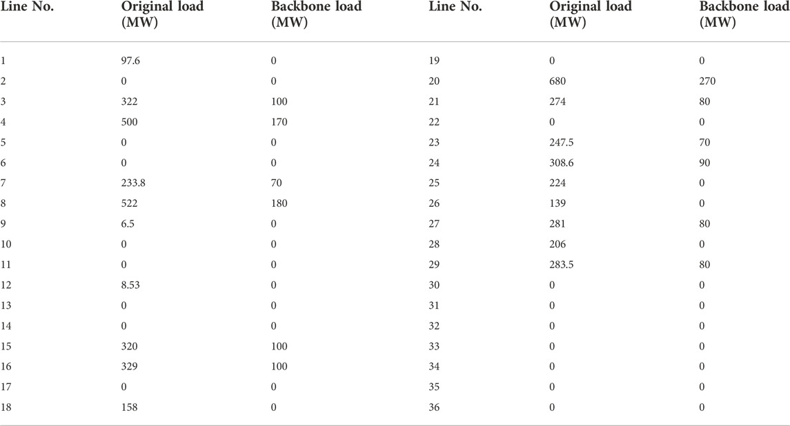
TABLE 3. The critical load setting in backbone grid of IEEE 39-bus system.

After the calculation, the minimum backbone grid is shown in Figure 2 in red color. Figure 2 shows the grid has 24 lines, 3 generators, which is only 52.17% of the original grid, and all the critical loads in Table 2. Especially, the backbone grid is connected. Reinforcing the 52.17% can ensure the power supply for critical loads of the whole grid under extreme weather. To transmit power to node 29, there are two paths between node 26 and node 29, one is 26-29, and the other is 26-28, 28-29. Line 26-29 is selected by the minimum backbone grid model as expected due to the objective function, that is, the number of lines will be selected as few as possible. In addition, the model has selected lines with larger power flow betweenness, such as lines 16-17, 17-18, 23-24, and 19-33. Other lines with larger power flow betweenness, such as lines 22-35, 25-37, and 23-36, have not been selected because they are outlet lines of unpowered generators. Thus, it can be seen that the objective function is effective and correct.

FIGURE 2

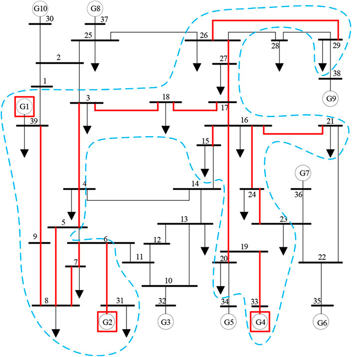
FIGURE 2. IEEE 39-bus system backbone grid considering connectivity constraints.

We also compared our proposed MILP method with four heuristic methods. Due to the random results of the heuristic methods, the results listed in Table 4 are obtained based on 100 times running.

TABLE 4

TABLE 4. Comparison with the heuristic methods for IEEE 39-bus system.

From the Table 4, it can be seen that the MILP method has the same lines in minimum backbone grid for every running. By contrast, the heuristic methods have different lines in minimum backbone grid for different running. Furthermore, the MILP method gets the optimal lines which is less than the best value of the heuristic methods in minimum backbone grid.

After removing connectivity constraints (14–18) and retaining other constraints, recalculate the model and the result is shown in Figure 3. There are 18 lines and six generators in the figure. Although the number of lines in this minimum backbone grid is less than that in Figure 2, the minimum backbone grid is not connected and there are five islands. Each island has generator nodes and load nodes to meet power balance. However, the recoverability and reliability of the unconnected grid are low. These five islands are very fragile and very hard to keep frequency or rotor angle stability. They may be blackout following a further disturbance. Once the island is blackout, it will need more time to restore the power grid. This demonstrates the validity of the connectivity constraints proposed in this paper.

FIGURE 3

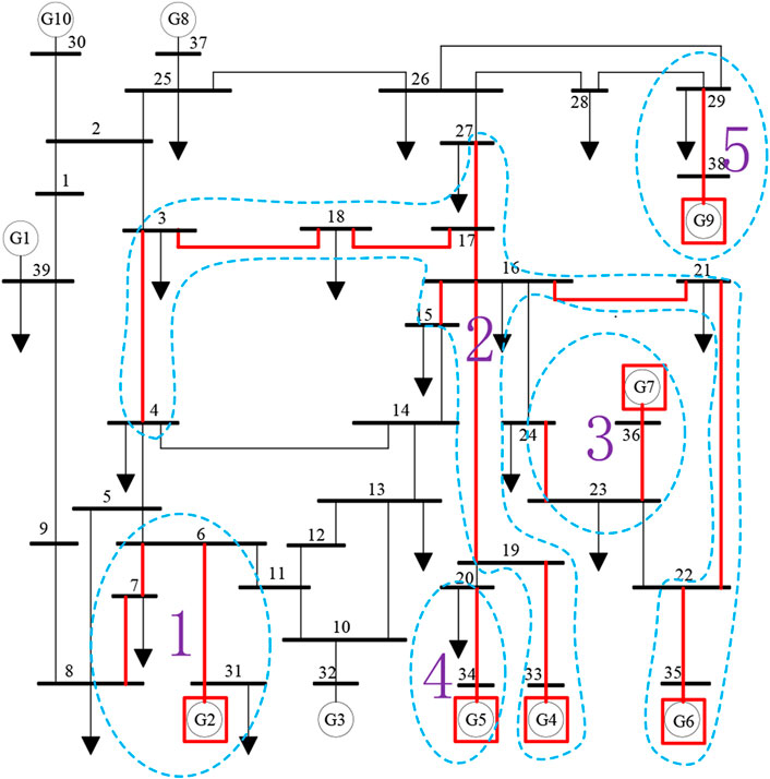
FIGURE 3. IEEE 39-bus system backbone grid without connectivity constraints.

4.2 French 1888 bus system

The French 1888 bus system is from the data file (CASE1888RTE) in matpower7.0 and has 2,531 branches. To facilitate the test, the backbone load is set as 15% of the original load. The objective function of the minimum backbone grid model involves two objectives, the minimum number of branches and the maximum summation of power flow betweenness. The purpose of setting $w$ is that the objective of minimizing the number of branches in the minimum backbone grid should take precedence over the objective of maximizing the summation of power flow betweenness. Different weights$w$are set to calculate the model, and the number of lines and the summation of power flow betweenness of the minimum backbone grid are shown in Table 5.

TABLE 5

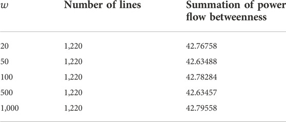
TABLE 5. Number of branches and summation of branch betweenness for backbone grid of the French 1888 bus system with different $w$

As can be seen from Table 5, with the increase of $w$, the number of lines in the grid does not change, and the summation of the power flow betweenness varies slightly but all within the acceptable range. This shows that the goal of the minimum number of branches has been given priority, and it is not greatly affected by $w$. This feature makes the user less demanding to set weights $w$ and makes the method robust.

Table 6 shows the number of constraints and calculation time of the model with and without connectivity constraints. Although considering the connectivity constraints will increase the size of the model, the calculation time is shorter than that of the model without the connectivity constraints. This is because the connectivity constraints tighten the feasible region of MILP, and the algorithm of MILP is easier to find the optimal solution. In addition, for such a large-scale system, the solution can be obtained in an acceptable time, which shows that the mathematical programming method is very efficient.

TABLE 6

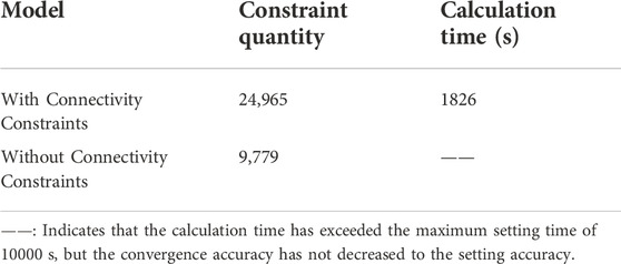
TABLE 6. Number of constraints and computing time for the model with and without connectivity constraints.

Of course, there are some methods to further improve the calculation efficiency of the model, such as further tightening the model according to its characteristics of the model or tuning the parameters of the solver.

5 Conclusion

A mixed integer linear programming model for a minimum backbone grid is proposed in this paper, which considers the practical application requirements. More importantly, the model can ensure network connectivity to avoid islands in the grid, which is an important prerequisite for the practical application of mathematical programming methods in developing a minimum backbone grid. The simulations on the IEEE-39 bus system and the French 1888 bus system verify the validity of the proposed model and show that the minimum backbone grid has a small scale of only 52% of the original grid and the proposed method has high computational efficiency of only about 30 min for such a large system.

Data availability statement

The original contributions presented in the study are included in the article/Supplementary Material, further inquiries can be directed to the corresponding author.

Author contributions

Conceptualization, WM and PL; methodology, WM and PL; software, WM and YH; validation, WM and ZS; resources, WM; data curation, WM and PL; writing—original draft preparation, WM; writing—review and editing, WM, ML, XG, and PL; super-vision, PL. All authors have read and agreed to the published version of the manuscript.

Funding

This research was supported in part by the National Natural Science Foundation of China under Grant no. 51967001, 51967002 and 52267006, in part by Guangxi Special Fund for Innovation-Driven Development under Grant no.AA19254034, and in part by Guangxi Key Laboratory of Power System Optimization and Energy Technology Research Grant.

Conflict of interest

Authors ZS and ML were employed by the company Guangxi Power Grid Co., Ltd., YH was employed by the company Power China Engineering Co., Ltd., and XG was employed by the company Guangdong Power Grid Co., Ltd.

The remaining authors declare that the research was conducted in the absence of any commercial or financial relationships that could be construed as a potential conflict of interest.

Publisher’s note

All claims expressed in this article are solely those of the authors and do not necessarily represent those of their affiliated organizations, or those of the publisher, the editors and the reviewers. Any product that may be evaluated in this article, or claim that may be made by its manufacturer, is not guaranteed or endorsed by the publisher.

References

Adibi, M. M., and Fink, L. H. (2006). Overcoming restoration challenges associated with major power system disturbances - restoration from cascading failures. IEEE Power Energy Mag. 4, 68–77. doi:10.1109/mpae.2006.1687819

CrossRef Full Text | Google Scholar

Ball, M. O. (2011). Heuristics based on mathematical programming. Surv. Operations Res. Manag. Sci. 16, 21–38. doi:10.1016/j.sorms.2010.07.001

CrossRef Full Text | Google Scholar

Bie, Z., Lin, Y., Li, G., and Li, F. (2017). Battling the extreme: A study on the power system resilience. Proc. IEEE 105, 1253–1266. doi:10.1109/jproc.2017.2679040

CrossRef Full Text | Google Scholar

Blum, C., and Roli, A. (2003). Metaheuristics in combinatorial optimization: Overview and conceptual comparison. ACM Comput. Surv. 35, 268–308. doi:10.1145/937503.937505

CrossRef Full Text | Google Scholar

Chen, Y. (2021). “Construction method of core backbone grid based on improved fireworks algorithm and risk theory,” in 2021 international conference on advanced Technology of electrical engineering and Energy (ATEEE), 62–68.

CrossRef Full Text | Google Scholar

Dong, F., Liu, D., Wu, J., Ke, L., Song, C., Wang, H., et al. (2015). Constructing core backbone network based on survivability of power grid. Int. J. Electr. Power & Energy Syst. 67, 161–167. doi:10.1016/j.ijepes.2014.10.056

CrossRef Full Text | Google Scholar

Gollowitzer, S., and Ljubic, I. (2011). MIP models for connected facility location: A theoretical and computational study. Comput. Operations Res. 38, 435–449. doi:10.1016/j.cor.2010.07.002

PubMed Abstract | CrossRef Full Text | Google Scholar

Heidari, A. A., Mirjalili, S., Faris, H., Aljarah, I., Mafarja, M., and Chen, H. (2019). Harris hawks optimization: Algorithm and applications. Future Gener. Comput. Syst. 97, 849–872. doi:10.1016/j.future.2019.02.028

CrossRef Full Text | Google Scholar

Liu, Y., and Gu, X. (2007). Skeleton-network reconfiguration based on topological characteristics of scale-free networks and discrete particle swarm optimization. IEEE Trans. Power Syst. 22, 1267–1274. doi:10.1109/tpwrs.2007.901486

CrossRef Full Text | Google Scholar

Mahzarnia, M., Moghaddam, M. P., Baboli, P. T., and Siano, P. (2020). A review of the measures to enhance power systems resilience. IEEE Syst. J. 14, 4059–4070. doi:10.1109/jsyst.2020.2965993

CrossRef Full Text | Google Scholar

Mirjalili, S., and Lewis, A., (2016). The whale optimization algorithm. Adv. Eng. Softw. 95, 51–67. doi:10.1016/j.advengsoft.2016.01.008

CrossRef Full Text | Google Scholar

Mirjalili, S., Mirjalili, S. M., and Lewis, A. (2014). Grey wolf optimizer. Adv. Eng. Softw. 69, 46–61. doi:10.1016/j.advengsoft.2013.12.007

CrossRef Full Text | Google Scholar

Rao, R. V., Savsani, V. J., and Vakharia, D. P. (2012). Teaching–Learning-Based Optimization: An optimization method for continuous non-linear large scale problems. Inf. Sci. 183, 1–15. doi:10.1016/j.ins.2011.08.006

CrossRef Full Text | Google Scholar

Rout, G. K., Chowdhury, T., and Chanda, C. K. (2016). Betweenness as a tool of vulnerability analysis of power system. J. Inst. Eng. India. Ser. B 97, 463–468. doi:10.1007/s40031-016-0222-z

CrossRef Full Text | Google Scholar

Sun, L., Lin, Z., Xu, Y., Wen, F., Zhang, C., and Xue, Y. (2019). Optimal skeleton-network restoration considering generator start-up sequence and load pickup. IEEE Trans. Smart Grid 10, 3174–3185. doi:10.1109/tsg.2018.2820012

CrossRef Full Text | Google Scholar

Trudel, G., Gingras, J. P., and Pierre, J. R. (2005). Designing a reliable power system: Hydro-quebec's integrated approach. Proc. IEEE 93, 907–917. doi:10.1109/jproc.2005.846332

CrossRef Full Text | Google Scholar

Yang, W. H., Bi, T. S., Huang, S. F., Xue, A. C., and Yang, Q. X. (2010). “Identification of backbone-grid in power grid based on binary particle swarm optimization,” in 2010 international conference on power system Technology, 1–6.

CrossRef Full Text | Google Scholar

Yeu, R. H. (2010). Small signal analysis of power systems: Eigenvalue tracking method and eigenvalue estimation contingency screening for DSA. Urbana Champagne, IL: University of Illinois at Urbana-Champaign.

Google Scholar

Zimmerman, R. D., Murillo-Sanchez, C. E., and Thomas, R. J. (2011). Matpower: Steady-state operations, planning and analysis tools for power systems research and education. IEEE Trans. Power Syst. 26, 12–19. doi:10.1109/tpwrs.2010.2051168

CrossRef Full Text | Google Scholar