Robust dispatching model of active distribution network considering PV time-varying spatial correlation

1 Introduction

As a clean and sustainable renewable energy source, photovoltaic (PV) generation has become one of the world’s fastest-growing energy sources, progressively becoming the primary source of electricity in power system (Calcabrini et al., 2019). However, owing to the correlation and uncertainty of PV output, the high proportion of PV in the active distribution network (ADN) significantly influences ADN operation and increases the complexity of dispatching (Yu et al., 2015; Haque and Wolfs, 2016). Thus, a reasonable consideration of the correlation and uncertainty of PV outputs in the ADN dispatching model can help enhance PV consumption and promote the balanced development of the ADN.

First, the modeling of PV-output spatial correlation is considered. According to earlier research, there is a spatial correlation between the PV output attributed to locational considerations, micrometeorological circumstances (Ding and Mather, 2017). Currently, common methods to establish a PV-output spatial-correlation model mainly include correlation coefficient matrices, covariance matrix, Copula function, and deep neural network. In (Wu et al., 2021), the Pearson correlation coefficient matrix was used to calculate the spatial correlation of the two PVs, from which empirical distributions of spatial correlation coefficients and distances were obtained. In (Luo et al., 2020), the Kendall rank correlation coefficient, which can measure the correlation of nonlinear variables, was used as the parameter of the Frank-Copula function. Various correlation coefficient matrices were used to evaluate and compare the numerical values of PV-output spatial correlation. In (Wu et al., 2022), a covariance-based spatiotemporal correlation model was proposed to quantify and exploit the PV output spatial correlation. In (Pan et al., 2019), a variety of Copula functions were selected to obtain an appropriate PV spatial correlation expression. In (Zamee and Won, 2020), Spearman rank-order correlation and an artificial neural network (ANN) were combined to characterize PV output. Each method has its own advantages and disadvantages, as listed in Table 1. Overall, neither the numerical expression nor the model establishment of PV-output spatial correlation can measure or represent the state of spatial correlation at each moment; that is, they cannot reflect the time-varying characteristics of PV-output spatial correlation. Furthermore, there is a lack of prediction models for multidimensional PV output spatial correlations in existing studies.

TABLE 1

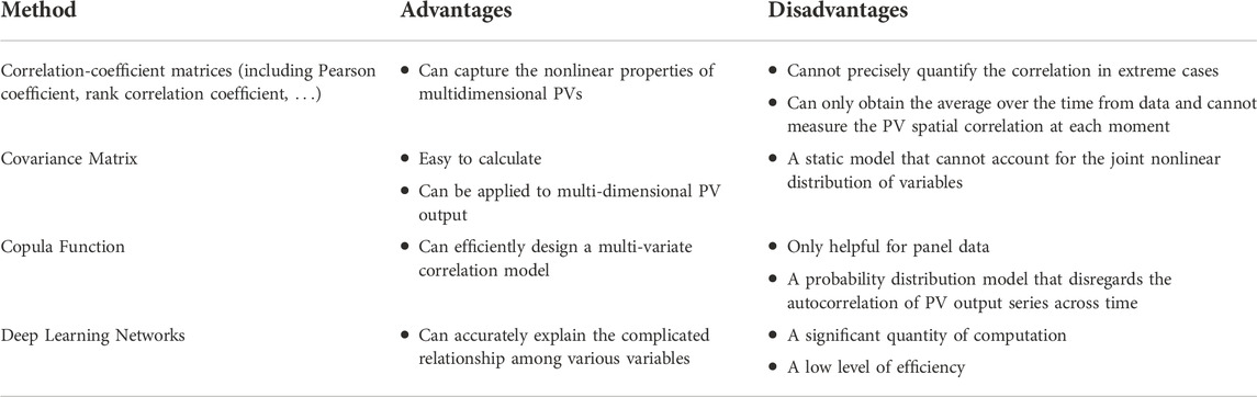
TABLE 1. Advantages and disadvantages of methods for constructing spatial correlation of PV output.

Second, the modeling of PV-output uncertainty in the optimal dispatching problem of an ADN is investigated. Stochastic optimization (SO) and robust optimization (RO) are the two primary forms of modeling optimization methodologies for PV-output uncertainty (Aharon and Laurent El, 2009). For instance, in (Liu et al., 2019), a day-ahead economic scheduling method based on chance-constrained programming was proposed considering the uncertainty of PV output. In (Vilaça Gomes et al., 2019), a new approach was formulated to model the uncertainty of the wind-sun-hydrothermal system by generating several representative scenarios. However, SO requires estimating the probability distribution of variables from historical data, which is prone to large errors in actual situations. In addition, considering the accurate representation of uncertainty, many scenarios may need to be considered, which will increase the computational complexity. Conversely, RO does not need to know the specific probability distribution, but given the values ranges of variables, that is, the uncertainty set (El-Meligy et al., 2022). In (Xu et al., 2020; Choi et al., 2022), the box uncertainty sets were used to restrict the upper and lower bounds of variables, which tend to be over-conservative. (Ji et al., 2019). and (Aghamohamadi et al., 2021) used the polyhedral uncertainty sets, which have a linear structure and can easily control the uncertain budget, to describe the uncertainties of PV outputs. However, it is difficult to depict the correlation between these parameters using box or polyhedral uncertainty sets. Significantly, the ellipsoidal uncertainty sets can effectively describe multi-type sets to facilitate data input and indicate the correlation between uncertain multi-variables (Chassein and Goerigk, 2016; Golestaneh et al., 2018). Considering the dynamic spatial correlation between multiple PV outputs, it is better to use an ellipsoidal uncertainty set to characterize the PV-output uncertainty in the robust optimization dispatching model of ADN.

Based on the above discussions, this study establishes a robust dispatching model for an ADN that fully considers the spatial correlation and uncertainty of PV output. In this model, the dynamic conditional correlation (DCC) generalized autoregressive conditional heteroskedasticity (DCC-GARCH) model is introduced to construct and predict multidimensional dynamic correlation coefficient models of PV outputs, representing temporal changes in spatial correlation. After modeling the dynamic spatial correlation, a time-varying ellipsoidal uncertainty set is introduced to bound the uncertainty of PV outputs. In addition, to build a highly reasonable and widely applicable ADN dispatching model, the coordination optimization of active and reactive power is considered, and a variety of methods are adopted to linearize the nonlinear constraints for an easy solution. Finally, the effectiveness and rationality of the proposed methodologies are demonstrated considering a rural ADN in China as an example. The major contributions of this study are as follows:

1) To characterize the time-varying characteristics of PV-output spatial correlation, the DCC-GARCH model is proposed in this study to establish a dynamic model of the correlation. The model also allows for intraday short-term forecasting of DCC, which can measure the spatial correlation.

2) To address the uncertainty problem of PV output in the optimization dispatching of an ADN, a time-varying ellipsoidal uncertain set based on the DCC-GARCH model is proposed to improve the robustness of photovoltaic output modeling. By introducing the uncertainty set, the MILP model for ADN optimal dispatching can be transformed into mixed integer robust optimization (MIRP).

The remainder of this paper is organized as follows. Section 2 describes the dynamic spatial correlation and proposes a time-varying spatial correlation model for the PV outputs. Section 3 explains the time-varying ellipsoidal uncertainty set of the PV outputs and constructs a robust dispatch model of ADN. In Section 4, the numerical results for a rural ADN in China are presented to verify the effectiveness of the proposed model. Finally, the conclusions are presented in Section 5.

2 Multidimensional dynamic spatial correlation model of PV output based on DCC-GARCH

2.1 Dynamic changes of PV output spatial correlation

Owing to the influence of micro-meteorology, PV power stations in the same area show different output variations. Relevant research has shown that there is a high correlation between the outputs of these PV stations, which is known as spatial correlation. The five PV stations in Zhangjiagang, Suzhou is taken as an example, which are shown in Figure 1. The PV output data in 2018 is used to draw Figure 2, which has been standardized by the installed capacity. And the sampling interval is 5 min.

FIGURE 1

FIGURE 1. Location of five PV stations.

FIGURE 2

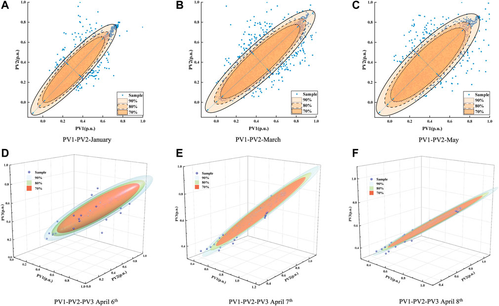
FIGURE 2. Power distribution and confidence interval of PV1-PV2 and PV1-PV2-PV3 at partial time. (A) PV1-PV2-January, (B) PV1-PV2-March, (C) PV1-PV2-May, (D) PV1-PV2-PV3 April 6th, (E) PV1-PV2-PV3 April 7th, and (F) PV1-PV2-PV3 April 8th.

Figure 2 displays the scatter plots of the power distribution of PVs at various time scales and dimensions, as well as the accompanying confidence intervals. As shown in Figure 2, the confidence ellipses of the same PVs at different times are considerably different, which implies that the spatial correlation of the same PVs varies over the time. In Figures 2A–C, the time scale is a month. The confidence ellipse for January is longer and thinner than those for March and May, resulting in a stronger spatial correlation. Figures 2D–F reflects the changes of three-dimensional (3D) confidence ellipses of PV1, PV2, and PV3 outputs across three consecutive days from April 6th to April 8th. On April 8th, the ellipsoid is the most elongated and has the shape of a prolate ellipsoid. Thus, the spatial correlation among the three PV stations is the strongest for the 3 days. In addition, on comparing Figures 2D–F with Figures 2A–C, it can be observed that the smaller the time scale is, the more noticeable is the fluctuation of spatial correlation of PV output.

Figure 2 illustrates that the spatial correlation of PV output has a significant time-varying feature, with the smaller time scale indicating a larger variation. However, most existing studies have built static models of spatial correlation and do not predict the spatial correlation itself. Based on this, a dynamic spatial-correlation model based on the DCC-GARCH model is proposed in this paper to realize the numerical characterization and prediction of spatial correlation with time-varying properties.

2.2 Dynamic spatial-correlation model and prediction based on DCC-GARCH

Suppose that the output time-series of k PV stations is ${\mathit{P}}_t^{PV}=[P_{1,t}^{PV},\dots P_{i,t}^{PV},\dots P_{K,t}^{PV}{]}^T$, where $P_{i,t}^{PV}$ denotes the output time series of the ith PV station. Defining the mean of $P_{i,t}^{PV}$ as ${\overline{P}}_{i,t}^{PV}$, the mean equation of each series is represented by the ARMA model, and the DCC-GARCH model of PV output spatial correlation is expressed as

${\overline{P}}_{i,t}^{PV}=c_i+{\displaystyle \sum }_{a=1}^{p_{arma}}{\phi }_{i,a}{\overline{P}}_{i,t-a}^{PV}+{\displaystyle \sum }_{b=1}^{q_{arma}}{\theta }_{i,b}{e}_{i,t-b}^{PV}(1)$

$h_{i,t}^{PV}={\omega }_i+{\displaystyle \sum }_{x=1}^p{\lambda }_{i,x}{\left(e_{i,t-x}^{PV}\right)}^2+{\displaystyle \sum }_{y=1}^q{\delta }_{i,y}\left(h_{i,t-y}^{PV}\right)(2)$

${\mathit{P}}_t^{PV}=\left[\begin{array}{c}{P}_{1,t}^{PV}\\ \cdots \\ P_{i,t}^{PV}\\ \cdots \\ P_{i,t}^{PV}\end{array}\right]={\overline{\mathit{P}}}_t^{PV}+{\mathit{e}}_t^{PV}(3)$

${\mathit{H}}_t^{PV}={\mathit{D}}_t^{PV}{\mathit{R}}_t^{PV}{\mathit{D}}_t^{PV}(4)$

${\mathit{D}}_t^{PV}=diag\left(\sqrt{h_{1,t}^{PV}},\cdot \cdot \cdot ,\sqrt{h_{i,t}^{PV}},\cdot \cdot \cdot ,\sqrt{h_{k,t}^{PV}}\right)(5)$

${\mathit{R}}_t^{PV}=\left[\begin{array}{cccc}{\rho }_{11}& {\rho }_{12}& \cdots & {\rho }_{1k}\\ {\rho }_{21}& {\rho }_{22}& \cdots & {\rho }_{2k}\\ \cdots & \cdots & \cdots & \cdots \\ {\rho }_{k1}& {\rho }_{k2}& \cdots & {\rho }_{kk}\end{array}\right]={\mathit{Q}}_t^{*-1}{\mathit{Q}}_t{\mathit{Q}}_t^{\ast -1}(6)$

${\mathit{Q}}_t=\left[\begin{array}{cccc}{q}_{11}& q_{12}& ...& q_{1k}\\ q_{21}& q_{22}& ...& q_{2k}\\ ...& ...& ...& ...\\ q_{2k}& ...& ...& q_{kk}\end{array}\right]=\left(1-{\displaystyle \sum }_{m=1}^M{\alpha }_m-{\displaystyle \sum }_{n=1}^N{\beta }_n\right)\overline{\mathit{Q}}+{\displaystyle \sum }_{m=1}^M{\alpha }_m{\mathit{\xi }}_{t-m}{\mathit{\xi }}_{t-m}^{\prime }+{\displaystyle \sum }_{n=1}^N{\beta }_n{\mathit{Q}}_{t-n}(7)$

$\overline{\mathit{Q}}=T^{-1}{\displaystyle \sum }_{t=1}^T{\mathit{\xi }}_t{\mathit{\xi }}_t^{\prime }(8)$

Equations 1, 2 establish the ARMA-GARCH model for the output of each PV station. Equation 1 is the mean equation using the ARMA model, and Equation 2 refers to the variance equation of the GARCH model, where the residual term {$e_{i,t}^{PV}$} is subject to N (0, $\sqrt{h_{i,t}^{PV}}$). $c_i$, $w_i$, ${\phi }_a$, ${\theta }_b$, ${\lambda }_x$ and ${\delta }_y$are constant coefficients. p_arma and q_arma are the orders of ARMA, and p and q are the lag orders of the GARCH. Eq. 3 is the variance equation, which can be calculated using the GARCH model. To ensure that the variance is positive, the parameters must satisfy ω_i > 0, λ_i,x >0, δ_j,y >0, and $\left({\displaystyle \sum }_{x=1}^p{\lambda }_{i,x}+{\displaystyle \sum }_{y=1}^q{\delta }_{i,y}\right)<1$.

Equations 3–8 build the DCC-GARCH model. In Eq. 3, $e_{i,t}^{PV}$ denotes the residual term, which is subject to N (0, $H_t^{PV}$). The covariance matrix $H_t^{PV}$ of $P_t^{PV}$can be decomposed into a DCC matrix $R_t^{PV}$ and two standard-deviation matrices $D_t^{PV}$, as shown in Equation 4. Eq. 6 defines $R_t^{PV}$ which is disintegrated into matrices ${\mathit{Q}}_t^{*}$ and Q_t.${\mathit{Q}}_t^{*}$ refers to a diagonal matrix whose elements are the square roots of the diagonal values of Q_t. In Eq. 8, ξ_t refers to a residual vector after standardization that satisfies ξ_t ${\left(D_t^{PV}\right)}^{-1}{\mathit{e}}_t^w$ $\overline{\mathit{Q}}$ is an unconditional variance matrix of ${\mathit{e}}_t^w$, satisfying Eq. 8.

The DCC (1,1)-GARCH (1,1) model is more frequently. In the simplified model, Eqs 2, 7 are simplified to Eqs 9, 10, respectively. The DCC can then be written as Eq. 11.

$h_{i,t}^{PV}={\omega }_i+{\lambda }_i{\left(e_{i,t-1}^{PV}\right)}^2+{\delta }_i\left(h_{i,t-1}^{PV}\right)(9)$

${\mathit{Q}}_t=\left(1-\alpha -\beta \right)\overline{\mathit{Q}}+\alpha {\mathit{\xi }}_{t-\mathit{1}}{\mathit{\xi }}_{t-1}^{\prime }+\beta {\mathit{Q}}_{t-\mathit{1}}(10)$

${\rho }_{ij,t}=\frac{q_{ij,t}}{\sqrt{q_{ii,t}{q}_{jj,t}}}=\frac{\left(1-\alpha -\beta \right){\overline{q}}_{ij}+\alpha {\xi }_{i,t-1}{\mathit{\xi }}_{j,t-1}+\beta q_{ij.t-1}}{\sqrt{\left(\left(1-\alpha -\beta \right){\overline{q}}_{ii}+\alpha {\xi }_{i,t-1}^2+\beta q_{ii.t-1}\right)\left(\left(1-\alpha -\beta \right){\overline{q}}_{jj}+\alpha {\xi }_{j,t-1}^2+\beta q_{jj.t-1}\right)}}(11)$

where ${\omega }_i$, ${\lambda }_i$, and δ_i are the parameters to be estimated in GARCH (1,1) and should be positive. α and β are positive parameters in DCC (1,1) and satisfy α + β < 1.

Consider the covariance matrix of r-step ahead prediction is

${\mathit{Q}}_{t+r}=\left(1-\alpha -\beta \right)\overline{\mathit{Q}}+\alpha {\mathit{\xi }}_{t+r-1}{\mathit{\xi }}_{t+r-1}^{\prime }+\beta {\mathit{Q}}_{t+r-1}(12)$

where $E_t\left[{\mathit{\xi }}_{t+r-1}{\mathit{\xi }}_{t+r-1}\right]$=$E_t\left[{\mathit{R}}_{t+r-1}^{PV}\right]{,{\mathit{R}}_{t+r}^{PV}=\mathit{Q}}_{t+r}^{*-\mathit{1}}{\mathit{Q}}_{t+r}{\mathit{Q}}_{t+r}^{*-\mathit{1}}$. Because of the nonlinearity, the prediction cannot be directly solved forward to provide a convenient method for prediction. Hence, an efficient method is proposed to generate the r-step ahead prediction of Q by approximating that $\overline{\mathit{Q}}$ ≈$\overline{\mathit{R}}$ and that $E_t\left[{\mathit{Q}}_{t+1}^{PV}\right]$=$E_t\left[{\mathit{R}}_{t+1}^{PV}\right]$ (Engle and Sheppard, 2001). Using this approximation, the DCC matrix RPV t can be predicted using the following relationship

$\begin{array}{l}{E}_t\left[{\mathit{R}}_{t+r}^{PV}\right]=E_t\left[{\mathit{Q}}_{t+r}\right]\\ ={\displaystyle \sum }_{i=0}^{r-2}\left(1-\alpha -\beta \right)\overline{\mathit{R}}{\left(\alpha +\beta \right)}^i+{\left(\alpha +\beta \right)}^{r-1}{\mathit{R}}_{t+1}\end{array}(13)$

So far, a dynamic spatial correlation model of PV output can be obtained. In addition to accurately describing the PV output, the model can also assess, compute, and predict the DCC of different PV outputs. In this study, the relative value ${\mathit{R}}_t^{PV}$ is used to characterize the DCC. The absolute value Q_t, which denotes the covariance matrix, is used to denote the time-varying ellipsoidal uncertainty set and solve the optimal dispatching model. ${\mathit{R}}_t^{PV}$ and Q_t are interconnected using Eq. 11.

3 Robust dispatching model for ADN considering the dynamic PV spatial correlation

In contrast to the transmission network, the resistance and reactance values of the ADN lines are close to each other, and the coupling between active and reactive power is strong (Sun et al., 2022). It is not sufficient to establish a unilateral active- or reactive-power dispatching model based on the traditional active- and reactive-power decoupling theory. The reactive-power resources about the high proportion of PV will affect the network loss and voltage quality (Antoniadou-Plytaria et al., 2017; Hu et al., 2022). Active power optimization can reduce generation costs, and reactive power regulation can reduce network losses, together achieving the goal of minimizing operating costs. Therefore, first, this section establishes the active- and reactive-power coordination dispatching model of the ADN. Thereafter, to facilitate the solution, the nonlinear constraints are linearized to form the MILP model. Finally, considering the uncertainty of PV output, a time-varying ellipsoid uncertainty set is proposed to construct a robust dispatching model of ADN.

3.1 Objective function

Because economy is a significant evaluation indicator for ADN, the lowest operating cost of ADN is chosen as the objective function in this paper. The operational expense consists of the cost of purchasing electricity from the grid, the dispatching cost of curtailable loads, and the lifespan-loss cost of the energy storage system (ESS), which is expressed as:

$\mathit{Min}F={\displaystyle \sum }_{t=1}^T\left(F^{buy}\left(t\right)+F^{CL}\left(t\right)\right)+F^{Ess}(14)$

$F^{buy}\left(t\right)={\displaystyle \sum }_i{m}^{buy}\left(t\right)P_{i,t}^{Load}\Delta t(15)$

$F^{CL}\left(t\right)={\displaystyle \sum }_i{m}_i^{CL}{P}_{i,t}^{CL}\Delta t(16)$

$F^{Ess}=\left({\pi }^{rep}-{\pi }^{res}\right)D{P}^{cy}(17)$

where F^buy(t) and F^CL(t) denote the cost of electricity purchase and dispatching cost of the curtailable load at time t, respectively, and F^Ess denotes the lifespan-loss cost of energy storage. In Eq. 15, m^buy(t) denotes the unit cost of electricity purchased from the upper grid. In Eq. 16, $m_i^{CL}$ denotes the demand-side response compensation cost. In Eq. 17, π^rep and π^res denote the replacement cost and residual value of the ESS, respectively, and DP^cy denotes the cycle degradation percentage of the ESS.

3.2 Constraints

The normal operation of the ADN must satisfy power flow constraints. To achieve reasonably coordinated dispatching within the system, it is also necessary to consider the operating constraints of each device. In this study, we consider the demand-side response constraints and the operating constraints of an ESS, on-load tap changer (OLTC), capacitor bank (CB), static var generator (SVG), and distributed generation (DG), as well as the impact of ESS lifespan losses on operational costs.

3.2.1 Power flow constraints

The injected and outflow powers at each node must be equal for the ADN. Therefore, the branch flow model can be expressed as

$\{\begin{array}{l}{P}_{ij,t}=\left(u_{i,t}^2-u_{i,t}{u}_{j,t}\cos {\theta }_{ij,t}\right)g_{ij}-u_{i,t}{u}_{j,t}{b}_{ij}\sin {\theta }_{ij,t}\\ Q_{ij,t}=-\left(u_{i,t}^2-u_{i,t}{u}_{j,t}\cos {\theta }_{ij,t}\right)b_{ij}-u_{i,t}{u}_{j,t}{g}_{ij}\sin {\theta }_{ij,t}\end{array}i,j\in B^{Node},t\in T(18)$

$\{\begin{array}{l}{P}_{i,t}={\displaystyle \sum }_{\left(i,j\right)}{P}_{ij,t}+\left({\displaystyle \sum }_{j=1}^N{G}_{ij}\right)v_{i,t}^2=P_{i,t}^{PV}+P_{i,t}^{Essdis}-P_{i,t}^{Esschar}\\ -\left(P_{i,t}^{Load}-P_{i,t}^{CL}\right)\\ Q_{i,t}={\displaystyle \sum }_{\left(i,j\right)}{Q}_{ij,t}+\left({\displaystyle \sum }_{j=1}^N-B_{ij}\right)v_{i,t}^2=Q_{i,t}^{PV}+Q_{i,t}^{Ess}+Q_{i,t}^{CB}+Q_{i,t}^{SVG}\\ -\left(Q_{i,t}^{Load}-P_{i,t}^{CL}\tan \varphi \right)\end{array}(19)$

$P_{ij,t}^2+Q_{ij,t}^2\le S_{ij,\max }^2(20)$

Eq. 18 gives the branch power flow equations, where θ_ij,t is the difference in the voltage phase angle between nodes i and j. g_ij and b_ij are the electric conductance and susceptance of branch ij, respectively. Eq. 19 shows the node power-balance equation, where G_ij and B_ij are the conductance and susceptance of the node to the ground, respectively. ϕ is the power-factor angle of the load being reduced. Eq. 20 constraints the capacity of branch ij.

3.2.2 OLTC operation constraints

OLTC can regulate the voltage by adjusting the position of the tap, which is an important component for maintaining voltage stability. A virtual node m can be added to the branches that contain OLTC to separate the transformer branch into an ideal transformer section and a lossy section.

The voltage of the ideal transformer on the secondary side can be expressed as

$u_{m,t}={\left({\delta }_{ij,t}\right)}^2{u}_{j,t},i,m,j\in B^{OLTC}(21)$

where δ_ij,t represents the turn ratio of the transformer branch at time t, which can be defined as a linear combination of the following constraints.

${\delta }_{ij,t}={\delta }_{ij}^{\mathit{min}}+T_{ij,t}\Delta {\delta }_{ij}(22)$

$\Delta {\delta }_{ij}=\left({\delta }_{ij}^{\mathit{max}}-{\delta }_{ij}^{\mathit{min}}\right)/K_{ij}(23)$

$0\le T_{ij,t}\le K_{ij}(24)$

where ${\delta }_{ij}^{\mathit{min}}$ and ${\delta }_{ij}^{\mathit{max}}$ are the minimum and maximum OLTC turn ratio, respectively. T_ij denotes the actual tap position, which is a non-negative integer variable. Δδ_ij is the change in turn ratio of each tap. K_ij denotes the maximum number of OLTC tap positions.

3.2.3 ESS operation constraints

$u_{i,t}^{char}+u_{i,t}^{dis}\le 1,\forall i\in B^{ESS},\forall t\in T(25)$

$\{\begin{array}{l}{u}_{i,t}^{char}\underset{¯}{P_i^{Esschar}}\le P_{i,t}^{Esschar}\le u_{i,t}^{char}\overline{P_i^{Esschar}}\\ u_{i,t}^{dis}\underset{¯}{P_i^{Essdis}}\le P_{i,t}^{Essdis}\le u_{i,t}^{dis}\overline{P_i^{Essdis}}\end{array}(26)$

$\{\begin{array}{l}SO{C}_{i,0}=SO{C}_{i,set}\\ SO{C}_{i,t}=SO{C}_{i,t-1}+(P_{i,t}^{Esschar}/{\eta }_i^{char}\Delta t\\ -P_{i,t}^{Essdis}/{\eta }_i^{dis}\Delta t)/E_i^{nomal}\\ \underset{¯}{SO{C}_i}\le SO{C}_{i,t}\le \overline{SO{C}_i}\\ SO{C}_{i,end}=SO{C}_{i,0}\end{array}\forall i\in B^{ESS},\forall t\in T(27)$

Constraints (25) and (26) limits the active power of the ESS at node i at time t. Constraint (27) limits the state of charge (SOC) at node i at time t. In constraint (27), $E_i^{nomal}$ is the rated capacity of the ith ESS. ${\eta }_i^{char}\mathrm{a}\mathrm{n}\mathrm{d}{\eta }_i^{dis}$ denote the charging and discharging efficiencies, respectively. To ensure that the ESS has the same operational performance in each scheduling cycle, it is assumed that the initial value of the SOC in this cycle is the same as the initial value of the SOC in the following cycle.

3.2.4 ESS cycle life loss constraints

The ESS loss cost accounts for a significant portion of the ADN operational cost. Because the ESS lifespan-loss might influence economic efficiency during operation, cyclic-life loss constraints for the ESS are constructed in this paper using the method proposed in the literature (Wang et al., 2016).

Assuming that the charging and discharging procedures have the same impact on the cycle lifespan degradation, a full charging and discharging cycle is divided into two distinct processes. The daily degradation is the sum of the degradations during each time interval, as shown in (28). For each period, the cycle lifespan degradation can be calculated by deducting the two regular degradations.

$D{P}^{cy}={\displaystyle \sum }_t{\mathrm{d}\mathrm{e}\mathrm{g}}_t^{cy}(28)$

${\mathrm{d}\mathrm{e}\mathrm{g}}_t^{cy}=0.5\left|{\mathrm{d}\mathrm{e}\mathrm{g}}_t-{\mathrm{d}\mathrm{e}\mathrm{g}}_{t-1}\right|(29)$

where deg_t denotes the cycle loss percentage corresponding to the SOC at time t, which can be obtained from the degradation-SOC curve, as shown in Wang et al. (2016).

Given that all the absolute values in Eq. 29 are less than 1, the nonlinear function can be converted into a linear inequality constraint by adding two binary variables d₁ and d₂. The functions are as follows:

$\{\begin{array}{l}0\le {\mathrm{d}\mathrm{e}\mathrm{g}}_t^{cy}-0.5\left({\mathrm{d}\mathrm{e}\mathrm{g}}_t-{\mathrm{d}\mathrm{e}\mathrm{g}}_{t-1}\right)\le 2d_2\\ 0\le {\mathrm{d}\mathrm{e}\mathrm{g}}_t^{cy}-0.5\left({\mathrm{d}\mathrm{e}\mathrm{g}}_{t-1}-{\mathrm{d}\mathrm{e}\mathrm{g}}_t\right)\le 2d_1\\ d_1+d_2=1\end{array}(30)$

3.2.5 CB and SVG constraints

Reactive-power-compensation components in an ADN typically fall into one of two types: the discrete component CB and the continuous component SVG. The constraints of the CB are as follows:

$\{\begin{array}{l}{y}_{i,t}^{CB}{Q}_i^{CB,step}=Q_{i,t}^{CB}\\ 0\le y_{i,t}^{CB}\le \overline{Y_i^{CB}}\\ y_{i,t}^{CB}\in \mathrm{i}\mathrm{n}\mathrm{t}\end{array}\forall t\in T,\forall i\in B^{CB}(31)$

$\{\begin{array}{l}{\displaystyle \sum }_{t\in T}{\delta }_{i,t}^{CB}\le N_i^{CB,\max }\\ -{\delta }_{i,t}^{CB}\overline{Y_i^{CB}}\le y_{i,t}^{CB}\le {\delta }_{i,t}^{CB}\overline{Y_i^{CB}}\end{array}\forall t\in T,\forall i\in B^{CB}(32)$

Constraint (32) constrains the number of operations, where where $N_i^{CB,\mathit{max}}$ is the upper limits of the operating quantity during each dispatching. ${\delta }_{i,t}^{CB}$ denotes the change in CB compensation capacity at adjacent moments.

SVG is a continuous reactive power compensation device that can effectively respond to the sudden changes in voltage or overvoltage caused by DG fluctuations in an ADN. The constraints of an SVG are as shown in Constraint (33):

$\begin{array}{cc}{Q}_i^{SVG,\min }\le Q_{i,t}^{SVG}\le Q_i^{SVG,\max }& \forall t\in T,\forall i\in B^{SVG}\end{array}(33)$

where $Q_i^{SVG,\mathit{min}}$ and $Q_i^{SVG,\mathit{max}}$ denote the lower and upper limits of SVG-compensated reactive power, respectively.

3.2.6 PV-output constraints

$\{\begin{array}{l}0\le P_{i,t}^{PV}\le \overline{P_{i,t}^{PV}}\\ -P_{i,t}^{PV}\tan \underset{¯}{\varphi }\le Q_{i,t}^{PV}\le P_{i,t}^{PV}\tan \overline{\varphi }\end{array}\forall t\in T,\forall i\in B^{PV}(34)$

$\begin{array}{cc}{\left(P_{i,t}^{PV}\right)}^2+{\left(Q_{i,t}^{PV}\right)}^2\le S_i^{PV}& \forall t\in T,\forall i\in B^{PV}\end{array}(35)$

The PV output constraints are presented in Constraints (34) and (35). Constraint (34) denotes the maximum PV active power at time t, whereas $\overline{\varphi }$ and $\underset{¯}{\varphi }$ are the maximum and minimum power factor angles, respectively. The maximum PV apparent power is limited by Constraint (35) to ensure system economy and safety.

3.2.7 Demand-response constraints

Demand response (DR) is crucial for ADN dispatch and optimization. It can reduce the uneven tide distribution caused by DG uncertainty. By tracking DG generation, DR can provide some regulation capability for the ADN. In this study, the main DR we considered is the curtailable load with the following constraints:

$\begin{array}{cc}{P}_{i,t}^{CL}\le q_{i,t}^{CL}{u}_{i,t}^{CL}& \forall i\in B^{CL},\forall t\in T\end{array}(36)$

$\begin{array}{cc}{\mathrm{y}}_{i,t}^{CL}-{\mathrm{z}}_{i,t}^{CL}=u_{i,t}^{CL}-u_{i,t-1}^{CL}& \forall i\in B^{CL},\forall t\in T\end{array}(37)$

$\begin{array}{cc}{\mathrm{y}}_{i,t}^{CL}{+\mathrm{z}}_{i,t}^{CL}\le 1& \forall i\in B^{CL},\forall t\in T\end{array}(38)$

$\begin{array}{cc}{\displaystyle \sum }_{t^{\prime }=t}^{t+TC{L}_{\min }^{CL}-1}{\mathrm{u}}_{i,t^{\prime }}^{CL}\ge TC{L}_{\min }^{CL}{y}_{i,t}^{CL}& \forall i\in B^{CL},\forall t\in T\end{array}(39)$

$\begin{array}{cc}{\displaystyle \sum }_{t^{\prime }=t}^{t+TC{L}_{\max }^{CL}-1}{\mathrm{z}}_{i,t^{\prime }}^{CL}\ge y_{i,t}^{CL}& \forall i\in B^{CL},\forall t\in T\end{array}(40)$

$\begin{array}{cc}{\displaystyle \sum }_{t\in T}{y}_{i,t}^{CL}\le Nu{m}^{CL}& \forall i\in B^{CL}\end{array}(41)$

where $q_{i,t}^{CL}$ is the maximum reduction per unit time for each curtailable load. $u_{i,t}^{CL}$ denotes the condition of load reduction, and $y_{i,t}^{CL}$ and ${\mathrm{z}}_{i,t}^{CL}$ denote that load reduction starts or stops, respectively, whereas all of them are binary variables. TCL^CL_min and TCL^CL_max are the minimum and maximum load-reduction times. Num^CL is the maximum quantity of loads that participates in the DR throughout the day.

3.3 Model linearization

3.3.1 Successive linear approximation of power flow

Despite the high computational accuracy of AC power flow, its non-convex nonlinear properties render it unsuitable for integration into complex distribution network optimization issues. Consequently, this study linearizes the power flow equation to improve the solution efficiency while maintaining appropriate computational accuracy. It then creates a linearized optimization model for an ADN.

Constraint (18) is nonlinear because of the product of a trigonometric function with the voltage. Suppose that an initial point (v_i,j,k, θ_i,j,k) is provided. The first-order Taylor series expansion of the sine and cosine functions is expressed as:

$\{\begin{array}{l}\sin {\theta }_{ij,t}\approx s_{ij,t,k}^1{\theta }_{ij,t,k}^1+s_{ij,t,k}^0\\ \cos {\theta }_{ij,t}\approx c_{ij,t,k}^1{\theta }_{ij,t,k}^1{+\mathrm{c}}_{ij,t,k}^0\end{array}(42)$

where,

$\{\begin{array}{l}{s}_{ij,t,k}^1=\cos {\theta }_{ij,t,k},s_{ij,t,k}^0=\sin {\theta }_{ij,t,k}-{\theta }_{ij,t,k}\cos {\theta }_{ij,t,k}\\ c_{ij,t,k}^1=-\sin {\theta }_{ij,t,k},{\mathrm{c}}_{ij,t,k}^0=\cos {\theta }_{ij,t,k}+{\theta }_{ij,t,k}\sin {\theta }_{ij,t,k}\end{array}(43)$

The power flow equation is formulated by incorporating (42) and (43) into Equation 18.

$\{\begin{array}{l}{P}_{ij,t}=v_{i,t}^2{g}_{ij}-v_{i,t}{v}_{j,t}\left(g_{ij}{\mathrm{c}}_{ij,t,k}^0+b_{ij}{\mathrm{s}}_{ij,t,k}^0\right)\\ -v_{i,t}{v}_{j,t}{\theta }_{ij,t}\left(g_{ij}{\mathrm{c}}_{ij,t,k}^1+b_{ij}{\mathrm{s}}_{ij,t,k}^1\right)\\ Q_{ij,t}=-v_{i,t}^2{b}_{ij}+v_{i,t}{v}_{j,t}\left(-g_{ij}{\mathrm{s}}_{ij,t,k}^0+b_{ij}{\mathrm{c}}_{ij,t,k}^0\right)\\ -v_{i,t}{v}_{j,t}{\theta }_{ij,t}\left(g_{ij}{\mathrm{s}}_{ij,t,k}^1-b_{ij}{\mathrm{c}}_{ij,t,k}^1\right)\end{array}(44)$

With $v_{i,t}^2$ as an integral variable, the nonlinear terms in the equation are v_i,tv_j,t and v_i,tv_j,tθ_ij,t. To decompose these two terms, we use the first-order Taylor expansion for θ_ij,t near the initial value, as shown in (45).

$v_{i,t}{v}_{j,t}{\theta }_{ij,t}\approx v_{i,t,k}{v}_{j,t,k}{\theta }_{ij,t}+\left(v_{i,t}{v}_{j,t}-v_{i,t,k}{v}_{j,t,k}\right){\theta }_{ij,t,k}(45)$

The v_i,tv_j,t can be uncoupled as (46). Subsequently, the first-order Taylor expansion can be used to further approximate the linearization of $v_{ij,t}^2$, as shown in (47).

$\begin{array}{l}{v}_{i,t}{v}_{j,t}=\frac{1}{2}\left[v_{i,t}^2+v_{j,t}^2-{\left(v_{i,t}-v_{j,t}\right)}^2\right]=\frac{v_{i,t}^2+v_{j,t}^2}{2}-\frac{v_{ij,t}^2}{2}\\ =\frac{U_{i,t}+U_{j,t}}{2}-\frac{v_{ij,t}^2}{2}\end{array}(46)$

$\begin{array}{l}{v}_{ij,t}^2\approx 2v_{ij,t,k}{v}_{ij,t}-v_{ij,t,k}^2\approx 2v_{ij,t,k}{v}_{ij,t}\frac{v_{i,t}+v_{j,t}}{v_{i,t,k}+v_{j,t,k}}-v_{ij,t,k}^2\\ =2\frac{v_{i,t,k}-v_{j,t,k}}{v_{i,t,k}+v_{j,t,k}}\left(v_{i,t}^2-v_{j,t}^2\right)-v_{ij,t,k}^2\\ =2\frac{v_{i,t,k}-v_{j,t,k}}{v_{i,t,k}+v_{j,t,k}}\left(U_{i,t}-U_{j,t}\right)-v_{ij,t,k}^2\\ =v_{ij,t,L}^s\end{array}(47)$

The linearized power flow constraints can be obtained by substituting (45)–(47) into (44), as follows:

$\{\begin{array}{l}{P}_{ij,t}^k=g_{ij}{U}_{i,t}-g_{ij}^{P,k}\frac{U_{i,t}+U_{j,t}}{2}-b_{ij}^{P,k}\left({\theta }_{ij,t}-{\theta }_{ij,t,k}\right)\\ +g_{ij}^{P,k}\frac{v_{ij,t,L}^s}{2}\\ Q_{ij,t}=-b_{ij}{U}_{i,t}+b_{ij}^{Q,k}\frac{U_{i,t}+U_{j,t}}{2}-g_{ij}^{Q,k}\left({\theta }_{ij,t}-{\theta }_{ij,t,k}\right)\\ -b_{ij}^{Q,k}\frac{v_{ij,t,L}^s}{2}\end{array}(48)$

where

$\{\begin{array}{l}{g}_{ij}^{P,k}=\left(g_{ij}{c}_{ij,k}^0+b_{ij}{s}_{ij,k}^0\right)+\left(g_{ij}{c}_{ij,k}^1+b_{ij}{s}_{ij,k}^1\right){\theta }_{ij,t,k}\\ b_{ij,k}^{P,k}=\left(g_{ij}{c}_{ij,k}^1+b_{ij}{s}_{ij,k}^1\right)v_{i,t,k}{v}_{j,t,k}\\ b_{ij}^{Q,k}=\left(-g_{ij}{s}_{ij,k}^0+b_{ij}{c}_{ij,k}^0\right)-\left(g_{ij}{s}_{ij,k}^1-b_{ij}{c}_{ij,k}^1\right){\theta }_{ij,t,k}\\ g_{ij,k}^{Q,k}=\left(g_{ij}{s}_{ij,k}^1-b_{ij}{c}_{ij,k}^1\right)v_{i,t,k}{v}_{j,t,k}\end{array}(49)$

In Yang et al. (2016) and Yang et al. (2017), it has been demonstrated by the examination of numerous instances that successive linear approximation of power flow has high accuracy. Its efficiency has a sizable advantage over heuristic methods owing to the rapid development of commercial linear-programming tools. Furthermore, compared with the second-order cone relaxation, the successive linear approximation, which is based on the Taylor series, has unrestricted objects and superior scalability.

3.3.2 Linearization of line capacity and DG capacity

Constraints (20), (35) are elliptical nonlinear constraints on capacity. Linearization can be realized using a linear approximation with multiple rectangular constraints.

The line capacity constraint is transformed into (50). The capacity constrained of DG inverter is transformed into (51).

$\{\begin{array}{c}-S_{ij,\max }\le P_{ij,t}\le S_{ij,\max }\\ -S_{ij,\max }\le Q_{ij,t}\le S_{ij,\max }\\ -\sqrt{2}{S}_{ij,\max }\le P_{ij,t}+Q_{ij,t}\le \sqrt{2}{S}_{ij,\max }\\ -\sqrt{2}{S}_{ij,\max }\le P_{ij,t}-Q_{ij,t}\le \sqrt{2}{S}_{ij,\max }\end{array}(50)$

$\begin{array}{cc}\{\begin{array}{c}-S_{i,t}^{DG}\le P_{i,t}^{DG}\le S_{i,t}^{DG}\\ -S_{i,t}^{DG}\le Q_{i,t}^{DG}\le S_{i,t}^{DG}\\ -\sqrt{2}{S}_{i,t}^{DG}\le P_{i,t}^{DG}+Q_{i,t}^{DG}\le \sqrt{2}{S}_{i,t}^{DG}\\ -\sqrt{2}{S}_{i,t}^{DG}\le P_{i,t}^{DG}-Q_{i,t}^{DG}\le \sqrt{2}{S}_{i,t}^{DG}\end{array}& \forall t\in T,\forall i\in B^{DG}\end{array}(51)$

3.3.3 Linearization of ESS cycle lifespan loss constraints

The constraints of the ESS cycle lifespan loss are non-convex and nonlinear and have integer variables. Through the second type of special-order sets (SOS2), the degradation-SOC curve can be linearized and is expressed as:

$So{C}_t={\displaystyle \sum }_m{\Delta }_{t,m}So{C}_{t,m}(52)$

${\mathrm{d}\mathrm{e}\mathrm{g}}_t={\displaystyle \sum }_m{\Delta }_{t,m}{\mathrm{d}\mathrm{e}\mathrm{g}}_{t,m}(53)$

${\displaystyle \sum }_m{\Delta }_{t,m}=1(54)$

${\displaystyle \sum }_m{\delta }_{t,m}=1(55)$

${\Delta }_{t,m}\le {\delta }_{t,m}+{\delta }_{t,m-1}(56)$

where m is the number of SOC-curve segments of the ESS. Δ_t,m and δ_t,m are the SOS2 variables at time t.

3.4.4 Linearization of OLTC operating constraints

There are integer variables in the OLTC constraints. To avoid the dimensional disaster caused by the non-deterministic polynomial (NP) problem, the OLTC constraints are linearized using following procedure:

Suppose λ_ij,t,n is a binary variable,

$T_{ij,t}={\displaystyle \sum }_{n=0}^{N_{ij}}{2}^n{\lambda }_{ij,t,n}(57)$

where

$\underset{N_{ij}}{\min }{\displaystyle \sum }_{n=0}^{N_{ij}}{2}^n,s.t.{\displaystyle \sum }_{n=0}^{N_{ij}}{2}^n\ge K_{ij}(58)$

While defining m_ij,t = δ_ij,tU_j,t, h_ij,t = λ_ij,t,nU_j,t, and g_ij,t,n = λ_ij,t,nm_ij,t, Eqs 59, 60 can be respectively obtained by multiplying both sides of Equation 22 by U_j,t and m_ij,t.

$m_{ij,t}={\delta }_{ij}^{\min }{U}_{j,t}+\mathrm{\Delta }{\delta }_{ij}{\displaystyle \sum }_{n=0}^{N_{ij}}{2}^n{h}_{ij,t}(59)$

${\delta }_{ij,t}{m}_{ij,t}={\delta }_{ij}^{\min }{m}_{ij,t}+\mathrm{\Delta }{\delta }_{ij}{\displaystyle \sum }_{n=0}^{N_{ij}}{2}^n{g}_{ij,t,n}(60)$

Using the Big-M method, two equivalences can be achieved by introducing a large number M:

$h_{ij,t}={\lambda }_{ij,t,n}{U}_{j,t}\Rightarrow \{\begin{array}{c}0\le U_{j,t}-h_{ij,t}\le \left(1-{\lambda }_{ij,t,n}\right)M\\ 0\le h_{ij,t}\le {\lambda }_{ij,t,n}M\end{array}(61)$

$g_{ij,t,n}={\lambda }_{ij,t,n}{m}_{ij,t}\Rightarrow \{\begin{array}{c}0\le m_{ij,t}-g_{ij,t,n}\le \left(1-{\lambda }_{ij,t,n}\right)M\\ 0\le g_{ij,t,n}\le {\lambda }_{ij,t,n}M\end{array}(62)$

Thus far, OLTC operation constraints have been linearized, converting the model to a mixed integer model. Additionally, daily modifications of the OLTC must be restricted, as shown in (63).

$\{\begin{array}{l}{\delta }_{ij,t,up}+{\delta }_{ij,t,do}\le 1\\ {\displaystyle \sum }_{n=0}^{N_{ij}}{2}^n{\lambda }_{ij,t,n}-{\displaystyle \sum }_{n=0}^{N_{ij}}{2}^n{\lambda }_{ij,t-1,n}\ge {\delta }_{ij,t,up}-{\delta }_{ij,t,do}{K}_{ij}\\ {\displaystyle \sum }_{n=0}^{N_{ij}}{2}^n{\lambda }_{ij,t,n}-{\displaystyle \sum }_{n=0}^{N_{ij}}{2}^n{\lambda }_{ij,t-1,n}\le {\delta }_{ij,t,up}-{\delta }_{ij,t,do}\\ {\displaystyle \sum }_{t\in T}{\delta }_{ij,t,up}+{\delta }_{ij,t,do}\le N_j^{\max }\end{array}(63)$

where δ_ij,t,up and δ_ij,t,do are binary variables that define the increasing and decreasing of OLTC ratio at time t. $N_j^{\mathit{max}}$ is the maximum time of changes during operation.

3.4 Time-varying ellipsoidal uncertainty set of PVs

It is vital to describe the uncertainty set for many optimizations dispatching problems based on robust optimization. Among the different ways to contribute to uncertainty sets, the box uncertainty set is over conservative, and the polyhedral uncertainty set cannot express the correlation between uncertain parameters. Therefore, a more flexible ellipsoidal uncertainty set is adopted to describe the uncertainty of PV output. The specific ellipsoidal uncertainty set is as follows

${\mathrm{\Psi }}^{\alpha }:{\left({\mathit{X}}_t^{PV}-{\overline{\mathit{X}}}_t^{PV}\right)}^T{\Sigma }^{-1}\left({\mathit{X}}_t^{PV}-{\overline{\mathit{X}}}_t^{PV}\right)\le {\mathrm{\Gamma }}^{\alpha }(64)$

where ${\mathit{X}}_t^{PV}$ denotes a multivariate PV-output variable of dimension k at time t that can be forecasted by historical PV output data, and ${\overline{\mathit{X}}}_t^{PV}$ is the mean value of ${\mathit{X}}_t^{PV}$; $\Sigma$ is the predicted covariance matrix, which is obtained from the historical data; ${\Gamma }^{\alpha }$, which is usually called the uncertainty budget, denotes the coverage rate of observations.

In this study, the ARMA model is used to obtain the PV output predicted value ${\overline{\mathit{X}}}_t^{PV}$ of dimension k at every time t. The covariance matrix Q_t predicted using DCC-GARCH is regarded as $\Sigma$, which changes over time and represents the spatial correlation of different PVs. The uncertainty budget, which controls the robustness of the optimization model, is chosen by different confidence levels of the PV output data.

${\mathrm{\Psi }}^{\alpha }:{\left({\mathit{X}}_t^{PV}-{\overline{\mathit{X}}}_t^{PV}\right)}^T{\mathit{Q}}_t^{-1}\left({\mathit{X}}_t^{PV}-{\overline{\mathit{X}}}_t^{PV}\right)\le {\mathrm{\Gamma }}^{\alpha }(65)$

3.5 Solution method

Through the modeling process of Sections 3.1–Sections 3.2, we obtained the active and reactive power coordination dispatching model of the ADN. After the linearization process of the constraints mentioned in Section 3.3, the model proposed in this study is transformed into a mixed integer linear programmed (MILP) optimization model.

Considering the uncertainty of PV output, the time-varying ellipsoidal uncertainty set was developed in Section 3.4. Introducing this set, a robust constraint, into the MILP model, we can obtain a mixed integer robust programmed (MIRP) optimization model that can be computed using solvers. The detailed flowchart of modeling process in this study is presented as Figure 3.

FIGURE 3

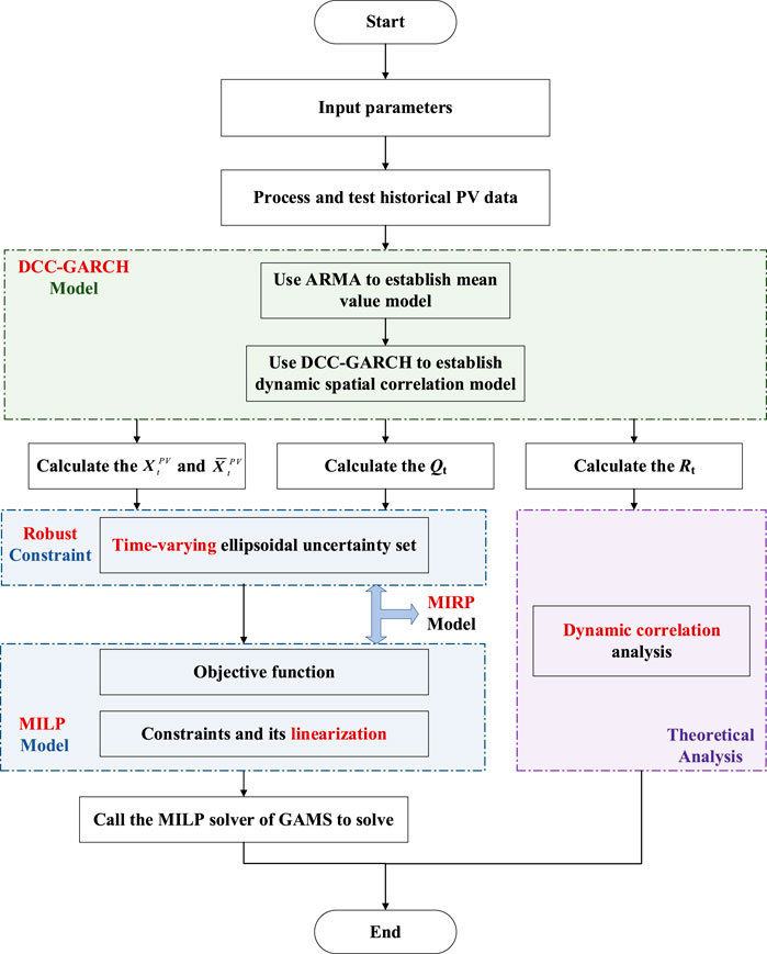
FIGURE 3. Flowchart of the robust dispatching model of ADN considering PV time-varying spatial correlation

4 Case studies

4.1 Dynamic spatial correlation model and prediction based on DCC-GARCH

First, the dynamic spatial correlation model of PV output is analyzed, and the data are from the output of PV system in Figure 1 in Suzhou, China. The data of March 1–24 in 2018, during which the weather was sunny, were selected for modeling and prediction. The interval was set to 20 min from 8:00 to 16:00, which can display the changes in the spatial correlation between PVs. After the Augmented Dickey-Fuller (ADF) test, normality, and Lagrange multiplier (LM) test, the results indicate that the historical PV data can be modeled using ARMA and DCC-GARCH, with the ARMA model of PV output being shown in Supplementary Table S1. The parameters of the five-dimensional DCC-GARCH model being shown in Table 2.

TABLE 2

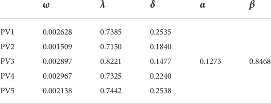
TABLE 2. Parameters of five-dimensional DCC-GARCH model.

The standardized residual series were re-evaluated after the model was constructed. The results indicated no correlation between variables, proving that the model had successfully eliminated the autocorrelation and heteroscedasticity of the data itself. As shown in Table 2, α and β are positive. The sum of α and β (0.974) is less than 1, which indicates that the model is stable, and there is a valid dynamic correlation between the five PVs. Parameter α indicates the influence of the current residual on the time series volatility at the next moment, and a higher α indicates that the time series is more sensitive to the recent residual. Parameter α +β indicates the disappearance speed of current fluctuations in the future, namely, the duration of the spatial correlation of PV output. The higher the value α +β is, the longer is the correlation duration. From Table 2, the result of fitting β is larger than α, indicating that the current dynamic heteroscedasticity of each series arises mainly from the residual of the previous period. The sum of α+β is close to 1, which implies that the spatial correlation has strong continuity.

The DCC matrix R_t of the PV output was calculated using the DCC-GARCH model, with the DCC curve between two pairs under 20 min time resolution being drawn as shown in Figure 4 below.

FIGURE 4

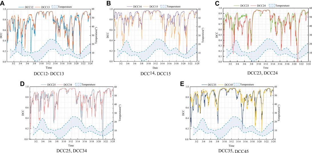
FIGURE 4. DCC diagrams of PV output. (A) DCC12, DCC13, (B) DCC14, DCC15, (C) DCC23, DCC24, (D) DCC25, DCC34, and (E) DCC35, DCC45.

According to the comparison between Figure 1 and Table 3, it can be observed that distance is one of the factors that affect DCC. The closer the PVs are, the higher is the DCC value. Otherwise, owing to the dynamic change of DCC, the spatial correlation between the two PVs shows different magnitude relationships at different times. This phenomenon is mainly related to temperature and weather.

TABLE 3

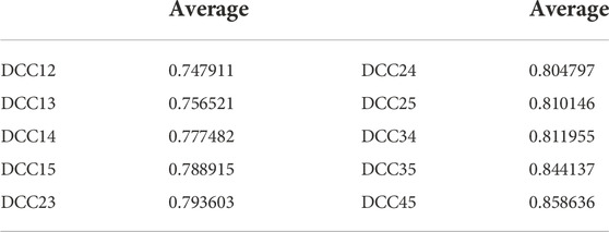
TABLE 3. The average DCC of different PVs.

Comparing Figure 4 with the weather conditions shown in Supplementary Table S2, the maximum and minimum temperatures varied significantly from March 9 to 13. However, the temperature difference remained largely the same owing to five consecutive days of partly cloudy weather. Therefore, the DCC was mainly above 0.9, indicating a high spatial correlation among the PVs during this period. Additionally, the DCC varied dramatically owing to the more pronounced temperature difference fluctuations on March 1–7 and March 5–21. On these days, the weather in the location was cloudy and rainy.

Therefore, the following conclusions can be drawn: When the temperature difference fluctuates more steadily, the DCC changes smoothly, and the DCC is more prominent when the weather is fine. When the temperature difference fluctuates sharply, usually accompanied by inclement weather, the change in solar radiation causes a considerable change in the PV output, which in turn causes a variation in the DCC.

Data from March 1 to 24 were used as the test set, and the forecast step was set to 24. The DCC-GARCH model was used for the rolling forecast to obtain the DCC from 8:00 to 16:00 on March 25 (with an interval of 20 min). The predicted values of the DCC are compared with the actual values in Figure 5, and the mean square error (MSE) is shown in Supplementary Table S3. It can be observed that the errors are within the acceptable range, and the prediction results are accurate. However, in most instances, the prediction values are more prominent than the actual values because of the rapid variation in cloud cover.

FIGURE 5

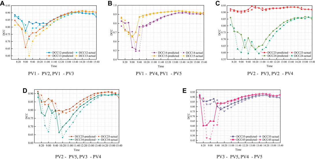
FIGURE 5. Comparison of DCC predicted value and actual value. (A) PV1-PV2, PV1-PV3, (B) PV1-PV4, PV1-PV5, (C) PV2-PV3, PV2-PV4, (D) PV2-PV5, PV3-PV4, and (E) PV3-PV5, PV4-PV5.

4.2 Case description

Robust ADN dispatching is verified in the next section. The grid structure is abstracted from a rural distribution network in Anhui, China, as shown in Figure 6. There are five PV stations (different from Figure 1), one ESS, one SVG, and three CBs. The case uses 24 h as the dispatch period and 60 min as the dispatch interval. The capacities of the PV stations were set to 3MW, 2.4MW, 2MW, 2.4MW, and 4 MW. The parameters of the ESS are as follows: The ESS capacity is 1MW; the initial charge state SOC_i,0 is 0.5; ${\eta }_i^{char}and{\eta }_i^{dis}$, the efficiency of charging and discharging, are set to 88% and 90%, respectively; and the depth of discharge is 90%. For the OLTC (at node one), the maximum number of OLTC tap positions K_ij was set to 16. $d_{ij}^{\mathit{min}}\mathrm{a}\mathrm{n}\mathrm{d}{d}_{ij}^{\mathit{max}}$ were set to 0.857 and 1.048, respectively. For the DR, the compensation cost value was set to 100 yuan/MWh. Additionally, the electricity price purchased from the power grid adopts a peak-to-valley sales tariff. The load in the system includes residential and agricultural loads.

FIGURE 6

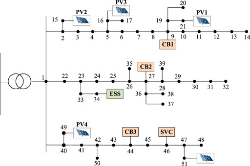
FIGURE 6. A typical rural distribution system.

To verify the significance of considering the time-varying characteristic of the PV-output spatial correlation, the numerical tests were mainly conducted in the following two cases:

Case A. Robust dispatching model for the ADN without considering the time-varying characteristics of PV-output spatial correlation.

Case B. Robust dispatching model for the ADN with time-varying characteristic consideration of PV-output spatial correlation.

4.3 Dispatching results for case A

When the time-varying characteristic of PV-output spatial correlation is not considered, the correlation coefficients among the five PVs can easily be derived from the Pearson coefficient. In this case, the ellipsoidal uncertainty set is static, as shown in Eq. 64. The objective function and related parameters can be determined as follow:

Figure 7A depicts the PV output curves, and Figure 7B illustrates the active power changes of PCC and the SOC curves of ESS for Case A. It can be observed that when the time-varying spatial correlation is ignored, the PV-output curves are jagged. Some PV-power valleys occur around midday, which leads to the apparent fluctuations of the PCC active power in Figure 7B. To secure the balance of power supply for the entire system, the SOC state of ESS begins charging immediately at 12:00 when the PV output is low and reaches full power at 13:00. The full power condition lasts for nearly 7 h to guarantee that the load is supplied throughout the night so that the objective function is minimized to the greatest extent.

FIGURE 7

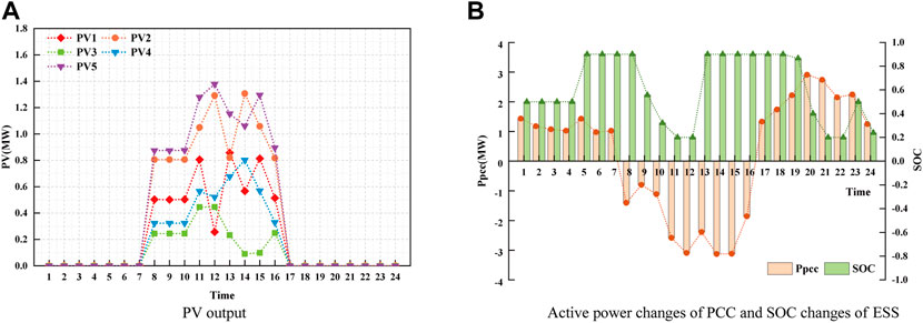
FIGURE 7. Partial-component-change curves for Case A. (A) PV output, (B) Active power changes of PCC and SOC changes of ESS.

The maximum number of OLTC changes within the dispatching period was set to no more than two. Three CBs were connected to nodes 9, 27, and 44. The maximum number of access CB groups was set to five, and the maximum number of changes was two. As shown in Supplementary Figure S1, the variations in OLTC and CB both satisfied the limits. The maximum number of access CB groups during the dispatching period was five. This means that a high proportion of PV in the ADN will cause reactive power shortages and other problems, requiring timely action of reactive-power compensation equipment to ensure stable system operation. In the proposed coordinated dispatching model of ADN, OLTC and CB operate together with the ESS to achieve active management of the ADN and always ensure the voltage quality of the entire system supply.

4.4 Dispatching results for case B

Considering the dynamic trait of PV-output spatial correlation, the covariance matrix Q_t, interconnected with the DCC by Eq. 11, can be used in the uncertainty set, where the time-varying ellipsoidal uncertainty set is obtained, as shown in Eq. 65. In addition, because the dispatching interval is 1 h, the PV output time was set as 8:00–16:00, according to the actual situation. The covariances between PVs are shown in Supplementary Figure S2, which indicates the spatial correlation variation. The covariance curves for different PVs share a similar trend: a strong correlation at noon and a weak correlation in the morning and evening, which is caused by the illumination intensity and temperature.

Subsequently, a model for the robust dispatching of ADN that considers time-varying spatial correlation was developed. Considering the influence of different uncertainty budgets on the ellipsoidal uncertainty set, the objective function and related parameters were obtained under different uncertainty budgets, as listed in Table 5, where the PV consumption rate is the ratio of the actual output to the ideal output.

First, the effect of time-varying spatial correlation is considered. Comparing Table 5 with Table 4, without time-varying spatial correlation, it can be observed that the total cost of operation increases owing to the reduction in PV output, which increases the cost of power purchase from the upper grid. On the other hand, the decrease in PV output affects the charging and discharging status of the ESS, thus reducing the ESS benefits.

TABLE 4

TABLE 4. Dispatching results of MILP.

Figure 8 illustrates the PV output, and Figure 9 reveals the active power changes at the point of common coupling (PCC) at node 1 and the SOC tendencies of the ESS. Compared with Figure 7, under any uncertainty budget, the curves of the PV output and PCC output are smoother, and the value of the PV output at each node is higher when the time-varying spatial correlation is considered. In Figure 8, the PCC output is in the trend of the morning and evening peaks and noon trough. Because most of the loads are residential loads, the peak period of electricity consumption is from 20:00 to 22:00. During this period, the PCC output reaches its peak, and the ESS is in a discharged state to ensure the load supply. The SOC curves indicate that the ESS is releasing energy during the morning peak of electricity consumption after 7 a.m. and charges during the peak of the PV generation. In conclusion, considering the time-varying spatial correlation of PVs is helpful for comprehensively evaluating the output characteristics of PV and optimizing the dispatching results.

FIGURE 8

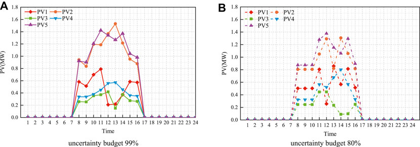
FIGURE 8. PV output under different uncertainty budget for Case B. (A) uncertainty budget 99%, (B) uncertainty budget 80%.

FIGURE 9

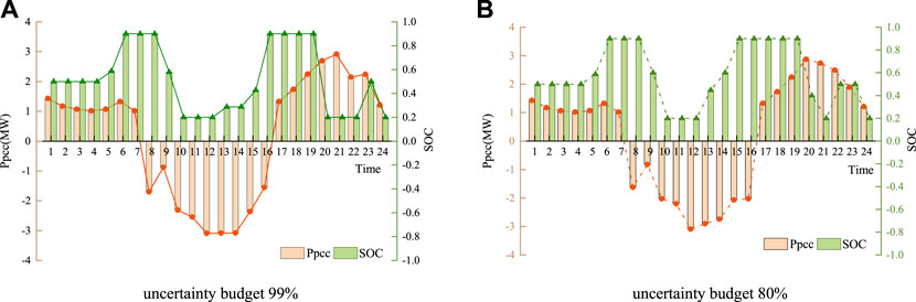
FIGURE 9. Active power changes of PCC and SOC changes of ESS for Case B. (A) uncertainty budget 99%, (B) uncertainty budget 80%.

Secondly, we consider the influence of the uncertainty budget. As can be observed from Table 5, as the uncertainty budget increases, the overall operating cost decreases, and the PV consumption rate increases progressively. This is caused by the selection of the uncertainty budget influencing the robustness of the system operation: the greater the uncertainty budget is, the more points are included in the ellipsoidal uncertainty set, and similarly, the more conservative are the results (Wu et al., 2022). Because the total cost of operation only includes the cost of power purchase and energy storage operation, not the cost of PV operation, to minimize the objective function, a high PV output caused by the high uncertainty budget will become the main power supply of the grid, which will reduce the cost of power purchase from the upper grid and the total cost of operation. Under different circumstances, the network loss varies based on the dispatching status of the PV output and the upper-grid supply.

TABLE 5

TABLE 5. Results of robust dispatching.

Under uncertainty budgets of 99% and 80%, Figures 8, 9 shows quite different curves. When the uncertain budget is 99%, the output value of the PV at each moment is slightly larger than that under the 80% budget, and the output curve of the PCC is smoother. Because the total operating cost considers the lifespan loss cost of the ESS, to minimize the objective function as much as possible, the charging and discharging times of the ESS are reduced under an uncertainty budget of 99% with higher conservatism.

Because the case is a rural distribution network, a low load demand is accompanied by high PV penetration. In the high PV output period, combining the peak–valley spread revenue of the ESS, surplus power will be sold to the upper grid at the purchase price. This approach can improve the PV consumption rate and result in PCC power for negative values from 8:00 to 16:00. In the entire dispatching process with an uncertainty budget of 99%, the ESS benefit is 649.108 yuan, which appropriately reduces the total operation cost.

In the daytime, the voltage of each node connected to the PV system increases significantly, as shown in Supplementary Figure S3. Owing to the PV power cut-in at 8:00 and cut-out at 16:00, all five node voltages exhibited considerable fluctuations. Additionally, more PVs with larger capacities were connected to Line I, resulting in a higher overall node voltage than that of Line III.

5 Conclusion

In this study, a robust dispatching model for an ADN was proposed, which considers PV-output spatial correlation and uncertainty. A dynamic spatial correlation model was proposed to characterize the time-varying characteristics of PV output spatial correlation. Based on this, a time-varying ellipsoidal uncertain set was constructed and applied to the ADN dispatching model, which improved the robustness of PV-output model. Case studies on a rural distribution network in China demonstrated the validity and rationality of the proposed methods. The results indicated that:

(1) The DCC derived using the DCC-GARCH model correctly characterized the spatial correlation of PV output and reflected the time-varying properties of the spatial correlation.

(2) The value of DCC is related to the weather conditions and temperature difference in the area where the PV is located: When the temperature difference swings more consistently, the DCC changes more smoothly; When the weather is favorable, the DCC is greater. When the temperature difference varies dramatically, which is generally accompanied by severe weather, the DCC also changes.

(3) The time-varying ellipsoidal uncertainty set constructed using the DCC can be well applied to the optimal dispatching model of ADN. Considering the time-varying characteristics of the spatial correlation, it is advantageous to build a complete PV output model and optimize the dispatching results.

Data availability statement

The original contributions presented in the study are included in the article/Supplementary Material, further inquiries can be directed to the corresponding author.

Author contributions

XM: Methodology, analysis, and writing. HW: Conceptualization, software, review, and editing. YY: supervision, review, and editing.

Funding

This work is supported by the Major Basic Research Project of the Natural Science Foundation of the Jiangsu Higher Education Institutions of China (22KJD470003).

Conflict of interest

The authors declare that the research was conducted in the absence of any commercial or financial relationships that could be construed as a potential conflict of interest.

Publisher’s note

All claims expressed in this article are solely those of the authors and do not necessarily represent those of their affiliated organizations, or those of the publisher, the editors and the reviewers. Any product that may be evaluated in this article, or claim that may be made by its manufacturer, is not guaranteed or endorsed by the publisher.

Supplementary material

The Supplementary Material for this article can be found online at: https://www.frontiersin.org/articles/10.3389/fenrg.2022.1012581/full#supplementary-material

References

Aghamohamadi, M., Mahmoudi, A., and Haque, M. H. (2021). Two-stage robust sizing and operation co-optimization for residential PV–battery systems considering the uncertainty of PV generation and load. IEEE Trans. Ind. Inf. 17, 1005–1017. doi:10.1109/TII.2020.2990682

CrossRef Full Text | Google Scholar

Aharon, B.-T., and Laurent El, G. (2009). Robust optimization. Princeton: Princeton University Press.

Google Scholar

Antoniadou-Plytaria, K. E., Kouveliotis-Lysikatos, I. N., Georgilakis, P. S., and Hatziargyriou, N. D. (2017). Distributed and decentralized voltage control of smart distribution networks: Models, methods, and future research. IEEE Trans. Smart Grid 8, 2999–3008. doi:10.1109/TSG.2017.2679238

CrossRef Full Text | Google Scholar

Calcabrini, A., Ziar, H., Isabella, O., and Zeman, M. (2019). A simplified skyline-based method for estimating the annual solar energy potential in urban environments. Nat. Energy 4, 206–215. doi:10.1038/s41560-018-0318-6

CrossRef Full Text | Google Scholar

Chassein, A., and Goerigk, M. (2016). Min-max regret problems with ellipsoidal uncertainty sets. arXiv: Optimization and Control. doi:10.48550/arXiv.1606.01180

CrossRef Full Text | Google Scholar

Choi, J., Lee, J.-I., Lee, I.-W., and Cha, S.-W. (2022). Robust PV-BESS scheduling for a grid with incentive for forecast accuracy. IEEE Trans. Sustain. Energy 13, 567–578. doi:10.1109/TSTE.2021.3120451

CrossRef Full Text | Google Scholar

Ding, F., and Mather, B. (2017). On distributed PV hosting capacity estimation, sensitivity study, and improvement. IEEE Trans. Sustain. Energy 8, 1010–1020. doi:10.1109/TSTE.2016.2640239

CrossRef Full Text | Google Scholar

El-Meligy, M. A., El-Sherbeeny, A. M., and Anvari-Moghaddam, A. (2022). Transmission expansion planning considering resistance variations of overhead lines using minimum-volume covering ellipsoid. IEEE Trans. Power Syst. 37, 1916–1926. doi:10.1109/TPWRS.2021.3110738

CrossRef Full Text | Google Scholar

Engle, R., and Sheppard, K. (2001). Theoretical and empirical properties of dynamic conditional correlation multivariate GARCH. Cambridge, MA: National Bureau of Economic Research.

Google Scholar

Golestaneh, F., Pinson, P., Azizipanah-Abarghooee, R., and Gooi, H. B. (2018). Ellipsoidal prediction regions for multivariate uncertainty characterization. IEEE Trans. Power Syst. 33, 4519–4530. doi:10.1109/TPWRS.2018.2791975

CrossRef Full Text | Google Scholar

Haque, M. M., and Wolfs, P. (2016). A review of high PV penetrations in LV distribution networks: present status, impacts and mitigation measures. Renew. Sustain. Energy Rev. 62, 1195–1208. doi:10.1016/j.rser.2016.04.025

CrossRef Full Text | Google Scholar

Hu, R., Wang, W., Wu, X., Chen, Z., Jing, L., Ma, W., et al. (2022). Coordinated active and reactive power control for distribution networks with high penetrations of photovoltaic systems. Sol. Energy 231, 809–827. doi:10.1016/j.solener.2021.12.025

CrossRef Full Text | Google Scholar

Ji, H., Wang, C., Li, P., Ding, F., and Wu, J. (2019). Robust operation of soft open points in active distribution networks with high penetration of photovoltaic integration. IEEE Trans. Sustain. Energy 10, 280–289. doi:10.1109/TSTE.2018.2833545

CrossRef Full Text | Google Scholar

Liu, H., Zhang, Y., Ge, S., Gu, C., and Li, F. (2019). Day-ahead scheduling for an electric vehicle PV-based battery swapping station considering the dual uncertainties. IEEE Access 7, 115625–115636. doi:10.1109/ACCESS.2019.2935774

CrossRef Full Text | Google Scholar

Luo, Y., Yang, D., Yin, Z., Zhou, B., and Sun, Q. (2020). Optimal configuration of hybrid-energy microgrid considering the correlation and randomness of the wind power and photovoltaic power. IET Renew. Power Gener. 14, 616–627. doi:10.1049/iet-rpg.2019.0752

CrossRef Full Text | Google Scholar

Pan, C., Wang, C., Zhao, Z., Wang, J., and Bie, Z. (2019). A copula function based monte Carlo simulation method of multivariate wind speed and PV power spatio-temporal series. Energy Procedia 159, 213–218. doi:10.1016/j.egypro.2018.12.053

CrossRef Full Text | Google Scholar

Sun, X., Qiu, J., Tao, Y., Ma, Y., and Zhao, J. (2022). Coordinated real-time voltage control in active distribution networks: An incentive-based fairness approach. IEEE Trans. Smart Grid 13, 2650–2663. doi:10.1109/TSG.2022.3162909

CrossRef Full Text | Google Scholar

Vilaça Gomes, P., Saraiva, J. T., Carvalho, L., Dias, B., and Oliveira, L. W. (2019). Impact of decision-making models in transmission expansion planning considering large shares of renewable energy sources. Electr. Power Syst. Res. 174, 105852. doi:10.1016/j.epsr.2019.04.030

CrossRef Full Text | Google Scholar

Wang, Y., Zhou, Z., Botterud, A., Zhang, K., and Ding, Q. (2016). Stochastic coordinated operation of wind and battery energy storage system considering battery degradation. J. Mod. Power Syst. Clean. Energy 4, 581–592. doi:10.1007/s40565-016-0238-z

CrossRef Full Text | Google Scholar

Wu, H., Yuan, Y., Zhang, X., Miao, A., and Zhu, J. (2022). Robust comprehensive PV hosting capacity assessment model for active distribution networks with spatiotemporal correlation. Appl. Energy 323, 119558. doi:10.1016/j.apenergy.2022.119558

CrossRef Full Text | Google Scholar

Wu, H., Yuan, Y., Zhu, J., Qian, K., and Xu, Y. (2021). Potential assessment of spatial correlation to improve maximum distributed PV hosting capacity of distribution networks. J. Mod. Power Syst. Clean Energy 9, 800–810. doi:10.35833/MPCE.2020.000886

CrossRef Full Text | Google Scholar

Xu, S., Sun, H., Zhao, B., Yi, J., Hayat, T., Alsaedi, A., et al. (2020). The integrated design of a novel secondary control and robust optimal energy management for photovoltaic-storage system considering generation uncertainty. Electronics 9, 69. doi:10.3390/electronics9010069

CrossRef Full Text | Google Scholar

Yang, Z., Bose, A., Zhong, H., Zhang, N., Xia, Q., and Kang, C. (2017). Optimal reactive power dispatch with accurately modeled discrete control devices: A successive linear approximation approach. IEEE Trans. Power Syst. 32, 2435–2444. doi:10.1109/TPWRS.2016.2608178

CrossRef Full Text | Google Scholar

Yang, Z., Zhong, H., Xia, Q., Bose, A., and Kang, C. (2016). Optimal power flow based on successive linear approximation of power flow equations. IET Gener. Transm. Distrib. 10, 3654–3662. doi:10.1049/iet-gtd.2016.0547

CrossRef Full Text | Google Scholar

Yu, Y., Konstantinou, G., Hredzak, B., and Agelidis, V. G. (2015). Operation of cascaded H-Bridge multilevel converters for large-scale photovoltaic power plants under bridge failures. IEEE Trans. Ind. Electron. 62, 7228–7236. doi:10.1109/TIE.2015.2434995

CrossRef Full Text | Google Scholar

Zamee, M. A., and Won, D. (2020). Novel mode adaptive artificial neural network for dynamic learning: Application in renewable energy sources power generation prediction. Energies 13, 6405. doi:10.3390/en13236405

CrossRef Full Text | Google Scholar

Nomenclature

A. Sets

B^Node set of all nodes

T set of dispatching time

B^OLTC set of OLTC nodes

B^ESS set of ESS nodes

B^CB set of CB nodes

B^SVG set of SVG nodes

B^PV set of PV nodes

B. Parameters

S_ij,max maximum capacity of branch ij

$\overline{P_i^{Esschar}}$,$\underset{¯}{P_i^{Esschar}}$ maximum and minimum of charge power of ith ESS at time t

$\overline{P_i^{Essdis}}$,$\underset{¯}{P_i^{Essdis}}$ maximum and minimum of discharge power of ith ESS at time t

SOC_i,0, SOC_i,set, SOC_i,end the initial value, the set initial value, and the end value of SOC during the dispatch cycle

$\overline{SO{C}_i}$,$\underset{¯}{SO{C}_i}$ maximum and minimum state of charge at node i

${\mathbf{Q}}_{\mathit{i}}^{\mathbf{C}\mathbf{B},\mathbf{s}\mathbf{t}\mathbf{e}\mathbf{p}\mathbf{i}}$ compensation capacity of OLTC per grade

$\overline{Y_i^{CB}}$ maximum capacitor number connected to the grid

$\overline{P_{i,t}^{PV}}$ maximum active power of ith PV at time t

$S_i^{PV}$ maximum capacity of ith PV

C. Variables

${\mathit{P}}_{\mathit{i},\mathit{t}}^{\mathit{L}\mathit{o}\mathit{a}\mathit{d}}$ Actual active power demand on the load side

${\mathit{P}}_{i,\mathit{t}}^{\mathit{C}\mathit{L}}$ Demand-side response power at node i at time t

${\mathit{P}}_{\mathit{i}\mathit{j},\mathit{t}},{\mathit{Q}}_{\mathit{i}\mathit{j},\mathit{t}}$ Active power and reactive power of branch ij at time t

${\mathit{u}}_{\mathit{i},\mathit{t}}$ Node voltage at node i at time t

${\mathit{P}}_{\mathit{i},\mathit{t}},{\mathit{Q}}_{\mathit{i},\mathit{t}}$ Injected active and reactive power at node i at time t.

${\mathit{P}}_{\mathit{i},\mathit{t}}^{\mathit{E}\mathit{s}\mathit{s}\mathit{d}\mathit{i}\mathit{s}}$, ${\mathit{P}}_{\mathit{i},\mathit{t}}^{\mathit{E}\mathit{s}\mathit{s}\mathit{c}\mathit{h}\mathit{a}\mathit{r}}$ ESS discharging and charging power at node i at time t

${\mathit{Q}}_{\mathit{i},\mathit{t}}^{\mathit{C}\mathit{B}}$${\mathit{Q}}_{\mathit{i},\mathit{t}}^{\mathit{S}\mathit{V}\mathit{G}}$ Reactive power of CB and SVG at node i at time t

${\mathit{Q}}_{\mathit{i},\mathit{t}}^{\mathit{E}\mathit{s}\mathit{s}}$ Reactive power of ESS inverter at node i at time t

${\mathit{u}}_{\mathit{i},\mathit{t}}^{\mathit{c}\mathit{h}\mathit{a}\mathit{r}}$${\mathit{u}}_{\mathit{i},\mathit{t}}^{\mathit{d}\mathit{i}\mathit{s}}$ Binary status of charging or discharging of ith ESS at time t

${\mathit{S}\mathit{O}\mathit{C}}_{\mathit{i},\mathit{t}}$ State of charge at node i at time t

${\mathit{y}}_{\mathit{i},\mathit{t}}^{\mathit{C}\mathit{B}}$ The number of capacitor groups in operation, which is integer