Deep reinforcement learning based power system optimal carbon emission flow

Introduction

To combat global warming and excessive consumption of fossil fuels, more and more renewable energy (RE) sources are being connected to the grid, resulting in a shift in the energy structure of the power system (Papaefthymiou and Dragoon, 2016). Based on ensuring the safety and dependability of the power system, many scholars have begun to focus on reducing the power system’s carbon emissions.

On the production side of electricity, large-scale RE power plants are expanding at an alarming rate each year. According to statistics, the growth of renewable capacity is forecast to accelerate in the next 5 years, accounting for almost 95% of the increase in global power capacity through 2026 (IEA, 2021). Since a large number of RE with randomness and uncertainty will pose hidden dangers to the operation safety of the power grid (Bayindir et al., 2016; Alsaif, 2017; Impram et al., 2020), a portion of the thermal power generator must be retained to maintain the system inertia. Consequently, how to improve the efficiency of traditional thermal power generators and reduce carbon emissions is also the focus of a great deal of research (Sharma et al., 2013; Sifat and Haseli, 2019; Seyam et al., 2020).

In addition, extensive research is being conducted to reduce the carbon emissions of the electricity consumption side of the power system. On the one hand, researchers hope to reduce the electricity that consumers obtain from the grid by employing distributed clean energy (Dhople, 2017; Gong et al., 2020; Chen et al., 2021). On the other hand, some research aggregates distributed resources to participate in the planning and dispatching of the power grid (Han et al., 2022; Sang et al., 2022; Zhang et al., 2022), allowing users to achieve more cost-effective and low-carbon electricity consumption goals through demand response.

In contrast, researchers have ignored how to reduce carbon emissions from the power system in the transmission line. Analyzing the distribution of carbon emissions in the power system is a prerequisite for investigating the reduction of carbon emissions during transmission. Some researchers view carbon emission as a virtual network flow dependent on active power flow (PF), analyzing the distribution characteristics of carbon emission flow (CEF) in power systems by analogy with active PF distribution (Kang et al., 2012). In (Kang et al., 2015), researchers propose a method for calculating CEF. However, most CEF analysis is conducted assuming a lossless network. Due to impedance in the transmission line, there will be a certain loss of active PF in the transmission process, and a portion of carbon emissions will not be transmitted to the electricity consumption side along with the active PF, resulting in the so-called carbon emissions flow loss (CEFL) that is unnecessary.

Furthermore, based on the optimal power flow (OPF) (Momoh et al., 1999a; Momoh et al., 1999b) and combined with the CEF analysis theory, researchers have proposed the optimal carbon emission flow (OCEF) model of the power system (Zhang et al., 2015; Cao et al., 2020), which takes into account the minimization of power generation cost and CEFL under the condition that the system’s safety constraints are met. The OCEF problem is a complex nonconvex nonlinear programming problem, similar to the OPF problem. Traditionally, the OPF is typically solved on a large time scale to aid grid dispatchers in making day-ahead economic dispatching decisions. As more and more RE are connected to the grid, both the power production side and the power consumption side will demonstrate increasingly volatile fluctuations (Zhou et al., 2021). If the predicted value is used as an input to the OPF and the OCEF, the obtained results may deviate significantly from reality.

As a result, the input of the OCEF should be the real-time load value corresponding to the actual circumstance. This is more likely to obtain real-time OCEF in a relatively short time under the current state of the power system as the basis for economic low-carbon dispatching.

As stated previously, the OCEF problem is a notoriously challenging multi-objective nonconvex nonlinear programming problem. The conventional method for solving such problems involves linearization approximation and relaxation of constraint conditions. It is not easy to ensure that the obtained results can satisfy the optimal dispatching requirements of the power system because the computational complexity is high. The emergence of intelligent optimization algorithms, such as particle swarm optimization (Zhan et al., 2009) and genetic algorithm (Holland, 1992), solves the traditional method’s dilemma. Their good solution space search ability can handle some optimization problems in discrete space. However, these traditional intelligent optimization algorithms require a large number of iterations to solve the OCEF problem, which is time-consuming. The solution’s performance is positively correlated with the number of iterations. Therefore, it is difficult for these intelligent optimization algorithms to solve the OCEF in real-time.

Accordingly, the reinforcement learning (RL) (Kaelbling et al., 1996), which can actively obtain feedback from the environment and implement strategies in dynamic state space, has become a potent tool for many researchers to solve such optimization issues. A Markovian Decision Process (MDP) (Bellman, 1957) formalises the RL framework. Policy, reward, value, and agent are the four essential elements of RL. The agent needs to learn how to behave through trial-and-error interactions with a dynamic environment. During the learning process, the agent seeks a strategy that yields a high accumulated reward from its interactions with the environment (van Otterlo et al., 2012). The agent can then attain optimal control by selecting the actions with the highest value or the greatest expected cumulative reward.

RL has superior solution space search capabilities compared to conventional intelligent optimization algorithms. However, when the scale of the problem begins to grow and the action space and state space tend to be continuous, the training process for RL consumes too much computation. Although finding a solution closer to the optimal one may be possible, the time required to solve the problem is unacceptable. Consequently, in (Mnih et al., 2013), deep learning (DL) is combined with RL, and deep reinforcement learning (DRL) is proposed to address the issue of excessive computation. Utilizing the powerful function-fitting ability of deep neural networks (DNN), DRL aims to replace the value function and policy function in RL with DNNs. These networks’ loss functions will be computed using Monte Carlo sampling estimation or the time difference equation. This method reduces the computational cost of RL while enhancing the ability to solve continuous action space and state space problems.

Using the Proximal Policy Optimization (PPO) algorithm (Schulman et al., 2017) in DRL and numerous performance improvement techniques, a real-time and efficient method for solving the OCEF is developed in this paper. The current power grid state parameters are input for a well-trained PPO agent. Obtaining the dispatching operation is possible through simple forward propagation. In addition, there is no need to repeat the training process, as the solution procedure is extremely quick. This paper’s contribution can be summarized as follows:

1) Based on the power system’s CEF analysis, the influence of active power loss on CEF distribution in the grid is thoroughly accounted for. In order to modify the original carbon flow analysis, the CEFL is allocated to the generation side and the consumption side.

2) The OCEF problem is modelled as a process with continuous action space and state space MDP, making it more suitable for real-time power system dispatching.

3) The enhanced PPO is trained under the improved OCEF model, and a properly trained agent is deployed to solve the original problem precisely and expeditiously.

The following are the contents of this paper: Methodology describes the paper’s model and analysis method; Proposed DRL-based OCEF solutions describes the OCEF solution framework based on the PPO algorithm; Case study is a case study; Conclusion contains the conclusion and prospect.

Methodology

Theory of carbon flow analysis in power system

The traditional method of calculating the total carbon emissions of the power system is to use the total macroscopic energy consumption over a long period. However, this method has certain hysteresis and is too imprecise to describe in detail the process of variation in the trend of carbon emissions over time. Also, it is challenging to identify the source of carbon emissions and evaluate carbon footprints. The theory of power system CEF analysis abstracts carbon emission into a virtual network flow that can flow in the grid alongside active PF. The theory analyses the distribution characteristics of CEF analogously to the distribution of active PF. In Table 1, the relationship between the fundamental physical quantities in the CEF and PF, as well as their physical meanings, are defined.

TABLE 1

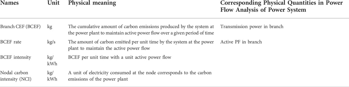
TABLE 1. THE basic physical quantities of CEF analysis.

For a power system with n_B nodes and n_G generators, without considering the active power loss, the NCI calculation formula is as follows:

${\mathit{E}}_{\mathrm{N}}={\left({\mathit{P}}_{\mathrm{N}}-{\mathit{P}}_{\mathrm{B}}^{\mathrm{T}}\right)}^{-1}{\mathit{P}}_{\mathrm{G}}^{\mathrm{T}}{\mathit{E}}_{\mathrm{G}}(1)$

where E_N is a n_B-dimensional NCI vector; P_N is the active power flux matrix of n_B nodes, which is a n_B-order diagonal matrix and the diagonal elements are the amount of active power flowing through each node; P_B is the branch PF distribution matrix. If there is at least one straight-through branch (transmission line) between nodes i and j (i, j = 1, 2, ..., n_B) and the quantity of active PF from this branch (or branches) is $p$, then P_Bij = p and P_Bji = 0. Otherwise P_Bij = P_Bji = 0; P_G is the power injection distribution matrix of size n_G × n_B. If the kth generator is connected to the node j, and the power injected from the kth generator to node j is p, then P_Gkj = p; E_G is a n_G-dimensional generator carbon emission intensity (CEI) vector, where the kth element represents the CEI of the kth generator set.

The isolated nodes should not be included in the matrix calculation in this study in order to avoid the singular matrix. A network’s isolated node is defined as a node that is not adjacent to any other nodes.

Transmission loss allocation method based on the active power flow tracking

The power grid model is considered a lossless network in the preceding CEF calculation. In the actual power grid, however, this analysis method will cause errors. As a result, the existing lossy network should be converted to an equivalent lossless network. There is no doubt that electricity consumption is the root cause of electricity production, so consumers and producers should share network loss.

Based on the power flow tracking method in the power system (Power, 2017), this paper employs a network lossless equivalent method combining downstream tracking and upstream tracking. The network loss is proportional to the additional load at nodes based on the original load amount. The network loss is equivalent to the extra load at generation nodes based on the power injected by the generator.

According to upstream tracking, let P^(g) be the active power flux vector of each node in the equivalent lossless network. P_GN is the n_B-dimensional vector that describes the active power output of generators received by each node. By introducing an upstream distribution matrix A_u, the power balance expression of each node can be written as follows:

${\mathit{A}}_{\mathit{u}}{\mathit{P}}^{\left(g\right)}={\mathit{P}}_{GN}(2)$

${\left[{\mathit{A}}_{\mathit{u}}\right]}_{ij}=\{\begin{array}{cc}1,& i=j\\ -\left|P_{j-i}\right|/P_j,& j\in U_i\\ 0,& others\end{array}(3)$

where U_i is the set of upstream nodes of node i.

Since the network loss is relatively low, it can be assumed that the proportion of load in the active power flux of the node remains unchanged before and after the equivalence; hence, the equivalent load at node i is

$\left|P_{Li}^{\left(g\right)}\right|=\frac{\left|P_{Li}^{\left(g\right)}\right|}{P_i^{\left(g\right)}}{P}_i^{\left(g\right)}\cong \frac{P_{Li}}{P_i}{P}_i^{\left(g\right)}(4)$

The network loss equivalent to the load node is

$\Delta {\mathit{P}}_L={\mathit{P}}_L^{\left(g\right)}-{\mathit{P}}_L(5)$

where P_L^(g) is the equivalent nodal load vector, P_L is the nodal load vector before equivalence.

The process of equivalent network loss to the generation node by the downstream tracking method is similar to the above process. By introducing a downstream distribution matrix A_d, the power balance expression of each node can be written as follows:

${\mathit{A}}_{\mathit{d}}{{\mathit{P}}^{\left(g\right)}}^{\prime }={\mathit{P}}_L(6)$

${\left[{\mathit{A}}_{\mathit{d}}\right]}_{ij}=\{\begin{array}{cc}1,& i=j\\ -\left|P_{i-j}\right|/P_j,& j\in D_i\\ 0,& others\end{array}(7)$

where D_i is the set of downstream nodes of node i.

Further, elements of the vector P_GN after equivalence is

$\left|P_{GNi}^{\left(g\right)}\right|=\frac{\left|P_{GNi}^{\left(g\right)}\right|}{P_i^{\left(g\right)}}{P}_i^{\left(g\right)}\cong \frac{P_{GNi}}{P_i}{P}_i^{\left(g\right)}(8)$

The network loss equivalent to the generation node is

$\Delta {\mathit{P}}_G={\mathit{P}}_{GN}-{\mathit{P}}_{GN}^{\left(g\right)}(9)$

The total network loss in the system is

$Loss=\Delta {\mathit{P}}_L=\Delta {\mathit{P}}_G(10)$

As stated previously, both the generation side and the load side should share the transmission network loss. Consequently, the allocation ratio β∈(0, 1) is set to allocate a portion β of the total network loss to the generation side and a portion 1 − β to the load side, which can be expressed as follows:

$\Delta {\mathit{P}}_G^{\prime }=\beta \Delta {\mathit{P}}_G(11)$

$\Delta {\mathit{P}}_L^{\prime }=\left(1-\beta \right)\Delta {\mathit{P}}_L(12)$

The allocation ratio β can be negotiated by power generation companies, electricity consumers and electricity retailers.

Problem formulation of power system optimal carbon emission flow

The CEFL of the network loss apportioned to the generation side can be directly calculated by multiplying the apportioned network loss by the generator’s CEI. By analyzing the distribution characteristics of CEF in the power grid, the CEFL assigned to the load side can be determined.

The equivalent network loss of the load side can be related to the generator through the path of active power transmission by introducing the generator-to-node incidence matrix R_U-N. R_U-N can be calculated as follows:

$R_{U-N}={\left[P_N{\left(P_N-P_B^T\right)}^{-1}{P}_G^T\right]}^T(13)$

The size of the R_U-N is K×N. After elements in R_U-N are normalized by the sum of all elements in the column, the element‾R_U-Nij in‾R_U-N represents the percentage of active power contribution of the ith generator to the load on node j. Further, the load side equivalent network loss traced to each generator can be calculated by the following formula:

$\Delta P_{G-L}={\left(diag\left(\Delta P_L^{\prime }\right){\overline{R}}_{U-N}\right)}^T(14)$

ΔP_G-L is a matrix of size K × N, where the element ΔP_G-Lij represents the part of the network loss shared by node j from the i_th generator. Each row of the matrix is summed to obtain the n_G-dimensional vectorΔP_g-l. The element ΔP_g-li in this vector represents the active power contributed by the ith generator to the network loss allocated to all its associated nodes.

Finally, the total CEL F_CEFL in the power system can be calculated by the following formula:]

$F_{CEFL}=E_G^T\left(\Delta {\mathbf{P}}_G^{\prime }+\Delta {\mathbf{P}}_{g-l}\right)(15)$

Based on the OPF problem, the OCEF problem is constructed by adding the objective of reducing unnecessary CEFL. The construction of the OCEF in the power system can be stated as follows:

$\min .C_G+F_{CEFL}(16)$

Subject to:

$P_{gk}^{\min }\le P_{gk}\le P_{gk}^{\max },\forall k\in G(17)$

$Q_{gk}^{\min }\le Q_{gk}\le Q_{gk}^{\max },\forall k\in G(18)$

$V_k^{\min }\le \left|V_k\right|\le V_k^{\max },\forall k\in N_b(19)$

$\left|S_{lm}\right|\le S_{lm}^{\max },\forall \left(l,m\right)\in L(20)$

$P_{gk}-P_{dk}={\displaystyle \sum }_{l\in N_b\left(k\right)}\mathrm{R}\mathrm{e}\left\{V_k\left(V_k^{\ast }-V_l^{\ast }\right){\mathrm{y}}_{kl}^{\ast }\right\}(21)$

$Q_{gk}-Q_{dk}={\displaystyle \sum }_{l\in N_b\left(k\right)}\mathrm{I}\mathrm{m}\left\{V_k\left(V_k^{\ast }-V_l^{\ast }\right){\mathrm{y}}_{kl}^{\ast }\right\}(22)$

where G is a set composed of all generators in the system; P_gk is the active output of the kth generator; Q_gk is the reactive output of the kth generator; V_k is the voltage phasor of node k; N_b is the set composed of all nodes in the system; S_lm is the power transmitted on the branch l-m; L is the set of nodes connected by a transmission line. (21) and (22) describe the system power balance constraint.

Proximal policy optimization algorithm

This paper employs the PPO algorithm, which is effective, robust and generalizable. The PPO algorithm and the TRPO algorithm have essentially the same structure, both utilizing the policy gradient method for training, i.e., parameterising the strategy. The strategy is optimized by designing an objective function to measure the quality of the strategy and then maximizing this objective function using the gradient ascent method.

The objective function of PPO can be expressed as follows:

$\underset{\theta }{\max }J\left(\theta \right)={\mathrm{E}}_{s_0}\left[V^{{\pi }_{\theta }}\left(s_0\right)\right]={\mathrm{E}}_{{\pi }_{\theta }}\left[{\displaystyle \sum }_{t=0}^{\infty }{\gamma }^{t}r\left({\mathit{s}}_t,{\mathit{a}}_t\right)\right](23)$

where θ is the parameter of random strategy π_θ; π_θ is the probability function modelled by neural networks, which input is a certain state, and the output is the probability distribution of taking action in this state; s_t is the state at tth step; a_t is the action at tth step; γ is the discount coefficient; r (s_t, a_t) is the return function; V^πθ(•) is the value function under the strategy π_θ.

The following formula calculates the gap between the objective functions under the old and new strategies:

$\begin{array}{c}J\left({\theta }^{\prime }\right)-J\left(\theta \right)={\mathrm{E}}_{{\pi }_{{\theta }^{\prime }}}\left[{\displaystyle \sum }_{t=0}^{\infty }{\gamma }^t\left[r\left(s_t,a_t\right)+\gamma V^{{\pi }_{\theta }}\left(s_{t+1}\right)-V^{{\pi }_{\theta }}\left(s_t\right)\right]\right]\end{array}(24)$

By introducing the advantage function A^πθ(s_t, a_t), (Eq. 24) can be rewritten as follows:

$J\left({\theta }^{\prime }\right)-J\left(\theta \right)==\frac{1}{1-\gamma }{\mathrm{E}}_{s\sim v^{{\pi }_{{\theta }^{\prime }}}}{\mathrm{E}}_{\mathit{a}\sim {\pi }_{{\theta }^{\prime }}\left(\cdot |s\right)}\left[A^{{\pi }_{\theta }}\left(\mathit{s},\mathit{a}\right)\right](25)$

The advantage function can be calculated by generalized advantage estimation (GAE) (Schulman et al., 2018):

$A^{{\pi }_{\theta }}\left({\mathit{s}}_t,{\mathit{a}}_t\right)={\displaystyle \sum }_{l=0}^{\infty }{\left(\gamma \lambda \right)}^l\left(r_t+\gamma V^{{\pi }_{\theta }}\left(s_{t+1}\right)-V^{{\pi }_{\theta }}\left(s_t\right)\right)(26)$

where λ∈[0, 1] is the hyperparameter defined for computing the generalized advantage estimation.

Therefore, it is only necessary to find a new policy to let ${\mathrm{E}}_{s\sim v^{{\pi }_{\theta {}^{\prime }}}}{\mathrm{E}}_{\mathit{a}\sim {\pi }_{\theta {}^{\prime }}\left(\cdot |s\right)}\left[A^{{\pi }_{\theta }}\left(\mathit{s},\mathit{a}\right)\right]$, so that the monotonically increasing performance of the policy can be guaranteed.

Since the new strategy is unknown and must also be used for sampling, it is extremely challenging to solve the equation directly. Hence, if the change in state visit distribution between two policies is ignored and the old strategy’s state distribution is adopted directly, after introducing importance sampling to process distribution of action, the optimization goal can be defined as:

$L_{\theta }\left({\theta }^{\prime }\right)=J\left(\theta \right)+\frac{1}{1-\gamma }{\mathrm{E}}_{s\sim v^{{\pi }_{\theta }}}{\mathrm{E}}_{\mathit{a}\sim {\pi }_{\theta }\left(\cdot |s\right)}\left[R\left(\theta \right)A^{{\pi }_{\theta }}\left(\mathit{s},\mathit{a}\right)\right](27)$

where the importance sampling is

$R\left(\theta \right)=\frac{{\pi }_{{\theta }^{\prime }}\left(\mathit{a}|\mathit{s}\right)}{{\pi }_{\theta }\left(\mathit{a}|\mathit{s}\right)}(28)$

PPO algorithm uses truncation to limit Kullback-Leibler (KL) divergence (Kullback and Leibler, 1951) between old and new policies, ensuring they are close enough and avoiding complex constrained problems. The objective function of optimization can be rewritten as follows:

$\mathrm{a}\mathrm{r}\mathrm{g}\underset{{\theta }^{\prime }}{\max }{\mathrm{E}}_{s\sim v^{{\pi }_{{\theta }_k}}}{\mathrm{E}}_{a\sim {\pi }_{{\theta }_k}\left(\cdot |s\right)}\left[\min \left(R\left(\theta \right)A^{{\pi }_{{\theta }_k}}\left(\mathit{s},\mathit{a}\right),\mathrm{c}\mathrm{l}\mathrm{i}\mathrm{p}\left(R\left(\theta \right),1-ϵ,1+ϵ\right)A^{{\pi }_{{\theta }_k}}\left(\mathit{s},\mathit{a}\right)\right)\right](29)$

where, clip (x, l, r) = max (min (x, r), l) restricts x within $\left[l,r\right]$; $ϵ$ is the hyperparameter to adjust the truncation range.

Proposed DRL-based OCEF solutions

The framework for handling the OCEF problem of the power system using the DRL-based solver proposed in this paper is depicted in Figure 1. The PPO agent is trained by interacting with a simulated power grid environment to discover the optimal strategy for various grid states. When constructing the OCEF solver with a well-trained agent, only forward propagation calculations are required to obtain the (approximate) OCEF in the current state.

FIGURE 1

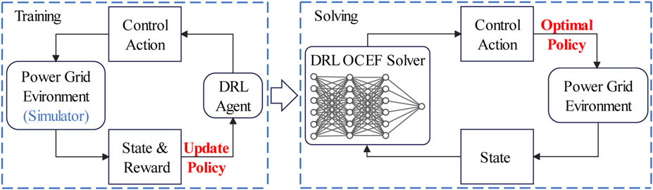
FIGURE 1. The DRL-based framework to solve the OCEF problem.

State and action space

The agent receives the state variables provided by the simulated grid environment and then outputs corresponding actions to modify the current state of the grid in order to reduce power generation cost and CEFL. Therefore, the state should contain the key variables describing the grid’s current state, which the agent can use to output the optimal action.

The state space and action space construction method used in this paper refer to (Zhou et al., 2021). The key variables to describe the power grid state are: active load P_d and reactive load Q_d of n_B nodes; amplitude |Y| and phase angle ∠Y of self-admittance of n_B nodes; the active power output P_g and the voltage V_g of the n_G generators. Thus, the state space is shown as follows:

$\begin{array}{cc}state=& [P_{d1}\sim P_{d{n}_B},Q_{d1}\sim Q_{d{n}_B},\left|Y_1\right|\sim \left|Y_{n_B}\right|,\\ & \angle Y_1\sim \angle Y_{n_B},P_{g1}\sim P_{g{n}_G},V_{g1}\sim V_{g{n}_G}]\end{array}(30)$

The action space, which contains active power output of generator adjustment value ΔP_g and voltage adjustment ΔV_g of n_G generators, is shown in the Formula 31:

$action=\left[\Delta P_{g1}\sim \Delta P_{g{n}_G},\Delta V_{g1}\sim \Delta V_{g{n}_G}\right](31)$

The structure of policy network and value network

PPO utilizes two neural networks to fit the policy function and the value function, similar to the Actor-Critic algorithm. The policy network, which is the agent in the PPO algorithm, is responsible for generating actions according to the state. The value network generates the appropriate value based on the present state.

First, the primary portion of the policy network is constructed. Considering the power grid’s topology, this paper divides the six state variables in the state space into generator state variable matrix sg of size 2×n_G and node state matrix sb of size 4×n_B. Two convolutional layers are required to extract the matrices’ information when two sets of state variable matrices are input into the policy network. There are 16 convolutional kernels of size 3 × 3 and a stride size of 1 × 1 for each of the two convolutional layers, whose parameters are identical. Using zero padding to fill the edges of the matrix guarantees that all state variable information will be sensed. Unlike a convolutional neural network that processes image input, this paper does not use max-pooling to extract features from the convolutional layer’s output to preserve all power grid state parameters.

Second, the policy network is designed to generate actions in a particular way. PPO is a typical DRL algorithm with stochastic strategies. For discrete actions, the agent will directly generate the probability distribution of each action and make specific action decisions by random sampling based on the probability distribution generated for training. When the agent is used as a solver, it will always select the action with the highest probability and thus make the optimal decision. For continuous action in this paper, the agent generates the Gaussian distribution’s mean and variance, which have the same degree of freedom of action. During training, the agent randomly sampled specific actions based on the Gaussian distribution. As a solver, it always selects the mean action value because the mean value is the action value with the maximum probability.

Third, select the activation function and construct the remaining policy network components. The policy network in this paper consists of two output layers. Using the Tanh function to activate the outputs will generate actionable means. The parameterization is used for variation to make the parameters trainable. The fully connected layer constructs all hidden layers in the policy network, and the layer norm is used to avoid the gradient vanishing problem. Figure 2 is a diagram illustrating the structure of the policy network.

FIGURE 2

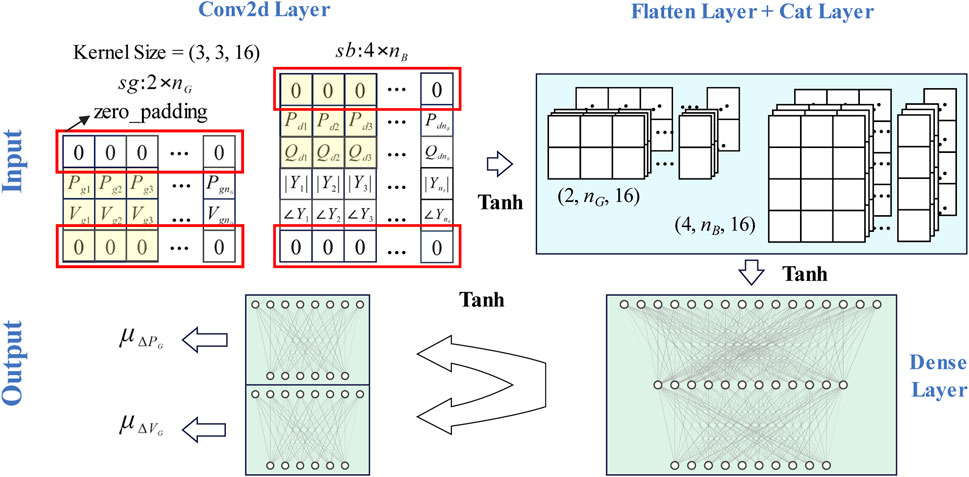
FIGURE 2. Network structure.

The structure of the value network is comparable to that of the policy network, as its output is the value determined based on the current state. The size of the output layer only needs to be as large as the output value, so no additional details are required.

The hyper-parameters of the policy network and the value network are shown in Table 2.

TABLE 2

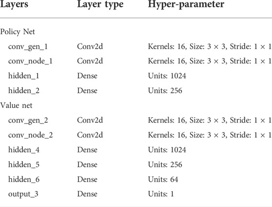
TABLE 2. The hyperparameters of the policy network and the value network.

The trainable parameters of the neural networks in both the policy network and the value network should be initialized with orthogonal initialization. The orthogonal initialization can further mitigate the problems of gradient disappearance and gradient explosion that can occur during the training process, thereby enhancing the training’s stability.

Training process of PPO agents

In the DRL algorithm, agents gain experience by constantly interacting with the environment and ultimately acquire the optimal strategy to guide them to obtain the greatest cumulative reward. This study uses a PF solver to simulate the power grid environment. Figure 3 is The flowchart of the agent interacting with the simulated power grid environment.

FIGURE 3

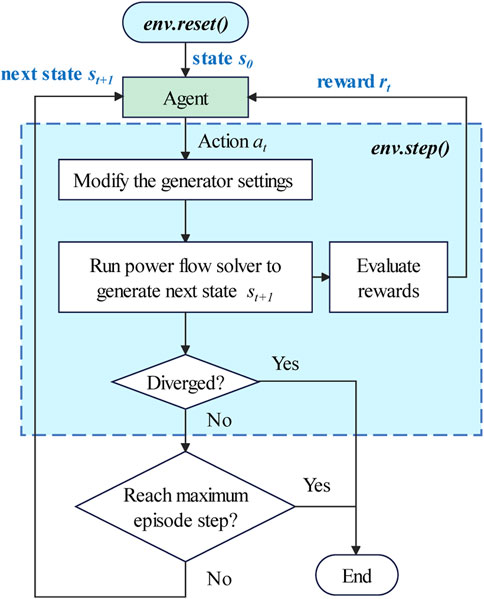
FIGURE 3. The flowchart of the agent interacting with the simulated power grid environment.

In this process, the initial state s₀=(sg₀, sb₀) is randomly generated by the function env. reset() according to the actual topology of the power grid. It is necessary to ensure that the system’s initial state satisfies the operational constraints. At tth step, the agent detects the state s_t of the system from the simulated power grid environment, modifies the current state based on the action a_t specified by the strategy, and obtains the next state s_t+1. Additionally, the environment provides the agent with an immediate reward r_t for taking action a_t state s_t and a signal done indicating whether the termination state has been reached. The interaction process between the agent and the environment will continue until it is terminated. The above environment is defined as the function env. step().

The immediate reward value for the current step is calculated according to (32), which is a piecewise function. When the PF solver in the environment diverges, the environment will feed back a large negative reward to the agent, causing the agent to avoid this situation in the future. If some constraints are not met, the agent will receive a negative reward proportional to the overlimit value of various variables. Agents will make fewer decisions that may lead to constraint violations if the reward is low. When the PF solver is solvable, and there are no violation issues, the environment will give the appropriate reward based on the power generation cost and CEFL calculated from the current state. Agents will be encouraged to make decisions that reduce the cost of power generation and the CEFL by monetary incentives.

$reward=\{\begin{array}{cc}-5000,& \mathrm{i}\mathrm{f}\mathrm{P}\mathrm{F}\mathrm{s}\mathrm{o}\mathrm{l}\mathrm{v}\mathrm{e}\mathrm{r}\mathrm{i}\mathrm{s}\mathrm{d}\mathrm{i}\mathrm{v}\mathrm{e}\mathrm{r}\mathrm{g}\mathrm{e}\mathrm{d}\\ R_{Pg\_v}+R_{V\_v}+R_{Br\_v},& \mathrm{i}\mathrm{f}\mathrm{t}\mathrm{h}\mathrm{e}\mathrm{r}\mathrm{e}\mathrm{a}\mathrm{r}\mathrm{e}\mathrm{c}\mathrm{o}\mathrm{n}\mathrm{s}\mathrm{t}\mathrm{r}\mathrm{a}\mathrm{i}\mathrm{n}\mathrm{t}\mathrm{s}\mathrm{v}\mathrm{i}\mathrm{o}\mathrm{l}\mathrm{a}\mathrm{t}\mathrm{i}\mathrm{o}\mathrm{n}\mathrm{s}\\ 2000-{\mathrm{C}}_G-1000\times F_{CEFL}& \mathrm{i}\mathrm{f}\mathrm{f}\mathrm{e}\mathrm{a}\mathrm{s}\mathrm{i}\mathrm{b}\mathrm{l}\mathrm{e}\end{array}(32)$

where R_{Pg_v} is the negative of the overlimit value of the active power output of generators; R_{V_v} is the negative of the overlimit value of nodes voltage; R_{Br_v} is the negative of the overlimit value of the power transmitted by the line. To calculate the positive reward, the coefficient of the CEFL value F_CEFL is set to be the same order of magnitude as the generation cost.

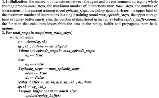
Although PPO belongs to the off-policy DRL algorithm, the interaction process can still utilize the replay buffer to save data. When the amount of data in the replay buffer reaches a predetermined threshold, the policy network and value network loss functions are calculated for propagation. At the beginning of the next interactive round, the data stored during the previous training round is cleared after the network parameters have been updated.

The loss function of the policy network is

$L_{A\mathrm{c}tor}=-\min \left(R{\left(\theta \right)}_t{A}^{{\pi }_{\theta }}\left(s_t,a_t\right),\mathrm{c}\mathrm{l}\mathrm{i}\mathrm{p}\left(R{\left(\theta \right)}_t,1-ϵ,1+ϵ\right)A^{{\pi }_{\theta }}\left(s_t,a_t\right)\right)-\alpha H\left({\pi }_{\theta }\left(•|s_t\right)\right)(33)$

where α is the regularization coefficient; H (π_θ(•|s_t)) is the entropy of the current strategy. In information theory and probability statistics, entropy is used as a measure to describe the uncertainty of random variables. The greater the entropy, the more average the probability of each action selected by a strategy. H (π_θ(•|s_t)) is calculated as follows:

$H\left({\pi }_{\theta }\left(•|s_t\right)\right)=E_{a_t\sim {\pi }_{\theta }}\left[-\log \left(\pi \left(a_t|s_t\right)\right)\right](34)$

The loss function of the value network is the advantage function obtained by GAE:

$L_{Critic}={\widehat{A}}_t^{GAE\left(\gamma ,\lambda \right)}={\displaystyle \sum }_{l=0}^{\infty }{\left(\gamma \lambda \right)}^l{\delta }_{t+l}^V(35)$

Algorithm 1 shows in detail the training process of the PPO agent to solve the OCEF.

Algorithm 1. PPO training for solving the OCEF problem.

Case study

The proposed method for solving the OCEF problem based on the DRL algorithm is tested on the IEEE-30 system. The system consists of six generators, 30 nodes and 41 lines. Python 3.7 and Pytorch 1.11.0 + cu113 are used to build a simulation test platform. The power grid simulation environment is built with the PF solver in Pypower. Pypower is a Python platform port to the Matpower toolkit in Matlab.

The default initial grid parameters of the IEEE-30 system are as follows. The outputs of the generator and load on the node are shown in Table 3.

TABLE 3

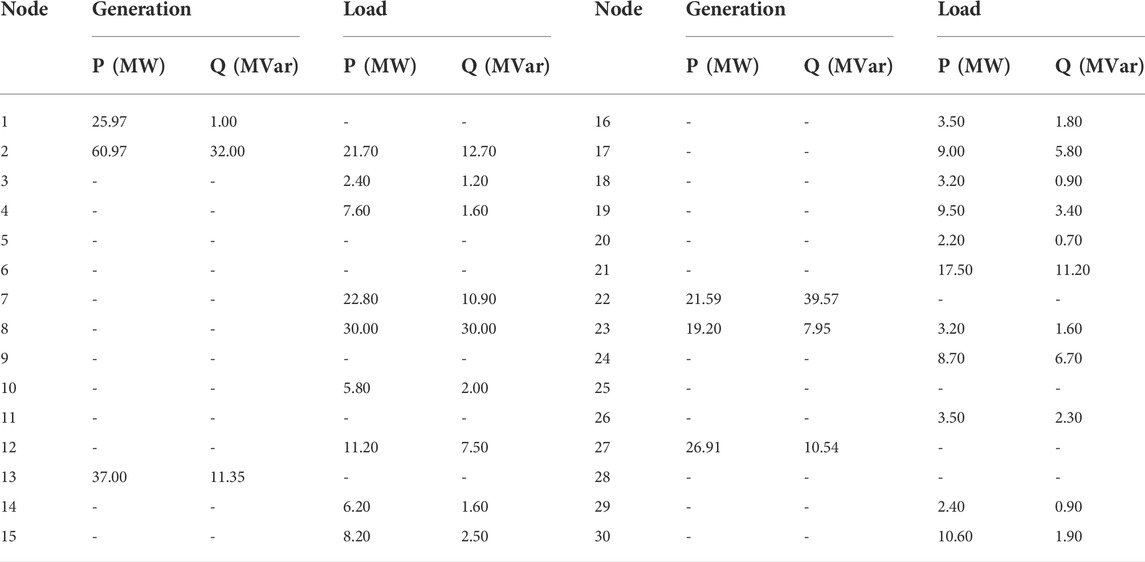
TABLE 3. The initial grid parameters of the IEEE-30 system.

The power transmitted on each branch is shown in Table 4.

TABLE 4

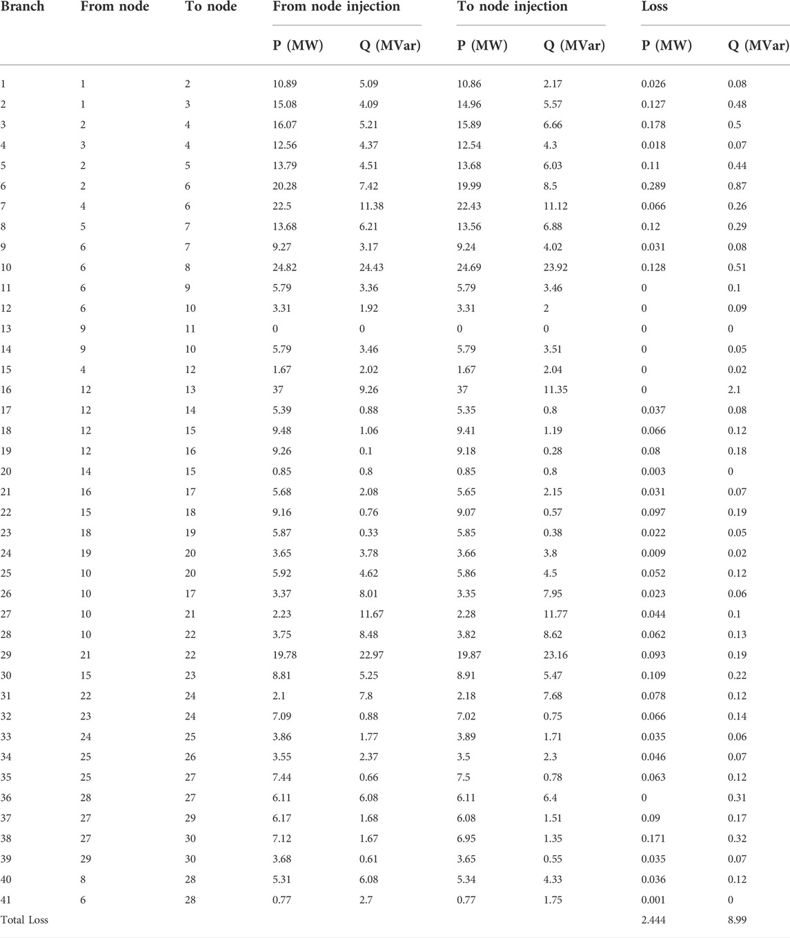
TABLE 4. The power transmitted on each branch.

The cost of generation is calculated as follows.

$C_G={\displaystyle \sum }_{k=1}^6{c}_2{P}_{gk}^2+c_1{P}_{gk}+c_0(36)$

The settings of the coefficient of each generator are shown in Table 5:

TABLE 5

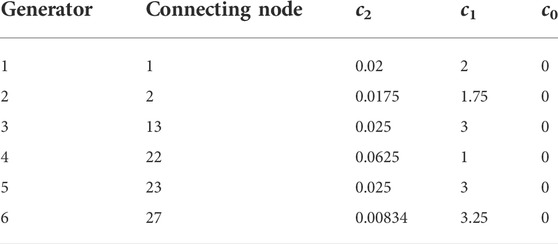
TABLE 5. The settings of the coefficient of each generator.

In order to conduct CEF analysis, this paper sets the CEI vector of each generator set as shown below:

$E_G={\left[\mathrm{0.52,0.15,0.38,0.52,0.16,0.28}\right]}^T(37)$

Tracking and allocation of CEFL

When the network loss is ignored, the calculation results of CEI and active flux of each node are shown in Table 6:

TABLE 6

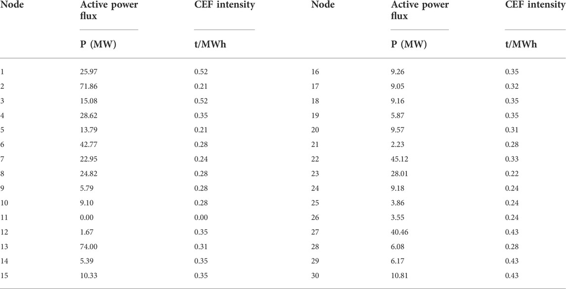
TABLE 6. The calculation results of CEI and active flux.

In this paper, the allocation ratio β is set to 0.5. The comparison of active power output and active load data of the generator before and after the allocation is as the Table 7 shows:

TABLE 7

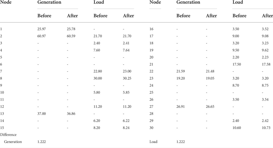
TABLE 7. The comparison of active power output and active load data.

It can be seen that, after allocation, the network loss caused by branch impedance is divided proportionally between the generation side and the load side. After tracing the CEFL, the results are shown in Table 8.

TABLE 8

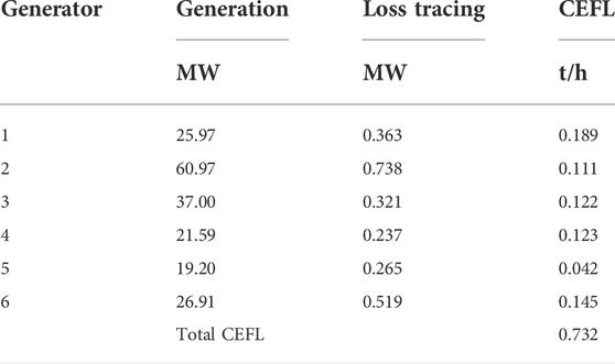
TABLE 8. The comparison of active power output and active load data.

Training process of DRL-Based OCEF solver

The initialization of the power system simulation environment includes two parts: load and generator random initialization and PF initialization. By sampling in the uniform distribution, the active and reactive loads are randomly generated between [0.6, 1.4]p.u.. In the IEEE-30 system, node 1, where generator one resides, is the balance node, and nodes where the other five generators reside are PV nodes. The generated load is randomly distributed to all six generators. After the generator output’s initialization, the generator’s voltage is randomly generated between [V_gmin, V_gmax]. The PF solver in Pypower is used to calculate the AC PF under the current network state, and the initial state s_g0 of the generator and the initial state s_b0 of the node are obtained, completing simulation environment state initialization.

The hyperparameter settings involved in Algorithm 1 are shown in Table 9:

TABLE 9

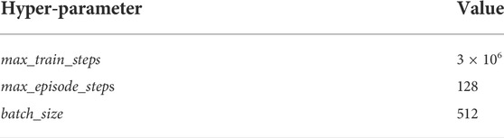
TABLE 9. The hyperparameter settings involved in Algorithm 1.

Table 10 shows the setting methods and meanings of hyperparameters involved in PPO algorithm.

TABLE 10

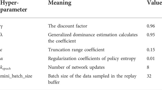
TABLE 10. Settings of the hyperparameters of the PPO algorithm.

After the replay buffer stores enough data, the mini_batch_size group of samples are randomly selected from the replay buffer to calculate the gradient of the policy network and the value network and update the network. The above sampling and update process will be performed k_epoch times when each replay buffer is full.

For the hyperparameters in the training process of policy network and value network, this paper sets them as follows: 1) set the initial value of the learning rate as 3 × 10^–4 and adopt the learning rate decay method, which makes the learning rate linearly decreases to 0 with the number of training steps; 2) in gradient backpropagation, gradient truncation is adopted to limit the parameters’ update range, and the truncation range is set as [-0.5, 0.5]. The above two hyperparameter settings will speed up network training and make the training process more stable.

In addition, this paper also takes the following measures to improve the training process: 1) standardize the advantage function; 2) standardize the input state variables into the network, and save the mean and variance of the state variables, so that the agent can standardize the input variables when it is called as the OCEF solver; 3) smooth the output of reward by using the reward scaling method proposed in (Engstrom et al., 2020); 4) refer to the Open AI Baseline (Baselines, 2022) example and set the parameter eps in the Adam optimizer to 1 × 10^–5 (default value is 1 × 10^–8).

After configuring the aforementioned parameters, Figure 4 and Figure 5 illustrate the agent training process. Figure 4 depicts the immediate reward curve after each agent-environment interaction during the training process. Figure 5 depicts the agent’s average reward for solving the target problem multiple times during the current training round, once every 512 steps. The difference between the two curves is that the curve in Figure 4 represents the outcome of the agent’s interaction with the environment using random strategies during the training process, whereas the curve in Figure 5 represents the agent’s adoption of the action value with the highest probability to interact with the environment, which is a deterministic strategy.

FIGURE 4

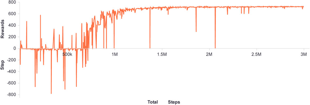
FIGURE 4. The rewards of evert step.

FIGURE 5

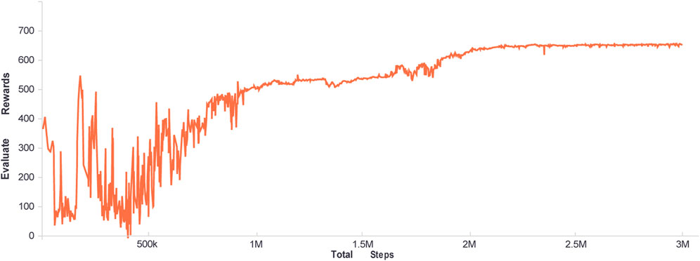
FIGURE 5. The average rewards of every evaluation.

As shown by the curve in Figure 4, during the first one million training steps, the agent made numerous random attempts and then began to find an effective way to obtain greater rewards. The curve can also show this process in Figure 5. With the agent’s exploration, within one million to two million steps, the agent can obtain stable good immediate rewards. The fluctuation curve in both figures indicates that the agent will continue to explore. Currently, as a result of the ongoing optimization of the strategy, the curve in Figure 5 is also gradually increasing. After two million steps, the agent’s strategy is effective and stable.

The verification of solution effect

To evaluate the effectiveness of the DRL-based solver proposed in this paper, the generator dispatching outcomes of OCEF and OPF are compared. Simultaneously, NSGA-II (Deb et al., 2002) with a population of 100 is utilized to solve OCEF, compared to the proposed method to validate its performance.

The generator dispatching results under OCEF obtained by the proposed solver are compared to the dispatching results under OPF to determine whether the results under OCEF can effectively balance the two objectives. When the OPF solver of Pypower (based on the interior point method) is utilized for dispatching optimization considering only the generator cost, Table 11 displays the active power output of each generator, the generation cost, and the tracked CEFL.

TABLE 11

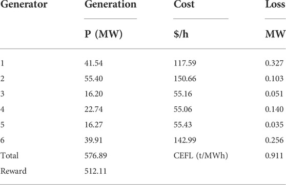
TABLE 11. The dispatching results OF OPF.

Table 12 displays the generator dispatching results when the DRL-based OCEF solver is invoked.

TABLE 12

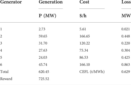
TABLE 12. The dispatching results of DRL-based OCEF.

It is evident that the DRL-based solver can achieve a balance between the two objectives, which raises the overall cost of power generation by 7.55% but reduces carbon flow loss by 30.95%.

Figure 6 illustrates the performance of the proposed method and NSGA-II in solving the problem with 10,000 random initial states. The graph on the left compares the amount of time required to solve a problem when both approaches yield the same result. The figure on the right compares the benefits of the two methods for simultaneously solving 10,000 identical problems. In terms of score and solution time, it can be seen that the method proposed in this paper is superior to NSGA-II. The DRL-based OCEF solver has a relatively stable effect on problems with varying initial conditions.

FIGURE 6

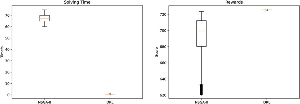
FIGURE 6. The performance comparison.

Figure 7 compares the solution processes of the DRL-based solver and NSGA-II when applied to the same problem. DRL solver does not need an iterative solving process, but adopts the optimal strategy to make decisions and achieves a good solution in several steps. In contrast, NSGA-II requires constant iteration, resulting in a higher computational cost and a slower solution speed.

FIGURE 7

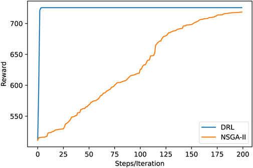
FIGURE 7. The comparison of solution processes.

Conclusion

In this paper, a DRL-based solver for multi-objective OCEF is presented and validated using a case study on the IEEE-30 system. In the case study, the DRL-based solver’s solution results are compared to those of NSGA-II. Experimental results indicate that the solution time of the proposed DRL-based OCEF solver is one-hundredth that of NSGA-II, and the solver’s performance is enhanced by at least 10 percent. In addition, the DRL-based solver is more stable and can satisfy real-time power dispatching needs.

Following is a summary of future research ideas:

1) More intricate dispatching scenarios for power systems can be considered. For instance, constraints such as the N-1 safety constraint and the generator climbing constraint can be considered, thereby enhancing the practical applicability of the DRL-based solver.

2) The actual state parameters of the power system can be used as training data for the model. As demonstrated in the case study, training the agent requires a large amount of data, and each round of interaction requires a time cross-section of system state parameters. In practice, collecting such a vast amount of data is difficult. Consequently, data generation techniques such as the generative adversarial network can be used to provide the necessary training data for DRL agents.

3) Consider utilizing the multiagent method to solve the OCEF problem in the larger system. Even though the performance of the DRL-based solution is superior to that of the conventional solution, the larger system still entails a larger action space and state space. This increases the difficulty of calculating the immediate reward value of environmental feedback in a simulated power system and increases network training requirements. When the original large system is partitioned, a single agent is responsible for the dispatching solution of each partition, and multiple agents are combined to reduce training difficulty.

Data availability statement

The original contributions presented in the study are included in the article/supplementary material, further inquiries can be directed to the corresponding author.

Author contributions

PQ and QH contributed to the conception and design of the study. PQ and JY performed the analysis. PQ wrote the first draft of the manuscript. PQ, JY, QH, PS, and PK wrote sections of the manuscript. All authors contributed to manuscript revision, read, and approved the submitted version.

Funding

This work was supported by the Science and Technology Project of State Grid Corporation of China under grant to 5419-202040493A-0-0-00.

Conflict of interest

PS and PK were employed by the company State Grid Xinjiang Electric Power Co Ltd.

The remaining authors declare that the research was conducted in the absence of any commercial or financial relationships that could be construed as a potential conflict of interest.

Publisher’s note

All claims expressed in this article are solely those of the authors and do not necessarily represent those of their affiliated organizations, or those of the publisher, the editors and the reviewers. Any product that may be evaluated in this article, or claim that may be made by its manufacturer, is not guaranteed or endorsed by the publisher.

References

Alsaif, A. (2017). Challenges and benefits of integrating the renewable energy technologies into the AC power system grid. https://www.semanticscholar.org/paper/Challenges-and-Benefits-of-Integrating-the-Energy-Alsaif/22a08488e3859f490824bc2936f4abe058e9b545 (accessed August 5, 2022).

Google Scholar

Baselines (2022). Baselines. https://github.com/openai/baselines (accessed August 6, 2022).

Google Scholar

Bayindir, R., Demirbas, S., Irmak, E., Cetinkaya, U., Ova, A., and Yesil, M. (2016). “Effects of renewable energy sources on the power system,” in 2016 IEEE International Power Electronics and Motion Control Conference, 388–393. doi:10.1109/EPEPEMC.2016.7752029

CrossRef Full Text | Google Scholar

Bellman, R. (1957). A markovian decision process. Indiana Univ. Math. J. 6, 679–684. doi:10.1512/iumj.1957.6.56038

CrossRef Full Text | Google Scholar

Cao, H., Gao, C., He, X., Li, Y., and Yu, T. (2020). Multi-agent cooperation based reduced-dimension Q(λ) learning for optimal carbon-energy combined-flow. Energies 13, 4778. doi:10.3390/en13184778

CrossRef Full Text | Google Scholar

Chen, J., Alnowibet, K., Annuk, A., and Mohamed, M. A. (2021). An effective distributed approach based machine learning for energy negotiation in networked microgrids. Energy Strategy Rev. 38, 100760. doi:10.1016/j.esr.2021.100760

CrossRef Full Text | Google Scholar

Deb, K., Pratap, A., Agarwal, S., and Meyarivan, T. (2002). A fast and elitist multi-objective genetic algorithm: NSGA-II. IEEE Trans. Evol. Comput. 6, 182–197. doi:10.1109/4235.996017

CrossRef Full Text | Google Scholar

Dhople, S. (2017). “Control of low-inertia AC microgrids,” in 2017 51st Annual Conference on Information Sciences and Systems, 1–2. doi:10.1109/CISS.2017.7926115

CrossRef Full Text | Google Scholar

Engstrom, L., Ilyas, A., Santurkar, S., Tsipras, D., Janoos, F., Rudolph, L., and Madry, A. (2020). Implementation matters in deep policy gradients: A case study on PPO and TRPO. arXiv preprint. doi:10.48550/arXiv.2005.12729

CrossRef Full Text | Google Scholar

Gong, X., Dong, F., Mohamed, M. A., Awwad, E. M., Abdullah, H. M., and Ali, Z. M. (2020). Towards distributed based energy transaction in a clean smart island. J. Clean. Prod. 273, 122768. doi:10.1016/j.jclepro.2020.122768

CrossRef Full Text | Google Scholar

Han, R., Hu, Q., Guo, Z., Quan, X., Wu, Z., and Hu, R. (2022). Optimal allocation method of residential air-conditioners: Trade-off solutions between economic costs and aggregation reliability. IEEE Open J. Power Energy 9, 131–142. doi:10.1109/OAJPE.2022.3151493

CrossRef Full Text | Google Scholar

Holland, J. H. (1992). Adaptation in natural and artificial systems: An introductory analysis with applications to biology, control, and artificial intelligence. Cambridge, Massachusetts, United States: MIT Press.

Google Scholar

Impram, S., Varbak Nese, S., and Oral, B. (2020). Challenges of renewable energy penetration on power system flexibility: A survey. Energy Strategy Rev. 31, 100539. doi:10.1016/j.esr.2020.100539

CrossRef Full Text | Google Scholar

Kaelbling, L. P., Littman, M. L., and Moore, A. W. (1996). Reinforcement learning: A survey. J. Artif. Intell. Res. 4, 237–285.

CrossRef Full Text | Google Scholar

Kang, C., Zhou, T., Chen, Q., Wang, J., Sun, Y., Xia, Q., et al. (2015). Carbon emission flow from generation to demand: A network-based model. IEEE Trans. Smart Grid 6, 2386–2394. doi:10.1109/TSG.2015.2388695

CrossRef Full Text | Google Scholar

Kang, C., Zhou, T., Chen, Q., Xu, Q., Xia, Q., and Ji, Z. (2012). Carbon emission flow in networks. Sci. Rep. 2, 479. doi:10.1038/srep00479

PubMed Abstract | CrossRef Full Text | Google Scholar

Kullback, S., and Leibler, R. A. (1951). On information and sufficiency. Ann. Math. Stat. 22, 79–86. doi:10.1214/aoms/1177729694

CrossRef Full Text | Google Scholar

Mnih, V., Kavukcuoglu, K., Silver, D., Graves, A., Antonoglou, I., Wierstra, D., and Riedmiller, M. (2013). Playing atari with deep reinforcement learning. arXiv preprint. doi:10.48550/arXiv.1312.5602

CrossRef Full Text | Google Scholar

Momoh, J. A., Adapa, R., and El-Hawary, M. E. (1999). A review of selected optimal power flow literature to 1993 I Nonlinear and quadratic programming approaches. IEEE Trans. Power Syst. 14, 96–104. doi:10.1109/59.744492

CrossRef Full Text | Google Scholar

Momoh, J. A., El-Hawary, M. E., and Adapa, R. (1999). A review of selected optimal power flow literature to 1993. II. Newton, linear programming and interior point methods. IEEE Trans. Power Syst. 14, 105–111. doi:10.1109/59.744495

CrossRef Full Text | Google Scholar

Papaefthymiou, G., and Dragoon, K. (2016). Towards 100% renewable energy systems: Uncapping power system flexibility. Energy Policy 92, 69–82. doi:10.1016/j.enpol.2016.01.025

CrossRef Full Text | Google Scholar

Power, K. Berg. (2017). Flow tracing: Methods and algorithms - implementation aspects. https://ntnuopen.ntnu.no/ntnu-xmlui/handle/11250/2452452 (accessed August 4, 2022).

Google Scholar

IEA, (2021). Executive summary - Renewables 2021 - Analysis. https://www.iea.org/reports/renewables-2021/executive-summary (Accessed August 5, 2022).

Google Scholar

Sang, L., Hu, Q., Xu, Y., and Wu, Z. (2022). Privacy-preserving hybrid cloud framework for real-time TCL-based demand response. IEEE Trans. Cloud Comput., 1–1. doi:10.1109/TCC.2022.3142009

CrossRef Full Text | Google Scholar

Schulman, J., Moritz, P., Levine, S., Jordan, M., and Abbeel, P. (2018). High-dimensional continuous control using generalized advantage estimation. arXiv preprint. doi:10.48550/arXiv.1506.02438

CrossRef Full Text | Google Scholar

Schulman, J., Wolski, F., Dhariwal, P., Radford, A., and Klimov, O. (2017). Proximal policy optimization algorithms. arXiv preprint. doi:10.48550/arXiv.1707.06347

CrossRef Full Text | Google Scholar

Seyam, S., Dincer, I., and Agelin-Chaab, M. (2020). Development of a clean power plant integrated with a solar farm for a sustainable community. Energy Convers. Manag. 225, 113434. doi:10.1016/j.enconman.2020.113434

CrossRef Full Text | Google Scholar

Sharma, R., Chandel, M. K., Delebarre, A., and Alappat, B. (2013). 200-MW chemical looping combustion based thermal power plant for clean power generation. Int. J. Energy Res. 37, 49–58. doi:10.1002/er.1882

CrossRef Full Text | Google Scholar

Sifat, N. S., and Haseli, Y. (2019). A critical review of CO2 capture technologies and prospects for clean power generation. Energies 12, 4143. doi:10.3390/en12214143

CrossRef Full Text | Google Scholar

van Otterlo, M., and Wiering, M. (2012). “Reinforcement learning and markov decision processes,” in Reinforcement learning: State-of-the-Art. Editors M. Wiering, and M. van Otterlo (Berlin, Heidelberg: Springer), 3–42. doi:10.1007/978-3-642-27645-3_1

CrossRef Full Text | Google Scholar

Zhan, Z.-H., Zhang, J., Li, Y., and Chung, H. S.-H. (2009). Adaptive particle swarm optimization. IEEE Trans. Syst. Man. Cybern. B 39, 1362–1381. doi:10.1109/TSMCB.2009.2015956

PubMed Abstract | CrossRef Full Text | Google Scholar

Zhang, W., Hu, Q., and Yu, X. (2022). Analysis on influence of residents’ response probability distribution on load aggregation effect. Front. Energy Res. 10. doi:10.3389/fenrg.2022.951618

CrossRef Full Text | Google Scholar

Zhang, X., Yu, T., Yang, B., Zheng, L., and Huang, L. (2015). Approximate ideal multi-objective solution Q(λ) learning for optimal carbon-energy combined-flow in multi-energy power systems. Energy Convers. Manag. 106, 543–556. doi:10.1016/j.enconman.2015.09.049

CrossRef Full Text | Google Scholar

Zhou, Y., Lee, W.-J., Diao, R., and Shi, D. (2021). Deep reinforcement learning based real-time AC optimal power flow considering uncertainties. J. Mod. Power Syst. Clean Energy, 1–11. doi:10.35833/MPCE.2020.000885

CrossRef Full Text | Google Scholar