The observability and controllability metrics of power system oscillations and the applications

1 Introduction

The concept of observability and controllability from modern control theory can assess systems, whether their internal states can be reflected by outputs and whether they can be affected by inputs (Angulo et al., 2020). However, a continuous indicator is needed to evaluate the observation and control performance under different measurement settings, system structures and parameter configurations. To provide quantitative information about the observability and controllability degree of a system, residue methods and geometric measures have been proposed (Heniche and Kamwa, 2002; Wang et al., 2017).

In recent years, the rapid development of renewable energy has brought more oscillation stability problems for power systems (Song and Blaabjerg, 2017; Xie et al., 2017; Li et al., 2020). The grid-connection of the renewable energy needs many electronic devices like converters, and these electronic devices together with their control system may form an equivalent “LC resonance circuit” with other parts of the power grid and generate oscillations. When the part of grid-connecting electronic system show “negative damping” at the oscillation frequency, the oscillation will diverge, and there will be oscillation stability problems.

Oscillation is a type of dynamic stability problem, and the modal analysis is one of the important methods. Since modal variables cannot be directly measured, accordingly, if the actual measured value can reflect the modal variable, the mode is assumed to be observable; if the control input can control the change of the modal variable, the mode is assumed to be controllable. So, the observability, controllability and relative methods are widely applied to power system oscillation study.

The residue method is often applied in input signals selection and controller parameters design in studying power system oscillation. Gallardo et al. (2017) and Oscullo and Gallardo (2020) used the residue method to find the best position of power system stabilizers to suppress electromechanical oscillations. The damping degradation degree and components that lead to the stability degradation can be estimated by calculating the residue under the open-loop state, providing the basis for controller design (DuFu and Wang, 2018). To achieve better adaptation in various operation conditions, the residue approach was applied to design the power oscillation damping controllers (Ping et al., 2014). By analyzing residue results under various working conditions, it is possible to determine the optimal position to insert the subsynchronous notch filter into the controller (Liu et al., 2017). The main drawback of the residue method is that only one oscillation eigenvalue is considered. The residue is a common quantitation indicator, but it is not suitable for comparing signals with different units.

The geometric measure first proposed aiming at the selection of the control loops permitting a good observability and controllability of system’s poles is defined based on the cosine of the angle between the left/right eigenvector and the input/output matrix of the system state space equation (Hamdan and Hamdan, 1987). It can be used with the advantage of normalization, but it cannot solve systems with repeated eigenvalues (Domínguez-García et al., 2014).

The method of participation factor in the power system can also reflect part of system observability and controllability degree (He et al., 2019; Huang et al., 2019; Lei et al., 2019; Zhou et al., 2019). To monitor oscillation, Lei et al. (2019) and Huang et al. (2019) respectively determined the type and locations of components causing oscillation by calculating the participation factor. To suppress oscillations, strong correlation variables were determined by the participation factor method, and then, a damping controller was designed (Zhou et al., 2019). Besides, the optimal parameter design of controllers can be determined by analyzing the participation factors of dominant modes (He et al., 2019). However, participation factor methods can only reflect the observability from state variables but not actual measurable values.

This paper proposes the novel observability metric and controllability metric from the perspective of modal analysis. We can use the concept of metric to quantify the observability and controllability to monitor and control oscillations. Modal observability metric (OM) represents the degree of reflection of monitoring point measurement on a power system mode. Controllability metric (CM) characterizes the performance of actuating point control input on a power system mode.

The main contributions are as follows: 1) the concepts of observability and controllability metrics for system with distinct and repeated eigenvalues are proposed from the viewpoint of oscillation modes, and it is proved mathematically that their effects can degenerate into residue and participation factors under certain conditions; 2) in order to compare control effect of different input signals and reflection degree of different output signals to different oscillation modes, the concepts of dominant mode observability ratio, dominant mode controllability ratio, oscillation mode comprehensive observability metric (MCOM) and mode comprehensive controllability metric (MCCM) are proposed. Compared with the residue method, geometric measures and participation factor, MCOM and MCCM can solve the global modal analysis (not only one eigenvalue at a time), applicable to systems with not only distinct but also repeated eigenvalues.

The rest of this paper is organized as follows: In Section 2, the concepts of observability metric and controllability metric are defined respectively, and from the perspective of controller design, Section 3 defines MCOM and MCCM. In Section 4, their meaning and advantages are analyzed. In Section 5, the theory is verified by the small-signal model and time-domain simulation. Finally, in Section 6 the conclusion is given.

2 Observability metric and controllability metric

In this section, the definition of observable ratio and controllable ratio are proposed to normalize units. And to comprehensively consider the relative observation and control effect of all the oscillation modes concerned, comprehensive observability metric and comprehensive controllability metric are defined. Before all these definitions, the controller characteristic requirements need to be analyzed.

2.1 System model and modal transformation

A general N_s-order system can be expressed in the form of state space in Eq. 1. Where X is the state variables matrix (N_s-order); u is the system input; Y is the system output; A, B and C matrixes are the system state, input and output coefficient matrixes, respectively.

$\{\begin{array}{c}\dot{\mathit{X}}=\mathit{A}\mathit{X}+\mathit{B}\mathit{u}\\ \mathit{Y}=\mathit{C}\mathit{X}\end{array}(1)$

It is assumed that N complex eigenvalues are obtained through analyzing the system coefficient matrix A (N≤N_S for the existing of real eigenvalues). And N₁ is set as the number of complex eigenvalues in various values.

When eigenvalues are all distinct (N₁ = N), the system can be completely decoupled by a linear transformation. It can be proved that the right eigenvector E exists to convert the state space expression of the system into Eq. 2.

$\{\begin{array}{c}\dot{\mathit{Z}}=\mathit{\Lambda }\mathit{Z}+{\mathit{F}}^T\mathit{B}\mathit{u}\\ \mathit{Y}=\mathit{C}\mathit{E}\mathit{Z}\end{array}(2)$

where Z is the transferred decoupled state variables matrix (or modal variables matrix); Λ is the eigenvalue diagonal matrix in Eq. 3, F is the left eigenvector matrix, satisfying E⁻¹ = F^T. Where, i is the number of complex eigenvalues in various values, i = 1 ∼ N₁.

$\mathit{\Lambda }=diag\left[\begin{array}{ccccc}{\lambda }_1& \cdots & {\lambda }_i& \cdots & {\lambda }_{N_1}\end{array}\right](3)$

For a more general case, i.e., if there are repeated eigenvalues (N>N₁), the coefficient matrix cannot be completely decoupled by a linear transformation. In the theory of linear systems (Pratzel-Wolters, 1982), Jordan canonical form is defined as the minimum coupling form that can be achieved. The transformation matrix Q exists to convert the state space expression of the system into Eq. 4, acting as an approximately right eigenvector.

$\{\begin{array}{c}\dot{\mathit{Z}}=\mathit{J}\mathit{Z}+{\mathit{L}}^T\mathit{B}\mathit{u}\\ \mathit{Y}=\mathit{C}\mathit{Q}\mathit{Z}\end{array}(4)$

where J is the Jordan canonical form matrix; L acts as an approximate left eigenvector matrix, satisfying Q⁻¹ = L^T. Let the ith different eigenvalue includes s_i repeated eigenvalues. Each eigenvalue λ_i corresponds to a set of modal variables Z_i(si×1), approximate right eigenvector q_i(N×si) and approximate left eigenvector l_i(N×si). Therefore, the coefficient matrix can be transformed into the form of Eq. 5.

$\mathit{J}=diag\left[\begin{array}{ccccc}{\mathit{J}}_1& \cdots & {\mathit{J}}_i& \cdots & {\mathit{J}}_{N_1}\end{array}\right](5)$

Similarly, the Jordan block corresponding to the ith distinct characteristic eigenvalue is J_i, and its dimension is s_i. The concrete form is related to the algebraic multiplicity and geometric multiplicity of Jordan block. In particular, when the algebraic multiplicity is equal to geometric multiplicity, the form of Jordan block is Eq. 6. When the two multiplicities are different, they may be related to strong resonance (Dobson et al., 2001). In this paper, we only study the cases satisfying Eq. 6, which may be caused by multiple machines.

${\mathit{J}}_i=\left[\begin{array}{cccc}{\lambda }_i& 1& & \\ & {\lambda }_i& \ddots & \\ & & \ddots & 1\\ & & & {\lambda }_i\end{array}\right](6)$

To more accurately characterize oscillation mode b∈(1,2…N₁/2), a pair of conjugate eigenvalues in the Λ or s_b pairs of conjugate eigenvalues in J are considered together. Each pair of conjugate eigenvalues describes the characteristics of the same mode, and s_b pairs of conjugate repeated eigenvalues describe the characteristics of s_b coupled modes with the same frequency. Consider the coupled modes together, we get oscillation modal variable matrix ${\stackrel{\sim }{\mathit{Z}}}_{b\left(2sb\times 1\right)}$.

The relevant information corresponding to mode b in the system with distinct or repeated eigenvalues is shown in Table 1, where, Λ_b(2×2), ${\stackrel{\sim }{\mathit{J}}}_{b\left(2sb\times 2sb\right)}$and ${\stackrel{\sim }{\mathit{Z}}}_{b\left(2sb\times 1\right)}$ are defined as Eqs. 7–9.

${\mathit{\Lambda }}_b=diag\left[\begin{array}{cc}{\lambda }_b& {\overline{\lambda }}_b\end{array}\right](7)$

${\stackrel{\sim }{\mathit{J}}}_b=diag\left[\begin{array}{cc}{\mathit{J}}_b& {\overline{\mathit{J}}}_b\end{array}\right](8)$

${\stackrel{\sim }{\mathit{Z}}}_b={\left[\begin{array}{cc}{\mathit{Z}}_b& {\overline{\mathit{Z}}}_b\end{array}\right]}^{\mathrm{T}}(9)$

TABLE 1

TABLE 1. Information corresponding to mode b.

2.2 Definition of observability metric

The degree of modal observability measures the ability of the output Y to reflect the mode of the system.

When eigenvalues are distinct, to reflect the observable degree of the oscillation mode, the system output Y is expressed as the sum of the modal components in Eq. 10.

$\mathit{Y}={\displaystyle \sum }_{b=1}^M\mathit{C}\left[\begin{array}{cc}{\mathit{e}}_b& {\overline{\mathit{e}}}_b\end{array}\right]{\stackrel{\sim }{\mathit{Z}}}_b(10)$

In Eq. 10, only M oscillation mode component terms are shown, corresponding to N₁ eigenvalues (N₁ = 2M). Eq. 10 indicates that the observable degree of the oscillation mode in the measured output Y can be represented by matrix $\mathit{C}\left[\begin{array}{cc}{\mathit{e}}_b& {\overline{\mathit{e}}}_b\end{array}\right]$. Therefore, the definition of the observability metric of oscillation mode b is proposed in Eq. 11.

$m_{ob}={\Vert \mathit{C}\left[\begin{array}{cc}{\mathit{e}}_b& {\overline{\mathit{e}}}_b\end{array}\right]\Vert }_F(11)$

where${\Vert \cdot \Vert }_F$is the Frobinus norm of the matrix. The observability metric m_ob can quantitatively reflect the observability degree of a system mode. Specifically, the larger m_ob is, the stronger the observability degree of the oscillation mode ${\stackrel{\sim }{\mathit{Z}}}_b$is in the output signal Y. This means the component of the oscillation mode can be better reflected in the output signal.

When the eigenvalues are repeated, Y is expressed in Eq. 12.

$\mathit{Y}={\displaystyle \sum }_{b=1}^M\mathit{C}\left[\begin{array}{cc}{\mathit{q}}_b& {\overline{\mathit{q}}}_b\end{array}\right]{\stackrel{\sim }{\mathit{Z}}}_b(12)$

In this case, the definition of OM is proposed in Eq. 13.

$m_{ob}={\Vert \mathit{C}\left[\begin{array}{cc}{\mathit{q}}_b& {\overline{\mathit{q}}}_b\end{array}\right]\Vert }_F(13)$

2.3 Definition of controllability metric

The controllability degree of the system measures the control ability of input u to the system modal variable Z.

When the eigenvalues are distinct, to reflect the controllability of oscillation modes, the variables in state equation are separated in Eq. 14, considering the input in Eq. 2.

${\dot{\mathit{Z}}}_i={\mathit{\Lambda }}_i{\mathit{Z}}_i+{\mathit{f}}_i^T\mathit{B}\mathit{u}(14)$

To more clearly express the properties of oscillation mode, Eq. 14 can be expressed as Eq. 15.

${\dot{\stackrel{\sim }{\mathit{Z}}}}_b={\mathit{\Lambda }}_b{\stackrel{\sim }{\mathit{Z}}}_b+{\left[\begin{array}{cc}{\mathit{f}}_b& {\overline{\mathit{f}}}_b\end{array}\right]}^T\mathit{B}\mathit{u}(15)$

Matrix ${\left[\begin{array}{cc}{\mathit{f}}_b& {\overline{\mathit{f}}}_b\end{array}\right]}^T\mathit{B}$ can characterize the controllability of input u to oscillation modal variable${\stackrel{\sim }{\mathit{Z}}}_b$, so the definition of controllability metric of oscillation mode b is proposed in Eq. 16.

$m_{cb}={\Vert {\left[\begin{array}{cc}{\mathit{f}}_b& {\overline{\mathit{f}}}_b\end{array}\right]}^T\mathit{B}\Vert }_F(16)$

The controllability metric m_cb can quantitatively reflect the controllability degree of system modes. Specifically, the larger the controllability metric is, the stronger the control effect of the input u on the oscillation modal variable ${\stackrel{\sim }{\mathit{Z}}}_b$ is, which means the oscillation mode b is more easily affected by inputs.

When eigenvalues are repeated, variables in the state equation can be expressed as Eq. 17.

${\dot{\stackrel{\sim }{\mathit{Z}}}}_b={\stackrel{\sim }{\mathit{J}}}_b{\stackrel{\sim }{\mathit{Z}}}_b+{\left[\begin{array}{cc}{\mathit{l}}_b& {\overline{\mathit{l}}}_b\end{array}\right]}^T\mathit{B}\mathit{u}(17)$

In this case CM is proposed in Eq. 18.

$m_{cb}={\Vert {\left[\begin{array}{cc}{\mathit{l}}_b& {\overline{\mathit{l}}}_b\end{array}\right]}^T\mathit{B}\Vert }_F(18)$

3 Comprehensive observability metric and comprehensive controllability metric

In this section, the definition of observable ratio and controllable ratio are proposed to normalize units. And to comprehensively consider the relative observation and control effect of all the oscillation modes concerned, comprehensive observability metric and comprehensive controllability metric are defined. Before all these definitions, the controller characteristic requirements need to be analyzed.

3.1 Damping control performance analysis

Power system oscillation suppression methods mainly include optimization of converter control parameters and installation of control device (Tang et al., 2016; Wu et al., 2015; Wu et al., 2018; Wang et al., 2014). The design of the control device includes the issue of measurement and control. In terms of measurement, the output signal needs to contain oscillation information. That is to say, the dominant mode of oscillation should be observable. Besides, to reduce the influence of other oscillation modes, the observability of the dominant oscillation mode should be greater than that of other oscillation modes. In terms of control, generally speaking, the controller will affect many modes, and the mode close to the oscillation frequency will be more affected. Therefore, it is necessary to select the optimal input signal actuating point, to better control the dominant mode of oscillation with less effect on other modes.

Based on the needs of comprehensively considering the reflection result and control effect on different oscillation modes, this section puts forward the concepts of comprehensive observability metric and comprehensive controllability metric.

Before deriving the definition of MCOM and MCCM, it is necessary to first introduce the method of determining the dominant mode. 1) The unstable mode is determined by eigenvalue analysis. 2) Calculate system component participation factor. The system component participation coefficient of system eigenvalue is calculated as Eq. 19.

${\rho }_{eb}={\displaystyle \sum }_{X_k\in X_e}{p}_{kb}(19)$

where p_kb is the participation factor corresponding to the kth state variable and mode b. X_e is the set of all state variables of the component e. The larger the ρ_eb, the stronger the connection between the oscillation mode b and the corresponding actual system component e. If the analysis shows that the oscillation mode is strongly related to the components interacting with the subsynchronous control, such as series capacitor or grid side converter controller, the mode can be considered as the dominant mode of subsynchronous oscillation (SSO). For low-frequency oscillation, it may be related to generator, etc.

3.2 Definition of comprehensive observability metric

Suppose that the s is one of the dominant oscillation modes among the M oscillation frequencies. As the dominant mode of the oscillation, its observability metric is m_os. To measure the influence of other oscillation modes on the observability of the dominant oscillation mode, the definition of the observable ratio of the dominant mode of the oscillation is proposed as Eq. 20. Where $M^{\prime }$is the number of oscillation modes within the frequency range of the oscillation types studied among M oscillation modes. For SSO, it ranges from 1 to 100 Hz.

$R_{os}=m_{os}/{\displaystyle \sum }_{b=1}^{M^{\prime }}{m}_{ob}(20)$

The meaning of the observable ratio is: the closer R_os to 1, the larger the relative proportion of the dominant mode of the oscillation in the output Y, the easier the output to observe the dominant mode component of the oscillation.

Based on R_os, the definition of the MCOM of the dominant mode of oscillation is proposed in Eq. 21.

$m_{sos}=m_{os}{R}_{os}(21)$

m_sos reflects the observability of the dominant mode in the measured output Y and the relationship between the observability dominant mode and that of other oscillation modes. The larger the m_sos for a certain output, the better the output can reflect the dominant component of oscillation, and the oscillation component accounts for a larger proportion in the signal, which means the output is a more suitable signal.

3.3 Definition of comprehensive controllability metric

Similarly, let the controllability metric of the dominant mode of the oscillation be m_cs. To measure the relative controllability of the input to the dominant mode and other modes of the oscillation, the definition of the controllable ratio of the dominant mode of the oscillation is proposed in Eq. 22.

$R_{cs}=m_{cs}/{\displaystyle \sum }_{b=1}^{M^{\prime }}{m}_{cb}(22)$

where M′ is the same as the previous definition. The meaning of the controllability ratio of the dominant mode of oscillation is: If R_cs is close to 1, the control ability of input u to the dominant mode of oscillation is much greater than that of other modes.

Considering the above factors, the definition of MCCM of dominant modes m_scs is proposed in Eq. 23.

$m_{scs}=m_{cs}{R}_{cs}(23)$

m_scs reflects the control effect of input u to dominant modes, and the relationship between the control effect of the dominant mode and that of other oscillation modes. The larger the m_scs for an input point, the stronger the control ability to the dominant mode, and the influence of the input point on other oscillation modes is relatively small, so it is more suitable to be used as the actuating point.

3.4 Application algorithm of metrics

For all the theory we proposed, the application flowchart is shown in Figure 1. Firstly, the eigenvalue analysis of the system is carried out to determine the unstable oscillation mode. Then, system component participation coefficients of system eigenvalues are calculated. For the confirmed dominant mode of oscillation, the best output signal, monitoring point and actuating point are selected.

FIGURE 1

FIGURE 1. Application flow of MCOM and MCCM.

4 Characteristics analysis of the metrics

To analyze the functions and advantages of OM and CM, their physical meanings are illustrated by deducing time-domain expression of state equations. It is mathematically proved that the effect of metrics can degenerate into residue and related factor under certain conditions. The advantages of applying MCOM and MCCM are also illustrated through comparison with geometric measures.

4.1 Analysis based on time domain solutions

In order to analyze the significance of controllability metric, the time-domain solution of the oscillation mode state equation is analyzed. When eigenvalues are distinct, the time-domain solution corresponding to Eq. 15 can be written in Eq. 24.

${\stackrel{\sim }{\mathit{Z}}}_b\left(t\right)=\left[\begin{array}{c}{z}_{b0}{e}^{{\lambda }_{b}t}\\ {\overline{z}}_{b0}{e}^{{\overline{\lambda }}_{b}t}\end{array}\right]+\left[\begin{array}{c}\underset{0}{\overset{t}{{\displaystyle \int }}}{e}^{{\lambda }_b\left(t-\tau \right)}{\mathit{f}}_b^T\mathit{B}\mathit{u}\left(\tau \right)d\tau \\ \underset{0}{\overset{t}{{\displaystyle \int }}}{e}^{{\overline{\lambda }}_b\left(t-\tau \right)}{\bar{\mathit{f}}}_b^T\mathit{B}\mathit{u}\left(\tau \right)d\tau \end{array}\right]=e^{{\mathit{\Lambda }}_{b}t}{\stackrel{\sim }{\mathit{z}}}_{b0}+\underset{0}{\overset{t}{{\displaystyle \int }}}{e}^{{\mathit{\Lambda }}_b\left(t-\tau \right)}{\left[\begin{array}{cc}{\mathit{f}}_b& {\overline{\mathit{f}}}_b\end{array}\right]}^T\mathit{B}\mathit{u}\left(\tau \right)d\tau (24)$

where ${\stackrel{\sim }{\mathit{z}}}_{b0}$ is the initial oscillation values of corresponding mode component b. It has two elements, z_b0 and ${\overline{z}}_{b0}$, corresponding to eigenvalues λ_b and ${\overline{\lambda }}_b$ respectively.

For repeated eigenvalues, the time-domain solution corresponding to Eq. 17 are shown in Eq. 25, deducting from the coupling relationship of Jordan canonical state variables.

${\stackrel{\sim }{\mathit{Z}}}_b\left(t\right)=e^{{\mathit{J}}_{b}t}{\stackrel{\sim }{\mathit{z}}}_{b0}+\underset{0}{\overset{t}{{\displaystyle \int }}}{e}^{{\mathit{J}}_b\left(t-\tau \right)}{\left[\begin{array}{cc}{\mathit{l}}_b& {\overline{\mathit{l}}}_b\end{array}\right]}^T\mathit{B}\mathit{u}\left(\tau \right)d\tau (25)$

Eqs. 24, 25 can be rewritten as Eq. 26.

${\stackrel{\sim }{\mathit{Z}}}_b\left(t\right)={\stackrel{\sim }{\mathit{Z}}}_{b0}\left(t\right)+{\stackrel{\sim }{\mathit{Z}}}_{b1}\left(t\right)(26)$

It can be seen that the first term is the zero-input response of the system. It represents the solution of the oscillation mode${\stackrel{\sim }{\mathit{Z}}}_b$ without input signal, reflecting the characteristics of the system mode itself. The second term is the zero-state response of the system, which reflects the control effect of input u on the mode. When the value of CM is large, the control effect of input u on the mode is greater, which is consistent with the definition of controllability metric.

The time-domain solution of system output Y can be expressed as the sum of the time domain solutions of each modal component, shown as Eq. 27.

$\begin{array}{l}\mathit{Y}\left(t\right)={\stackrel{\sim }{\mathit{Y}}}_1\left(t\right)+\cdots +{\stackrel{\sim }{\mathit{Y}}}_b\left(t\right)+\cdots +{\stackrel{\sim }{\mathit{Y}}}_M\left(t\right)\\ =\{\begin{array}{cc}{\displaystyle \sum }_{b=1}^M\mathit{C}\left[\begin{array}{cc}{\mathit{e}}_b& {\overline{\mathit{e}}}_b\end{array}\right]{\stackrel{\sim }{\mathit{Z}}}_b\left(t\right)& \mathrm{d}\mathrm{i}\mathrm{s}\mathrm{t}\mathrm{i}\mathrm{n}\mathrm{c}\mathrm{t}-\mathrm{e}\mathrm{i}\mathrm{g}\mathrm{e}\mathrm{n}\mathrm{v}\mathrm{a}\mathrm{l}\mathrm{u}\mathrm{e}\mathrm{s}\\ {\displaystyle \sum }_{b=1}^M\mathit{C}\left[\begin{array}{cc}{\mathit{q}}_b& {\overline{\mathit{q}}}_b\end{array}\right]{\stackrel{\sim }{\mathit{Z}}}_b\left(t\right)& \mathrm{r}\mathrm{e}\mathrm{p}\mathrm{e}\mathrm{a}\mathrm{t}\mathrm{e}\mathrm{d}-\mathrm{e}\mathrm{i}\mathrm{g}\mathrm{e}\mathrm{n}\mathrm{v}\mathrm{a}\mathrm{l}\mathrm{u}\mathrm{e}\mathrm{s}\end{array}\end{array}(27)$

where ${\stackrel{\sim }{\mathit{Y}}}_b$is the component corresponding to the oscillation mode ${\stackrel{\sim }{\mathit{Z}}}_b$ in output Y, and the time domain expression of ${\stackrel{\sim }{\mathit{Y}}}_b$ can be obtained from Eq. 26, shown as Eq. 28.

${\stackrel{\sim }{\mathit{Y}}}_b\left(t\right)=\{\begin{array}{cc}\mathit{C}\left[\begin{array}{cc}{\mathit{e}}_b& {\overline{\mathit{e}}}_b\end{array}\right]{\stackrel{\sim }{\mathit{Z}}}_{b0}\left(t\right)+\mathit{C}\left[\begin{array}{cc}{\mathit{e}}_b& {\overline{\mathit{e}}}_b\end{array}\right]{\stackrel{\sim }{\mathit{Z}}}_{b1}\left(t\right)& \mathrm{d}\mathrm{i}\mathrm{s}\mathrm{t}\mathrm{i}\mathrm{n}\mathrm{c}\mathrm{t}-\mathrm{e}\mathrm{i}\mathrm{g}\mathrm{e}\mathrm{n}\mathrm{v}\mathrm{a}\mathrm{l}\mathrm{u}\mathrm{e}\mathrm{s}\\ \mathit{C}\left[\begin{array}{cc}{\mathit{q}}_b& {\overline{\mathit{q}}}_b\end{array}\right]{\stackrel{\sim }{\mathit{Z}}}_{b0}\left(t\right)+\mathit{C}\left[\begin{array}{cc}{\mathit{q}}_b& {\overline{\mathit{q}}}_b\end{array}\right]{\stackrel{\sim }{\mathit{Z}}}_{b1}\left(t\right)& \mathrm{r}\mathrm{e}\mathrm{p}\mathrm{e}\mathrm{a}\mathrm{t}\mathrm{e}\mathrm{d}-\mathrm{e}\mathrm{i}\mathrm{g}\mathrm{e}\mathrm{n}\mathrm{v}\mathrm{a}\mathrm{l}\mathrm{u}\mathrm{e}\mathrm{s}\end{array}(28)$

Eq. 25 can be regarded as a modal variable, and the modal observability metric can reflect the observability degree of the oscillation mode variable in the output Y. It can be seen from Eq. 28 that if the oscillation mode variable b changes by 1 unit, the value of the mode component in the system output Y_b will change by the corresponding value of OM, which is consistent with the definition of observability metric.

Current research shows that residue, participation factor and geometric measures can reflect the observability and controllability of a system to a certain extent. In the following section, the differences and relations among metrics, participation factor, residue and geometric measures are analyzed to further explain the advantages of metrics.

4.2 Comparative analysis with participation factor

The participation factor is the physical quantity that defines the correlation between the kth state variable X_k and the ith eigenvalue${\lambda }_i$.The participation factor p_ki is defined as Eq. 29.

$p_{ki}=f_{ki}{e}_{ki}/{\mathit{f}}_i^T{\mathit{e}}_i(29)$

where f_ki, e_ki represent the kth row and ith column elements of the left eigenvector matrix F and the right eigenvector matrix E.

The absolute value of the participation factor p_ki reflects the correlation of the kth state variable X_k and λ_i. The participation factor in Eq. 29 is extended to express the correlation between all state variables and eigenvalues as Eq. 30.

${\mathit{p}}_i={\mathit{e}}_i{\mathit{f}}_i^T/{\mathit{f}}_i^T{\mathit{e}}_i(30)$

The kth diagonal element of the participation factor matrix can represent the correlation between the state variable X_k and the eigenvalue λ_i, i.e., the participation factor p_ki. From participation factors, the time solution of ${\mathit{Y}}_i$ will be Eq. 31. The equations hold for E⁻¹ = F^T.

${\mathit{Y}}_i\left(t\right)={\mathit{e}}_i{\mathit{z}}_{i0}\left(t\right)+\underset{0}{\overset{t}{{\displaystyle \int }}}{e}^{{\lambda }_i\left(t-\tau \right)}{\mathit{p}}_i\mathit{u}\left(\tau \right)d\tau ={\mathit{e}}_i{\mathit{z}}_{i0}\left(t\right)+\underset{0}{\overset{t}{{\displaystyle \int }}}{e}^{{\lambda }_i\left(t-\tau \right)}{\mathit{e}}_i{\mathit{f}}_i^T\mathit{u}\left(\tau \right)d\tau (31)$

From Eq. 31, the large value of input |p_ki| reflects the strong controllability and observability of X_k to λ_i. The large value of ${\Vert {\mathit{p}}_i\Vert }_F$ can reflect the strong controllability and observability of the system to mode i.

To compare the difference between metrics and participation factors, consider Eqs. 24, 28 with distinct eigenvalues. We can rewrite the time solution of the output signal component ${\stackrel{\sim }{\mathit{Y}}}_b$ as Eq. 32.

${\stackrel{\sim }{\mathit{Y}}}_b\left(t\right)=\mathit{C}\left[\begin{array}{cc}{\mathit{e}}_b& {\overline{\mathit{e}}}_b\end{array}\right]{\stackrel{\sim }{\mathit{Z}}}_{b0}\left(t\right)+\left(\underset{0}{\overset{t}{{\displaystyle \int }}}{e}^{{\lambda }_b\left(t-\tau \right)}\mathit{C}{\mathit{e}}_b{\mathit{f}}_b^T\mathit{B}\mathit{u}\left(\tau \right)d\tau +\underset{0}{\overset{t}{{\displaystyle \int }}}{e}^{{\overline{\lambda }}_b\left(t-\tau \right)}\mathit{C}{\overline{\mathit{e}}}_b{\overline{\mathit{f}}}_b^T\mathit{B}\mathit{u}\left(\tau \right)d\tau \right)(32)$

When the input matrix B and output matrix C are N-order unit matrices, Eq. 32 can degenerate into the form of Eq. 31, except that conjugate components are considered simultaneously. In this way, the state variable X is considered as the output of the system.

It can be seen that the differences between the participation factor method and our metrics method proposed are that: 1) the participation factor can only reflect the controllability and observability of state variable X, while the method in this paper reflects the controllability and observability of any actual control input and measurement output signal. 2) for the system with repeated values, because of the uncoupling relationship among different modes, the participation factor cannot reflect the observability and controllability of same oscillation mode with clear physical meaning.

4.3 Comparative analysis with residue method

The residue is defined according to the transfer function from input$\mathit{u}$ to output Y in the system, which is expressed in the form of residue and eigenvalues, shown as Eqs. 33, 34. Compare to the method of participation factor, it is not limited in the case that C and B are unit matrices.

$G_{jl}\left(s\right)={\displaystyle \sum }_{i=1}^{N_1}\frac{R_{ijl}}{s-{\lambda }_i}(33)$

$R_{ijl}={\mathit{c}}_j{\mathit{e}}_i{\mathit{f}}_i^T{\mathit{b}}_l(34)$

Eq. 33 shows the transfer function between the lth input and the jth output of the original open-loop system. Where R_ijl is the residue related to the ith mode, jth output and lth input in the open-loop system. c_j stands for the jth row of output matrix C. b_l stands for the lth column of input matrix B.

Residue matrix R_i = Ce_i f_i^TB reflects the transfer characteristic of the ith mode λ_i from input u to output Y.

In Eq. 32, the second term corresponds to the time domain solution of the zero-state response of system output, reflecting the impact of the input on the mode component in the output Y. This includes the expression of residue, which further explains that residue reflects the characteristics of input to output.

When the initial oscillation value of the system, i.e. the first term of Eq. 32 is approximately zero, there is only zero state response term in the output of the mode component in the system. Thus, the residue can reflect the controllability and observability of the modal component. However, when the system is greatly disturbed, the initial value of oscillation is large, then the residue cannot reflect the characteristics of the mode, i.e., the zero-input response of the system output. In this case, the residue can still reflect the controllability of the modal component, but it cannot directly reflect the observable degree of the modal component. Metrics can measure controllability and observability independently, which is more advantageous when only the measurement effect needs to be judged. Besides, the observability and controllability index calculated by residue method is dimensional and can only be used for the comparison of the same type of signals.

4.4 Comparative analysis with geometric measures

The controllability and observability geometric measures are defined as the cosine of the eigenvector and the column or row of input or output matrix, shown as Eqs. 35, 36.

$m_{cl}=\cos \left(\theta \left({\mathit{f}}_i,{\mathit{b}}_l\right)\right)=\left|{\mathit{b}}_l^T{\mathit{f}}_i\right|/\Vert {\mathit{f}}_i\Vert \Vert {\mathit{b}}_l\Vert (35)$

$m_{oj}=\cos \left(\theta \left({\mathit{e}}_i,{\mathit{c}}_j\right)\right)=\left|{\mathit{c}}_j{\mathit{e}}_i\right|/\Vert {\mathit{e}}_i\Vert \Vert {\mathit{c}}_j\Vert (36)$

Where the meaning of b_l and c_j are consistent with Eq. 34. The larger the value of m_cl, the more aligned the lth input u_l with the ith eigenvalue. When the value of m_cl is close to 0, it means that these two vectors are nearly orthogonal, the control effect of u_l to mode component λ_i is weak. Similarly, the larger the value of m_oj, the more observable the mode component λ_i from the jth output y_j. Geometric measures normalize different units, and can measure the observability and controllability degree of the system independently. But the drawbacks compared to MCOM and MCCM are still obvious: 1) only one eigenvalue is studied at a time. It cannot show the relative monitoring and control effect with other modes, which is also important for the control device design. 2) the relevant information belonging to the same oscillation mode b (one pair of conjugate eigenvalues for distinct eigenvalues system and s_b pairs of conjugate eigenvalues for repeated eigenvalues system) are not considered together. Therefore, the physical meaning is not clear enough.

5 Application case study

To verify the effectiveness of MCOM and MCCM, this section applies them to the design of SSDC in a subsynchronous oscillation as shown in Figure 2. The system is a wind farm system in North China where subsynchronous oscillation has occurred. It contains 1.25 MW, 690 V doubly-fed wind turbines and series compensation of less than 8% equivalent compensation degree.

FIGURE 2

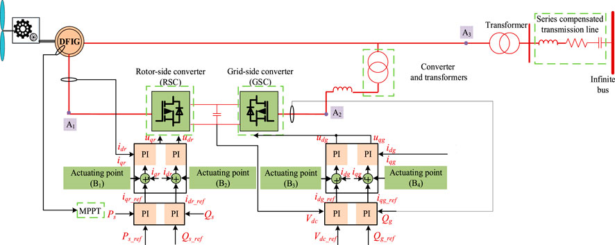
FIGURE 2. DFIG system and the feasible positions of monitoring points and actuating points.

5.1 Mode comprehensive observability metric and mode comprehensive controllability metric calculation

Small-signal model is built in MATLAB/SIMULINK. In the test system, A₁, A₂, A₃ are taken as output signal monitoring points, corresponding to rotor side, grid side and wind farm outlet side respectively. Voltage, current and active power signals are measured as output signals. B₁, B₂, B₃, B₄ are taken as feasible actuating points for input signals, corresponding to the inner loop of active power control (APC) and reactive power control (RPC) of rotor side converter (RSC) and the inner loop of APC and RPC of grid side converter (GSC).

Perform eigenvalue analysis. All eigenvalues are distinct; therefore, we can apply the theory in the first case. The eigenvalues of unstable oscillation are 0.2485 ± 51.8143i, and the corresponding frequency is 8.3 Hz. The oscillation modes corresponding to other eigenvalues are stable. Furthermore, the participation factor analysis is carried out, and the participation coefficients of system components are calculated. It shows in Table 2 that the unstable oscillation mode is strongly related to the components interacting with the subsynchronous control (series capacitor in compensated transmission line). Therefore, the mode can be considered as the dominant mode of subsynchronous oscillation.

TABLE 2

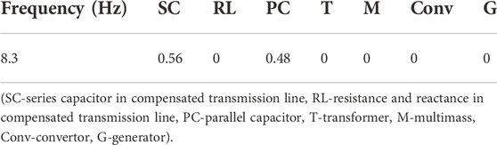
TABLE 2. System component participation coefficients.

5.1.1 Mode comprehensive observability metric calculation and output signal/monitoring point selection

The MCOM of the dominant mode is calculated. It can be seen from Table 3 that the MCOM of dominant mode with current and active power signals in monitoring point A₃ are far greater than that of A₁ and A₂. Therefore, A₃ can better reflect the dominant mode components of subsynchronous oscillation. Moreover, for A3, the MCOM of the current is larger than that of the active power (m_sos (I_q) = 1.596, m_sos (I_d) = 1.279). So, the current of monitoring point A₃ is the most suitable output signal for the system.

TABLE 3

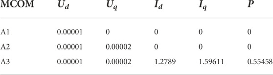
TABLE 3. The MCOM of oscillation mode.

5.1.2 Mode comprehensive controllability metric calculation and subsynchronous damping controller actuating point selection

In order to select the best actuating point for the SSDC, the inner loop of APC and RPC channels of the RSC and GSC is taken as the input signal points, and the MCCM of the dominant mode is calculated. The results are shown in Table 4.

TABLE 4

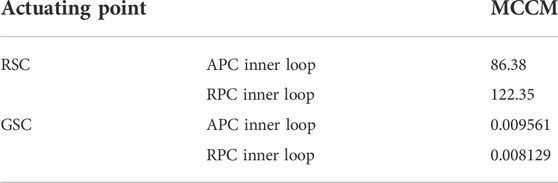
TABLE 4. The MCCM of oscillation mode.

It can be seen from Table 4 that the MCCM of the RSC is greater than that of the GSC, which shows that for the dominant mode, the relative control effect of the SSDC on the RSC is stronger than that of the GSC, i.e., the influence on other oscillation modes is small. Furthermore, actuating point in the inner loop of the RPC has the largest MCCM, so we choose to install SSDC in the inner loop of RPC in RSC.

5.1.3 Modal analysis comparison with and without subsynchronous damping controller

In order to analyze the effectiveness of the result above, the current signal at the outlet of the DFIG is selected as the output signal, and SSDC is installed on the inner loop of the APC and the inner loop of the RPC of the RSC respectively. The system eigenvalues after installing the SSDC are shown in Table 5.

TABLE 5

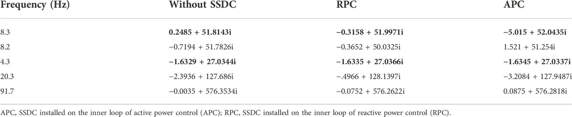
TABLE 5. Eigenvalues of system with SSDC inserted at different points.

It can be seen from Table 5 that compared with the dominant mode damping of subsynchronous oscillation without SSDC, two kinds of SSDC can effectively improve the damping of subsynchronous oscillation. However, when the APC loop is selected as the actuating point, the controller will have a greater control effect on the damping of another oscillation mode (4.8 Hz), and even lead to the negative damping of the mode. The reason is that the frequency of the oscillation mode is 8.2Hz, which is very close to that of the dominant mode. i.e., the control signal in APC loop has a strong influence on the oscillation modes except the dominant mode, which is consistent with the analysis of the MCCM.

In order to better explain the influence of installing additional controllers at different positions on different modes of the system, the variation of damping ratio of different oscillation modes before and after the installation of SSDC is compared, and the results are shown in Figure 3.

FIGURE 3

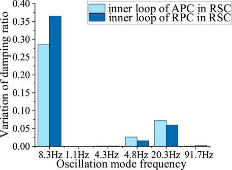
FIGURE 3. Damping ratios of various modes with SSDC at different points.

In the Figure 3, the light color and the dark color respectively show the influence on the system eigenvalues with SSDC installed on the inner loop of the APC and RPC of RSC. It can be seen that compared with the SSDC installed in the APC, the one installed in the RPC has a greater impact on dominant mode, and has less impact on other oscillation modes.

5.1.4 Calculation results of other methods

5.1.4.1 Results of participation factor

The components related to the oscillation mode are determined by the calculation of the participation factor, as shown in Table 2. However, since the state variables are not necessarily measurable, the reflection of the measured variables on the mode cannot be reflected by the participation factor.

5.1.4.2 Results of residue method

Calculate the residue of dominant mode according to Eq. 34. Since residues are often complex numbers, the magnitude of each pair of output signals and input signal/actuating point are shown as Table 6. The output signals (voltage, current and active power) are taken at point A₃. From Table 6, the best output signal and input signal actuating point are current and inner loop of RPC in RSC.

TABLE 6

TABLE 6. The residue of oscillation mode.

5.1.4.3 Results of geometric measures

Calculate geometric measures of dominant mode. From Table 7, the best output signal is current, while from Table 8, the best input signal actuating point is inner loop of RPC in RSC.

TABLE 7

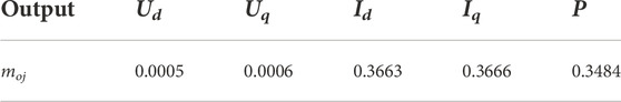
TABLE 7. The m_oj of oscillation mode.

TABLE 8

TABLE 8. The m_cl of oscillation mode.

To summarize, the results of residue, participation factor do not consider the degree of observability and controllability independently, so they are not suitable for the situation where only observability needs to be measured. Besides, the results of residue and geometric measures show the same results as the metrics we proposed. However, as we consider the relative controllability of all the oscillation modes in MCCM, there is a greater difference between results of actuating point in RPC and APC (residue 22%, controllability geometric measure 25%, MCCM 42%). And from Table 5, we can find that the choice of RPC can avoid the damping ratio of 4.3 Hz being positive. Therefore, the results of MCCM are more reliable. Besides, the method of metrics can consider the coupled modes with same oscillation frequency together in system with repeated eigenvalues, which shows less limitation in application scene.

5.2 Application effect analysis with time domain simulation

In order to further confirm the effectiveness of the method above. With same test system shown in Figure 2, the time domain simulation model is established on PSCAD/EMTDC platform. After the system runs stably for 10s, the series compensation capacitor is put in, which causes subsynchronous oscillation with frequency of 8.3 Hz. All the quantities are shown in pu.

5.2.1 Validation of observability metric

Similarly, A₁, A₂ and A₃ are used as output signal monitoring points to compare the performance of voltage, current and active power signals on the dominant mode components. The oscillation waveform is shown in Figure 4.

FIGURE 4

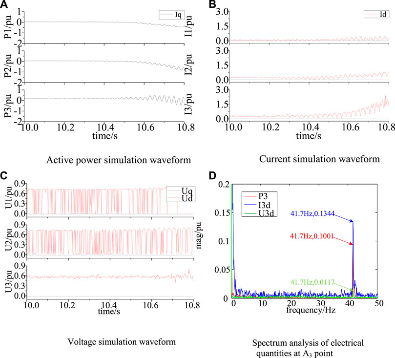
FIGURE 4. Simulations of each monitoring point and spectrum analysis of A₃. (A) Active power simulation waveform (B) Current simulation waveform (C) Voltage simulation waveform (D) Spectrum analysis of electrical quantities at A3 point.

It can be seen from Figures 4A–C that at 10.8s, the oscillation amplitude of power in A₃ is about 0.3, which is greater than A₂ (0.15) and A₁ (0.05); the oscillation amplitude of current in A₃ point is about 0.425, which is greater than A₂ (0.18) and A₁ (0.17), while the change of voltage is not obvious.

In order to intuitively compare the performance of three electrical quantities in A₃, the frequency spectrum of current, voltage and power waveform of monitoring point A₃ is analyzed. In order to improve the resolution of spectrum analysis, take the signals of P₃, I_3d, and U_3d at 10–12s for analysis. The result is shown in Figure 4D. Due to the property of Park transformation, the oscillation frequency is (50-f) Hz, i.e., 41.7 Hz. The oscillation amplitude of the current is 0.1344, and for active power, 0.1001, for voltage, only 0.01. In conclusion, the current in A₃ can better display the dominant mode components of the subsynchronous oscillation, which is consistent with the analysis results of the MCOM.

5.2.2 Validation of controllability metric

Then, the validity of the MCCM is verified. In 12s, the control signals obtained from I₃ through SSDC are input into the inner loop of APC and the inner loop of RPC in RSC respectively (B₁ and B₂). The time-domain simulation results show that the synchronous oscillation can be suppressed under the two control methods. The simulation waveform of suppression with the actuating point in RPC and APC is as Figure 5.

FIGURE 5

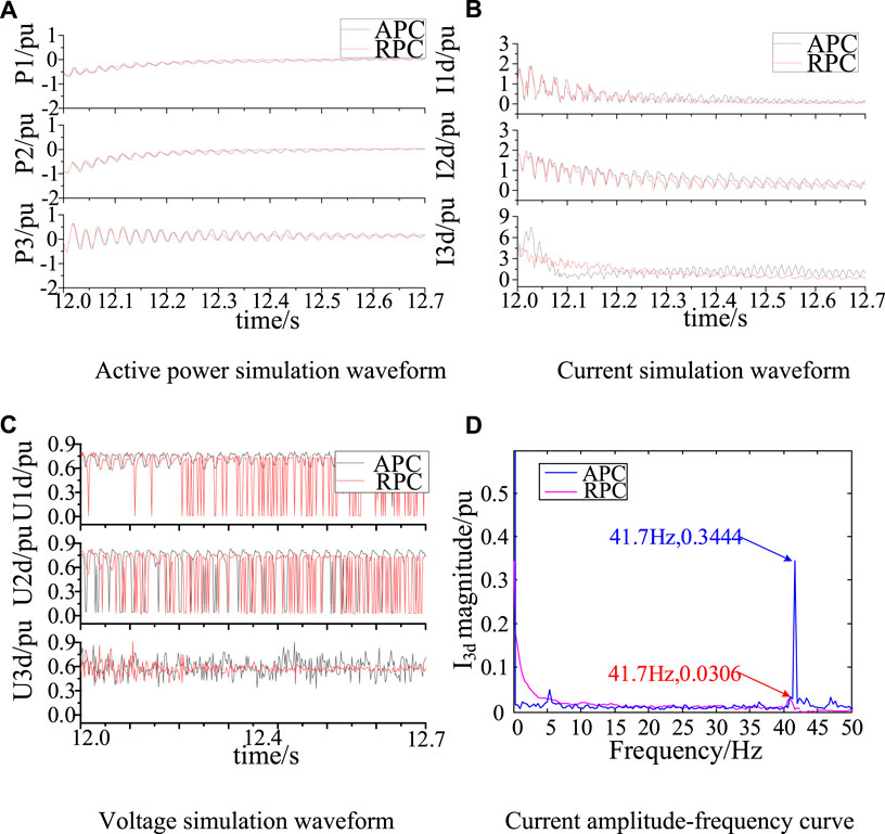
FIGURE 5. Simulations at different monitor points with control in APC and RPC. (A) Active power simulation waveform (B) Current simulation waveform (C)Voltage simulation waveform (D) Current amplitude-frequency curve.

During the simulation time (12s–12.7s), It can be seen that: 1) at 12s, both kinds of SSDC have same oscillation amplitudes. At 12.7s, both of them can suppress the oscillation. 2) From Figure 5, for all the electrical quantities, actuating point in RPC loop has better control effect. Taking the result of P₃ as an example, oscillation amplitude of P₃ is decreased from about 0.5537 to 0.03 with control in RPC, which is less than half of the amplitude with control point in APC (from 0.5537 to 0.07). That is to say, when the actuating point is in RPC loop, the time for each electrical quantity to reach normal is shorter, and the suppression effect is more obvious, which is consistent with the analysis result of MCCM.

To summarize, applying the metrics, it is suggested that in the test power system, the current at the outlet of the wind farm is taken as the output signal, and the SSDC is installed in the inner loop of the RPC channel in RSC. From small-signal model and time-domain model we justify the result, which proves the effectiveness of MCOM and MCCM in the application on the oscillation suppression.

6 Conclusion

In this paper, the definitions of controllability metric and observability metric of oscillation modes are proposed. Based on these concepts, a theoretical system suitable for power systems with distinct or repeated eigenvalues is established. The main conclusions are as follows:

1) Modal observability metric represents the reflection degree of monitoring point measurement on an oscillation mode. Controllability metric characterizes the performance of actuating point control input on an oscillation mode. Compared with the traditional modal analysis methods (residue measure, participation factor measure and geometric measure), CM and OM can reflect the characteristics of oscillation mode, and can be applied to system with or without repeated eigenvalues.

2) The simulation results show that the concepts of MCOM and MCCM are effective and generally applicable to multi-type oscillations of traditional power grid and wind power integrated power grid. By analyzing the results of different methods, it can be found that MCOM and MCCM can measure the degree of observability and controllability independently. And the large value of MCCM means not only strong influence on the dominant mode but also less influence on other oscillation modes, thus it is more reliable.

3) For systems with same repeated eigenvalues, the same eigenvalues cannot be fully decoupled. The MCOM and MCCM are proposed based on the Jordan canonical form of the system state space equation coefficient matrix. They can get rid of the repeated calculation of the same eigenvalues in the process of signal monitoring point and control signal selections by clustering the same eigenvalues into one modal and calculating once. This metric calculation process is simple and has clearer physical meaning.

Data availability statement

The raw data supporting the conclusions of this article will be made available by the authors, without undue reservation.

Author contributions

CZ designed the structure of the study and wrote the manuscript. XW contributed to the conception and idea of the study. ZL and SL built the simulation models. CZ and ZL performed the analysis. XW contributed to manuscript revision, proofreading, and approved the submitted version.

Funding

The Project Supported by National Natural Science Foundation of China (NSFC 51677114, 52077137).

Conflict of interest

The authors declare that the research was conducted in the absence of any commercial or financial relationships that could be construed as a potential conflict of interest.

Publisher’s note

All claims expressed in this article are solely those of the authors and do not necessarily represent those of their affiliated organizations, or those of the publisher, the editors and the reviewers. Any product that may be evaluated in this article, or claim that may be made by its manufacturer, is not guaranteed or endorsed by the publisher.

References

Angulo, M. T., Aparicio, A., and Moog, C. H. (2020). Structural accessibility and structural observability of nonlinear networked systems. IEEE Trans. Netw. Sci. Eng. 7, 1656–1666. doi:10.1109/TNSE.2019.2946535

CrossRef Full Text | Google Scholar

Dobson, I., Zhang, J., Greene, S., Engdahl, H., and Sauer, P. W. (2001). Is strong modal resonance a precursor to power system oscillations? IEEE Trans. Circuits Syst. I. 48, 340–349. doi:10.1109/81.915389

CrossRef Full Text | Google Scholar

Domínguez-García, J. C., Ugalde-Loo, E., Bianchi, F., and Gomis-Bellmunt, O. (2014). Input–output signal selection for damping of power system oscillations using wind power plants. Int. J. Electr. Power & Energy Syst. 58, 75–84. doi:10.1016/j.ijepes.2014.01.001

CrossRef Full Text | Google Scholar

Du, W., Fu, Q., and Wang, H. (2018). Method of open-loop modal analysis for examining the subsynchronous interactions introduced by VSC control in an MTDC/AC system. IEEE Trans. Power Deliv. 33, 840–850. doi:10.1109/TPWRD.2017.2774811

CrossRef Full Text | Google Scholar

Gallardo, C., Herrera, M., Ocaña, M., Guanochanga, E., Camacho, O., and Cuichán, M. (2017). “Optimal location of sliding mode control and power system stabilizers in order to damp electromechanical oscillations using the residue,” in 2017 IEEE PES Innovative Smart Grid Technologies Conference - Latin America (ISGT Latin America), Quito, Ecuador, 20-22 September 2017, 1–6. doi:10.1109/ISGT-LA.2017.8126711

CrossRef Full Text | Google Scholar

Hamdan, H. M. A., and Hamdan, A. M. A. (1987). On the coupling measures between modes and state variables and subsynchronous resonance. Electr. Power Syst. Res. 13, 165–171. doi:10.1016/0378-7796(87)90001-0

CrossRef Full Text | Google Scholar

He, J., Wu, X., Xu, Y., and Guerrero, J. M. (2019). Small-signal stability analysis and optimal parameters design of microgrid clusters. IEEE Access 7, 36896–36909. doi:10.1109/ACCESS.2019.2900728

CrossRef Full Text | Google Scholar

Heniche, A., and Kamwa, I. (2002). Control loops selection to damp inter-area oscillations of electrical networks, Chicago, IL, USA: IEEE Power Engineering Society Summer Meeting, 240. doi:10.1109/PESS.2002.1043224

CrossRef Full Text | Google Scholar

Huang, B., Sun, H., Liu, Y., Wang, L., and Chen, Y. (2019). Study on subsynchronous oscillation in D-PMSGs-based wind farm integrated to power system. IET Renew. Power Gener. 13, 16–26. doi:10.1049/iet-rpg.2018.5051

CrossRef Full Text | Google Scholar

Lei, J., Shi, H., Jiang, P., Tang, Y., and Feng, S. (2019). An accurate forced oscillation location and participation assessment method for DFIG wind turbine. IEEE Access 7, 130505–130514. doi:10.1109/ACCESS.2019.2939871

CrossRef Full Text | Google Scholar

Li, Y., Fan, L., and Miao, Z. (2020). Wind in weak grids: Low-frequency oscillations, subsynchronous oscillations, and torsional interactions. IEEE Trans. Power Syst. 35, 109–118. doi:10.1109/TPWRS.2019.2924412

CrossRef Full Text | Google Scholar

Liu, H., Xie, X., Li, Y., Liu, H., and Hu, Y. (2017). Mitigation of SSR by embedding subsynchronous notch filters into DFIG converter controllers. IET Gener. Transm. &amp. Distrib. 11, 2888–2896. doi:10.1049/iet-gtd.2017.0138

CrossRef Full Text | Google Scholar

Oscullo, J. A., and Gallardo, C. F. (2020). Residue method evaluation for the location of PSS with sliding mode control and fuzzy for power electromechanical oscillation damping control. IEEE Lat. Am. Trans. 18, 24–31. doi:10.1109/TLA.2020.9049458

CrossRef Full Text | Google Scholar

Ping, J., Shuang, F., and Xi, W. (2014). Robust design method for power oscillation damping controller of STATCOM based on residue and TLS-ESPRIT. Int. Trans. Electr. Energy Syst. 24, 1385–1400. doi:10.1002/etep.1779

CrossRef Full Text | Google Scholar

Pratzel-Wolters, D. (1982). “Jordan canonical forms for linear systems,” in 1982 21st IEEE Conference on Decision and Control, Orlando, FL, USA, 08-10 December 1982, 950–951. doi:10.1109/CDC.1982.268285

CrossRef Full Text | Google Scholar

Song, Y., and Blaabjerg, F. (2017). Overview of DFIG-based wind power system resonances under weak networks. IEEE Trans. Power Electron. 32, 4370–4394. doi:10.1109/TPEL.2016.2601643

CrossRef Full Text | Google Scholar

Wang, C., Wen, C., and Lin, Y. (2017). Adaptive actuator failure compensation for a class of nonlinear systems with unknown control direction. IEEE Trans. Autom. Contr. 62, 385–392. doi:10.1109/TAC.2016.2524202

CrossRef Full Text | Google Scholar

Wang, L., Xie, X., Jiang, Q., and Pota, H. R. (2014). Mitigation of multimodal subsynchronous resonance via controlled injection of supersynchronous and subsynchronous currents. IEEE Trans. Power Syst. 29, 1335–1344. doi:10.1109/TPWRS.2013.2292597

CrossRef Full Text | Google Scholar

Wu, D., Tang, F., Dragicevic, T., Vasquez, J. C., and Guerrero, J. M. (2015). A control architecture to coordinate renewable energy sources and energy storage systems in islanded microgrids. IEEE Trans. Smart Grid 6, 1156–1166. doi:10.1109/TSG.2014.2377018

CrossRef Full Text | Google Scholar

Wu, X., Ning, W., Yin, T., Yang, X., and Tang, Z. (2018). Robust design method for the SSDC of a DFIG based on the practical small-signal stability region considering multiple uncertainties. IEEE Access 6, 16696–16703. doi:10.1109/ACCESS.2018.2802698

CrossRef Full Text | Google Scholar

Xie, X., Zhang, X., Liu, H., Liu, H., Li, Y., and Zhang, C. (2017). Characteristic analysis of subsynchronous resonance in practical wind farms connected to series-compensated transmissions. IEEE Trans. Energy Convers. 32, 1117–1126. doi:10.1109/TEC.2017.2676024

CrossRef Full Text | Google Scholar

Zhou, Q., Ding, Y., Mai, K., Bian, X., and Zhou, B. (2019). Mitigation of subsynchronous oscillation in a VSC-HVDC connected offshore wind farm integrated to grid. Int. J. Electr. Power & Energy Syst. 09, 29–37. doi:10.1016/j.ijepes.2019.01.031

CrossRef Full Text | Google Scholar