 Chunyang Gao1
 Xiangyang Yu
- 1College of Water Conservancy and Hydropower Engineering, Xi’an University of Technology, Xi’an, China
- 2PowerChina Northwest Engineering Co., Xi’an, China
The advancement and capacity allocation of variable-speed hydropower units (VSHUs) for suppressing wind power fluctuations are studied. First, a wind–hydropower generation system model, comprising the doubly fed VSHU (DFVSHU) and full-size power VSHU (FSVSHU) is established. Then, three typical operating conditions, namely the wind speed step-up, wind speed sudden drop, and wind gust, are selected to quantify the advantages of the VSHU in suppressing wind power fluctuations using the power range, power standard deviation, and power fluctuation time. Finally, a VSHU capacity allocation scheme in which some FSHUs are transformed into VSHUs for the same total capacity of hydropower units is proposed. A VSHU capacity allocation formula based on this scheme is also proposed. Simulations and comparisons reveal that the VSHU can effectively suppress wind power fluctuations over short time scales, and its effectiveness is 90% higher than that of the FSHU. In addition, the simulation based on the measured wind speed data verifies the effectiveness of the capacity allocation formula. This study provides a new method for suppressing wind power fluctuations over short time scales and provides theoretical guidance for the application of VSHUs through capacity allocation.
1 Introduction
Carbon peaking and neutrality in the power industry are essential for guaranteeing the “double carbon target.” Clean energy, especially wind power generation, must be incorporated into the power grid on a large scale to achieve this target (Han et al., 2021). According to the Global Wind Energy Council (GWEC), the global wind power installed capacity increased by 93.6 GW in 2021, with China experiencing an increase of 47.6 GW (Global Wind Energy Council, 2022). By the end of 2021, the installed capacity of wind power in China reached 3300 GW, accounting for 13.87% of the total installed capacity in the nation (Yao, 2022). However, the fluctuation, randomness, and intermittence of wind power create power fluctuations that considerably affect the power grid’s stability and quality (Barra et al., 2021).
According to the different time scales, wind power fluctuations can be divided into short time scales (within 1 min), medium time scales (several minutes to tens of minutes), and long time scales (above 1 h), and the measures to suppress the wind power fluctuation are different (Wang and Jiang, 2014). The measures used to suppress wind power fluctuation over short time scales must have sufficient response speeds and power densities, whereas those used to suppress wind power fluctuation over medium time scales must have sufficient energy densities. Those for suppressing wind power fluctuation over long time scales must have sufficient energy storage capacities. The fixed speed hydropower unit (FSHU) has a large energy storage capacity, rapid starts and stops, and convenient output regulation, which allow for the effective suppression of wind power fluctuation over long time scales. However, owing to the slow power response speed and the anti-regulation characteristics of the FSHU, it cannot effectively suppress wind power fluctuations over short time scales (Wang et al., 2020). Therefore, wind–hydro power generation systems usually require additional measures to suppress wind power fluctuations over short time scales (de Siqueira and Peng, 2021).
Currently, two main measures are used to suppress wind power fluctuations over short time scales (Xu et al., 2017). One is direct power control without auxiliary energy storage, which suppresses the power fluctuations of a unit through its own regulation control, such as rotor kinetic energy storage (Varzaneh et al., 2014), pitch control (Xu et al., 2017), and DC bus voltage control (Uehara et al., 2011). Although these methods can stabilize the power fluctuations of the unit over short time scales, they have limited regulating capacity, reduce the wind energy utilization rate, and may damage the wind turbine (Howlader et al., 2013). The second measure used is the auxiliary stabilization method of the external energy storage device, which suppresses the unit’s power fluctuations through fast energy storage device, such as compressed air energy storage devices (Yang et al., 2021), batteries (de Siqueira and Peng, 2021), supercapacitors (Muyeen et al., 2008), and flywheel energy storage devices (Jerbi et al., 2009). These measures have a significant stabilization effect and are very widely used. They can be used together with the WHPGS to form a wind–hydro–storage power generation system (WHSPGS). However, they have disadvantages such as increased cost, a short service life, and a limited configuration capacity.
The variable-speed hydropower unit (VSHU) employing power electronic technology has a fast response speed (Gao et al., 2021a) and does not have anti-regulation characteristics, making it possible to suppress the wind power fluctuations over a short time scale (Iliev et al., 2019). For example, the VSHU of the Ohkawachi Pumped Storage Plant in Japan can change the power output by at least 32 MW within 0.2 s. However, the present research on VSHUs mainly focuses on modelling and control strategy design (Gao et al., 2021b; Fu et al., 2022), and few studies have conducted quantitative analysis on the advancement of VSHUs in suppressing wind power fluctuations over short time scales. Therefore, three typical wind speed conditions are selected in this study to determine and quantify the advancement of VSHU in suppressing wind power fluctuations by using the power range, standard deviation, and fluctuation time.
Capacity allocation is important for suppressing wind turbine power fluctuations (Wang and Jiang, 2014). For the WHSPGS composed of FSHUs, the capacity of the hydropower units and energy storage capacity of the system must be determined (Huang et al., 2011). The capacity allocation of FSHUs is a long time scale, which mainly considers the shortage of power and electricity. The goal is to address is how to reasonably use the long-term regulation and storage capacity of the FSHU’s reservoir (Chang et al., 2015). The capacity allocation of the energy storage system is a short time scale, which focuses on power quality, and its goal is to use rapid power regulation to smooth the short time scale wind power fluctuations. The VSHU can account for wind power fluctuations over long- and short-time scales. The capacity allocation is different from that of FSHU or energy storage system, and must be investigated. Presently, there are few studies on the capacity allocation of VSHUs, which is an important theoretical guidance for unit application. Therefore, after analyzing the advancement of VSHUs, we study their capacity allocation strategy and verify it with actual wind speed data.
In summary, this study investigates the advancement and capacity allocation of the VSHU in suppressing wind power fluctuations. The main contributions of this study are as follows: 1) The advancement of the VSHU is quantified using simulations and calculations; 2) a new method that suppresses wind power fluctuations over short time scales is proposed; and 3) a capacity allocation strategy that can provide theoretical guidance for the application of VSHU is also proposed. The results in this study can provide schemes for some scenarios, such as using variable-speed tubular hydropower units to suppress the power fluctuations of offshore wind power on isolated islands.
2 WHPGS model
2.1 WPGU model
The WPGU model comprises a wind turbine, a permanent magnet synchronous generator (PMSG), pitch angle control, a converter, machine-side control (MSC), and grid-side control (GSC). Its structure is shown in Figure 1.
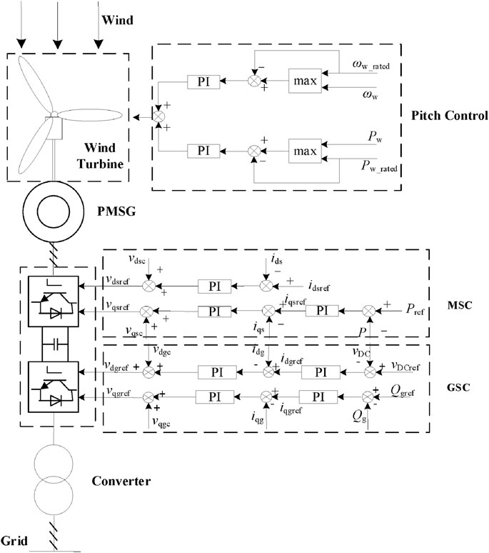
FIGURE 1. Structure of the WPGU.
2.1.1 Wind turbine model
The mechanical torque obtained by the wind turbine is
where PW is the output power of the WPGU, ρ is the air density, R is the wind turbine impeller radius, CP is the wind turbine power factor, β is the pitch angle, ωw is the wind turbine speed, λ is the tip wind speed ratio, v is the wind speed, and Tm_w is the mechanical torque of the wind turbine.
The expression for CP can be approximated as (Chen and Wu, 2011)
where i is the time node.
2.1.2 PMSG model
The PMSG model adopts the dynamic model under dq synchronous rotating coordinates, which mainly includes the stator voltage, stator flux, electromagnetic torque, and motion equations.
(1) Stator voltage equation:
where vds and vqs are the d and q axis components of the stator voltage, respectively; φds and φqs are the d and q axis components of the rotor flux chain, respectively; ids and iqs are the d and q axis components of the stator current, respectively; ω1 is the synchronous angular velocity; and Rs is the generator stator resistance.
(2) Stator flux equation:
where φf is the permanent magnet flux chain, and Lds and Lqs represent the d and q axis components of the stator winding inductance, respectively.
(3) Electromagnetic torque equation:
where Te represents the electromagnetic torque of the generator, and np represents the number of poles.
(4) Motion equation:
where H represents the inertia constant of the generator.
2.1.3 Pitch angle control strategy
The pitch angle control strategy includes a speed control loop and a power control loop, as shown in Figure 1. For the speed control loop, if the rotational speed ωw is greater than the rated rotational speed ωw_rated, the pitch angle is increased through the PI controller to reduce the wind energy utilization rate of the unit. For the power control loop, if the power output of the WPGU P is greater than the rated power output of the WPGU Pw_rated, the pitch angle is increased through the PI controller. When the wind turbine operates in the maximum power point tracking (MPPT) mode, the pitch angle is always kept at 0°.
2.1.4 Converter model
The converter adopts a dual pulse width modulation (PWM) model, and its structure is shown in Figure 2. The PWM near the generator side is called the MSC, and the PWM near the power grid is called the GSC. The machine side converter model is the generator model, and the grid side converter and DC bus model are given by
where vDC is the bus voltage; vdg and vqg are the d and q axis components of the GSC voltage, respectively; idg and iqg are the d and q axis components of the GSC current, respectively; C is the capacitance; vd and vq are the d and q axis components of the grid voltage, respectively; L is the AC side filter inductance; and R is the parasitic resistance in the inductance.
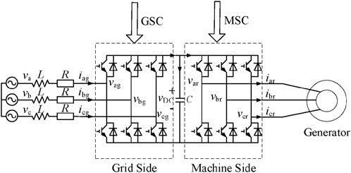
FIGURE 2. Structure of the converter.
2.1.5 Machine-side control (MSC)
MSC adopts a vector control strategy (rotor magnetic field orientation) with a stator reference value of zero (idsref = 0). Its strategy control block diagram is shown in Figure 1, where Pref is the reference power; idsref and iqsref are the current reference values of the stator d and q axes, respectively; vdsref and vqsref are the d and q axis reference values of the stator voltage, respectively; and vdsc and vqsc represent the voltage compensation terms at the generator side, respectively:
2.1.6 Grid-side control (GSC)
GSC adopts double closed-loop control based on the voltage direction. Its structure is shown in Figure 1, where vDCref is the bus voltage reference value; Qgref is the reactive power reference value of the GSC; idgref and iqgref are the d and q axis reference values of the GSC current, respectively; vdgref and vqgref are the d and q axis reference values of the GSC voltage, respectively, which are expressed as
2.2 DFVSHU model
The DFVSHU model primarily includes a doubly fed induction generator (DFIG), hydraulic turbine, water diversion system, double PWM converter, DFIG control system, and hydraulic turbine control system, as shown in Figure 3. The converter model can refer to Eq. 7. The GSC can refer to Eq. 9. The mathematical descriptions of other models are as follows.
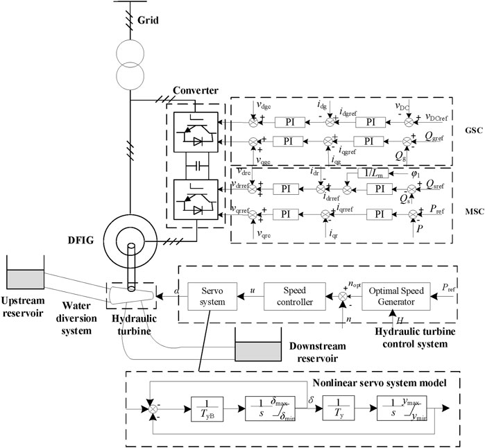
FIGURE 3. Structure of the DFVSHU.
2.2.1 Hydraulic turbine model
The hydraulic turbine model is characterized by the torque and flow characteristics under steady-state conditions, which are given as
where α is the opening of the turbine, n is the turbine speed, H is the head, and Mt is the torque of the turbine.
2.2.2 Water diversion system model
The water diversion system adopts the approximate elastic water hammer model:
where Tw is the inertia time constant of the water flow, Tr is the reflection time constant of the water hammer pressure wave, and f is the head loss coefficient.
2.2.3 Hydraulic turbine control system model
The hydraulic turbine control block diagram of the DFVSHU is shown in Figure 3, in which nopt is the optimal speed of the turbine, and u is the output of the speed controller. Details on the optimal speed generator have been provided by Gao et al. (2021b).
The speed controller adopts a proportional–integral–derivative (PID) controller, and its transfer function can be expressed as
where KP, KI, and KD represent proportional, integral, and differential control parameters, respectively.
The servo system adopts a nonlinear servo system model considering the speed limit, position limit, governor position saturation limit, and suppression of the servomotor. The model block diagram is shown in Figure 3, where δ is the stroke of the pressure distribution valve; TyB is the response time constant of the auxiliary servomotor; Ty is the response time constant of the servomotor; δmax and δmin are the upper and lower limits of the pressure distribution valve stroke, respectively; and ymax and ymin are the upper and lower limits of the relay stroke, respectively.
2.2.4 DFIG model
The DFIG model adopts the dynamic equations of the synchronous rotating coordinate system: the voltage, flux linkage, torque, and motion equations.
(1) Voltage equations:
The stator voltage equation is
The rotor voltage equation is
where vdr and vqr are the d and q axis components of the rotor voltage, respectively; φdr and φqr are the d and q axis components of the rotor flux, respectively; idr and iqr are the d and q components of the rotor current, respectively; Rr is the rotor resistance of the generator; and ωr is the rotor angular velocity.
(2) Flux linkage equations:
The stator flux linkages equation is
The rotor flux linkages equation is
where Lm is the mutual inductance between the stator and rotor windings, Ls is the self-inductance of the stator windings, and Lr represents the self-inductance of the rotor windings.
(3) Torque equation:
(4) Motion equation:
where Tm represents the mechanical moment of the hydraulic turbine, which is consistent with Mt in Eq. 10.
2.2.5 Machine-side control (MSC)
MSC adopts double closed-loop control based on the stator flux direction, as shown in Figure 3, where φ1 is the stator flux linkage based on stator flux direction; idrref and iqrref are the d and q axis components of the rotor current reference, respectively; and vdrref and vqrref are the d and q axis components of the rotor voltage reference, respectively; vdrc and vqrc are the voltage compensation terms at the rotor side, respectively, which are expressed as
2.3 FSVSHU model
The FSVSHU model mainly consists of the turbine system, water diversion system, turbine control system, permanent magnet generator, converter, machine-side vector control, and grid-side vector control. Its structure is shown in Figure 4.
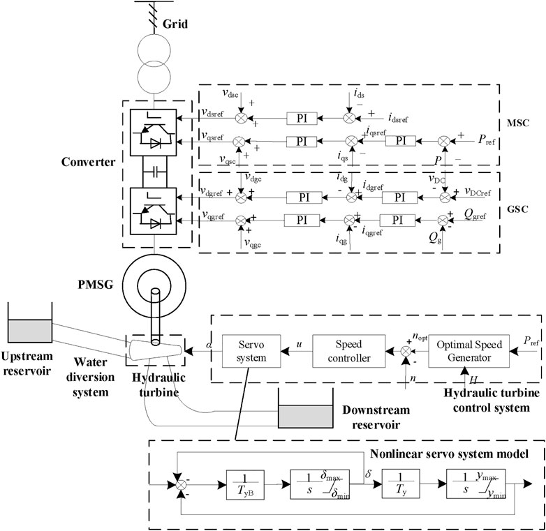
FIGURE 4. Structure of the FSVSHU.
The models of the hydraulic turbine, water diversion system, and hydraulic turbine control system are described by Eq. 10, Eq. 11 and Eq. 12, respectively. The PMSG, GSC, and MSC models are described by Eq. 3, Eq. 7 and Eq. 9, respectively. The structured of the MSC and hydraulic turbine control system are illustrated in Figure 4.
2.4 WHPGS model
The structure of the WHPGS is shown in Figure 5.
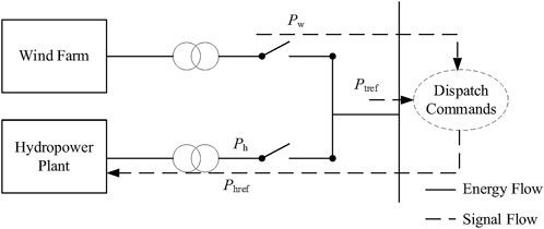
FIGURE 5. Structure of the WHPGS.
In actual operation, the power reference value of the hydropower unit Phref can be calculated from the current dispatching command Ptref and the power Pw currently issued by the wind farm (Phref = Ptref -Pw). A change in wind speed causes changes in Pw and Phref, and the hydropower unit adjusts the power output Ph of the unit according to Phref to stabilize the wind power.
3 Analysis of the VSHU advantages in suppressing wind power fluctuations over short time scales
Before conducting the analysis, the capacity of the hydropower unit and the WPGU should be determined. In general, to eliminate the influence of wind power randomness on the power grid, the regulating capacity of the hydropower unit in the WHPGS must be equivalent to that of the wind power unit (Huang et al., 2011). Therefore, the capacities of the WHPGS and hydropower unit are set at a 1:1 ratio in this section. The advantages of the VSHU are illustrated by choosing an actual 100 MW wind farm as the simulation object. The wind farm consists of a 40 × 2.5 MW WPGU. The simulation assumes that the real-time state of the 40 wind turbines is exactly the same.
3.1 Simulation condition settings
The power fluctuations of the wind power over a short time scale can be realized by simulating the power fluctuation of the wind turbines within 1 min. In actual operation, wind turbines mainly operate in the MPPT mode, and the power fluctuations generally correspond to fluctuations in the MPPT mode. Therefore, this paper selects three typical working conditions in the MPPT mode for simulation: the wind speed step-up, wind speed sudden drop, and wind gust.
To accurately describe the wind fluctuations over short time scales, the wind model adopts a four-component wind model. The wind in this model is a combination of basic, gradient, gust and random wind. Basic wind and gradual wind represent the linear component of the wind, while gust and random wind represent the linear component of the wind. And it can be expressed as
where v1 is basic wind, v2 is gust wind, v3 is gradual wind, and v4 is random wind.
The basic wind v1 always exists during normal operation of the wind turbine, and reflects the average wind speed of the wind farm, which is generally regarded as a constant and can be obtained through the Weibull distribution of wind speed.
The gust v2 refers to the wind that suddenly appears and disappears. It reflects the sudden change in wind speed characteristics and can be simulated using the following trigonometric function:
where ts2 is the gust start time, te2 is the gust end time, and v2a is the gust amplitude.
The gradual wind refers to the wind speed rising or falling slowly. It reflects the gradual characteristics of wind speed and can be simulated using the following slope function:
where ts3 is the gradual wind start time, te3 is the gradual wind end time, and v3a is the gradual wind amplitude.
The random wind is a component of wind speed caused by wind irregularity. It reflects the wind speed’s random variability and can be simulated by adding white noise:
where v4max is the random wind amplitude, rand (−1,1) represents a random number between −1 and 1; φi represents a random number between 0 and 2π, and ωi is the frequency of each frequency band.
The wind speed data used in the simulation are obtained from historical data. The basic wind amplitude is 6.72 m/s, the maximum gust amplitude is 4 m/s, the maximum gradual wind amplitude is 4 m/s, and the maximum random wind amplitude is 1 m/s. Therefore, the three typical working conditions can be simulated according to the above description.
3.2 Wind speed step-up
Wind speed step-up is an actual phenomenon characterized by stepwise increases in wind speed that can be simulated by the superposition of basic, random, and two gradual upper winds. In the simulation, the duration of the gradual wind on both occasions is 2 s, the gradual wind speed is 1.5 m/s, the basic wind speed is 6.72 m/s, and a small random wind is applied.
The simulation duration is set to 60 s, and the results are shown in Figure 6A.
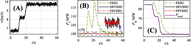
FIGURE 6. Simulation results for the wind speed step-up condition: (A) Simulation results for the wind speed; (B) power changes of different WHPGS types; (C) power outputs of different VSHU types.
The value of Ptref is set to 100 MW for the simulation. Figure 6B shows the power changes for different WHPGS types. The power outputs for different VSHU types are shown in Figure 6C.
According to Figure 6B, under the wind speed step-up condition, the WHPGS composed of FSHU have two large power fluctuations, with the second fluctuation being greater than the first. The first fluctuation, which occurs at 13.41 s (3.41 s after the first fluctuation of wind speed), has a maximum value of 113.11 MW, and the second fluctuation, which occurs at 21.73 s (3.73 s after the second fluctuation of wind speed), has a maximum value of is 118.09 MW. The WHPGSs composed of VSHU have similar effects and two power fluctuations. The first and second fluctuations occur at approximately 12.50 s and 21.50 s, respectively, and the power fluctuations are within ±1% of the capacity of the WPGU. According to Figure 6C, under the wind speed step-up condition, the FSHU cannot accurately follow the Phref before 44.40 s (24.40 s after the end of wind speed fluctuation), and there are two anti-regulation characteristics. The first and second anti-regulation characteristics occur at 12.68 and 20.51 s, respectively, and their maximum values are 87.25 and 75.70 MW, respectively. The two types of VSHU can accurately follow the Phref.
To quantify the advantages of the VSHU, the power range D, the power standard deviation σ, and the power fluctuation time within 1 min are calculated, as shown in Table 1. The power fluctuation time is the time when the power fluctuations exceed ±1% of the capacity of the WPGU.
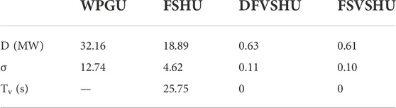
TABLE 1. Quantitative comparison of different WHPGS types (wind speed step-up).
According to Table 1, under the wind speed step-up condition, the power range of the WHPGS composed of FSHU is 18.89 MW, which is 13.27 MW lower than that of the WPGU. The power standard deviation is 4.62, which is 8.12 less than that of the WPGU. These results indicate that the FSHU plays a small role in suppressing wind power fluctuations under the wind speed step-up condition. When the DFVSHU is adopted, the power range of WHPGS is 0.63 MW (96.67% lower than that of the FSHU), and the power standard deviation is 0.11 (97.62% lower than that of the FSHU). The power fluctuation time changes from 25.75 to 0 s. When the FSVSHU is adopted, the power range of the WHPGS is 0.61 MW (96.77% lower than that of the FSHU), and the power standard deviation is 0.10 (97.83% lower than that of the FSHU). The power fluctuation time changes from 25.75 to 0 s.
3.3 Wind speed sudden drop
Wind speed sudden drop is an actual wind loss phenomenon that can be simulated by the superposition of basic, random, and gradual winds. In this case, the final wind speed of the wind speed step-up working condition is the initial wind speed of the wind speed sudden drop condition (9.72 m/s). The amplitude of the gradual wind is 4 m/s, and its duration is 4 s (10–14 s). A small amplitude random wind is applied. The simulation duration is set to 60 s, and the results are shown in Figure 7A.
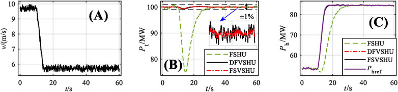
FIGURE 7. Simulation results for the wind speed sudden drop condition: (A) Simulation results for wind speed; (B) power changes of different WHPGS types; (C) power outputs of different VSHU types.
The value of Ptref is set to 100 MW for the simulation. Figure 7B shows the power changes for different WHPGS types. The power outputs for different VSHU types are shown in Figure 7C. The power range D, the power standard deviation σ, and the power fluctuation time within 1 min are shown in Table 2.
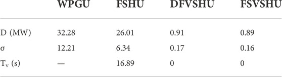
TABLE 2. Quantitative comparison of different WHPGS types (wind speed sudden drop).
According to Figure 7B, when the wind speed suddenly drops, the WHPGS composed of the FSHU exhibits a large power fluctuation. The minimum fluctuation occurs at 14.73 s (4.73 s after the wind speed fluctuation) and has a value of 75.01 MW. The WHPGSs composed of the VSHU also have power fluctuations, with the minimum fluctuation occurring at approximately 14 s, and the power fluctuations are within ±1% of the capacity of the WPGU. According to Figure 7C, under the wind speed sudden drop condition, the FSHU cannot accurately follow the Phref until 33.40 s (19.40 s after the end of wind speed fluctuation), and it exhibits an anti-regulation characteristic. The minimum value of the anti-regulation, which occurs at 12.05 s, is 51.75 MW. The two types of VSHU can accurately follow the Phref.
According to Table 2, under the wind speed sudden drop condition, the power range of the WHPGS composed of the FSHU is 26.01 MW, which is 6.27 MW lower than that of the WPGU. The power standard deviation is 6.34, which is 5.87 less than that of the WPGU. These results indicate that the FSHU plays a small role in suppressing wind power fluctuations when wind speed suddenly drops. When the DFVSHU is adopted, the power range of the WHPGS is 0.91 MW (96.26% lower than that of the FSHU), and the power standard deviation is 0.17 (97.32% lower than that of the FSHU). The power fluctuation time changes from 16.89 to 0 s. When the FSVSHU is used, the power range of the WHPGS is 0.89 MW (96.26% lower than that of the FSHU), and the power standard deviation is 0.16 (97.4% lower than that of the FSHU). The power fluctuation time changes from 16.89 to 0 s.
3.4 Wind gust
A wind gust is an actual phenomenon in which the wind speed increases and recovers in a short time. Under this condition, the basic wind is 6.72 m/s, the gust amplitude is 3.6 m/s, and the duration is 6 s (20–26 s). A small-amplitude random wind is also used. The simulation duration is set to 60 s, and the results are shown in Figure 8A.
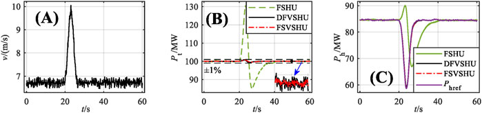
FIGURE 8. Simulation results for the wind gust condition: (A) Simulation results for wind speed; (B) power changes of different WHPGS types; (C) power outputs of different VSHU types.
The Ptref value is set to 100 MW for the simulation. Figure 8B shows the power changes for different WHPGS types. The power outputs for different VSHU types are shown in Figure 8C. The power range D, the power standard deviation σ, and the power fluctuation time within 1 min are shown in Table 3.
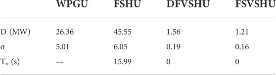
TABLE 3. Quantitative comparison of different WHPGS types (wind speed sudden drop).
According to Figure 8B, under the wind gust condition, the WHPGS composed of FSHU has two large power fluctuations. The first fluctuation occurring at 23.52 s (3.52 s after the wind speed fluctuation) is positive, with the maximum value of 130.64 MW, and the second fluctuation occurring at 27.11 s (7.11 s after the wind speed fluctuation) is negative, with the minimum value of 85.21 MW. The WHPGSs composed of VSHU also has positive and negative power fluctuations occurring at about 23 and 26 s, respectively, and the power fluctuations are within ±1% of the capacity of the WPGU. According to Figure 8C, under the wind gust condition, the FSHU cannot accurately follow the Phref until 40.83 s (14.83 s after the end of wind speed fluctuation), and there is an anti-regulation characteristic. The maximum value of the anti-regulation is 90.05 MW, and it occurs at 23.16 s. The two types of VSHU can accurately follow the Phref.
According to Table 3, under the wind gust condition, the power range of the WHPGS composed of the FSHU is 45.55 MW, which is 19.19 MW more than that of the WPGU. The power standard deviation is 6.05, which is 1.04 more than that of the WPGU. These results indicate that the FSHU aggravates wind power fluctuations under the wind gust condition. When the DFVSHU is adopted, the power range of the WHPGS is 1.56 MW (96.58% lower than that of the FSHU), and the power standard deviation is 0.31 (97.34% lower than that of the FSHU). The power fluctuation time changes from 15.99 to 0 s. When the FSVSHU is adopted, the power range of the WHPGS is 1.21 MW (96.86% lower than that of the FSHU), and the power standard deviation is 0.19 (97.35% lower than that of the FSHU). The power fluctuation time changes from 15.99 to 0 s.
3.5 Summary
In summary, the FSHU cannot suppress wind power fluctuations over short time scales. When the wind speed step-up and suddenly drops, the FSHU plays a small role in suppressing wind power fluctuations and requires a long time to supplement the power shortage of the WHPGS. For conditions with large amplitude and short time fluctuations, such as wind gust conditions, the FSHU can even adversely affect the power stability, resulting in a larger power fluctuation.
Under the three typical working conditions, the two VSHU types demonstrated good power stabilization effects. The output power of the WHPGS was stable at ±1% of the capacity of the WPGU. The power range and the power standard deviation decreased significantly by more than 90%. These results reveal that VSHUs are effective at suppressing the power fluctuations of the WPGU over short time scales.
4 VSHU capacity allocation
4.1 VSHU capacity allocation in the WHPGS
Generally, the primary function of the hydropower unit in the WHPGS is to supplement the power and electricity balance in the system. Without considering the constraints of water balance and upstream and downstream water levels, the regulating capacity of the hydropower unit should be equivalent to that of the WPGU. Power and electricity shortages correspond to WPGU power fluctuations over long time scales. When the FSHU is adopted in the WHPGS to suppress the WPGU power fluctuations over short time scales, the WHPGS requires additional fast energy storage equipment, such as batteries and supercapacitors. When the VSHU is adopted in the WHPGS, the system only needs to be equipped with a particular VSHU instead of fast energy storage devices. Therefore, the economical and feasible approach is to transform some units in the WHPGS into VSHUs under the condition that the total capacity of the hydropower units is equivalent to that of the WPGU.
4.2 Capacity allocation of the VSHU for suppression of wind power fluctuations over short time scales
The capacity allocation of a VSHU used to suppress the wind power fluctuations over short time scales can refer to the method of using batteries and supercapacitors. However, the difference is that the VSHU can only generate power and cannot absorb electric energy. Therefore, the expected power of the VSHU–WPGU system should be equal to the maximum power fluctuation of the WPGU, and the capacity of the VSHU should be the maximum value of the power range of the WPGU. Under the condition that the WHPGS power fluctuation is stable at ±1% of the WPGU capacity, the VSHU capacity (i.e., the maximum power output) can be expressed as
where Phmax is the maximum power output of the VSHU, Dwmax is the maximum value of the power range of the WPGU, and Prw represents the rated power of the WPGU.
4.3 Example simulation
An actual wind speed sample was used in the simulation, as shown in Figure 9A. The corresponding power output of the WPGU is shown in Figure 9B.
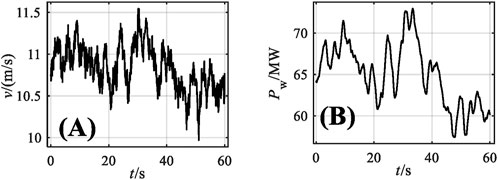
FIGURE 9. An actual wind speed simulation: (A) Historical wind speed data; (B) corresponding power output of the WPGU.
According to Figure 9, the maximum WPGU power fluctuation value is 72.97 MW, the minimum power fluctuation value is 57.89 MW, and the maximum power range value is 15.08 MW. Therefore, the expected power of the wind power hydropower system should be set to 72.97 MW, and the VSHU capacity should be 16.08 MW.
The power of the VSHU–WPGU system equipped with the VSHU is shown in Figure 10. The shaded part in the figure is the VSHU power, the solid line is the power of the VSHU–WPGU system, and the dotted line is the power of the WPGU.
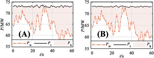
FIGURE 10. Power of the VSHU–WPGU system: (A) DFVSHU; (B) FSVSHU.
According to Figure 10, for the simulation of actual wind speed samples, the power of the DFVSHU-WPGU system fluctuates between 72.31 and 73.65 MW, and the power of the FSVSHU-WPGU system fluctuates between 72.57 and 73.37 MW. The power fluctuation range of the VSHU–WPGU systems are within ±1% of the WPGU capacity, which shows that the capacity allocation strategy proposed in this paper is effective.
Further, a comparison of the DFVSHU and FSVSHU is shown in Figure 11. According to Figure 11, when the DFVSHU is adopted, the power change rate of the system is 0.68%. When the FSVSHU is employed, the power change rate of the system is 0.40%. These results reveal that the FSVSHU is more effective at regulating power than the DFVSHU.
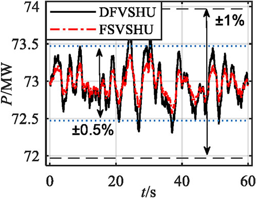
FIGURE 11. Comparison of the DFVSHU and FSVSHU.
5 Conclusion
The advancement and capacity allocation of the VSHU in suppressing wind power fluctuations are analyzed in this paper, and the following conclusions are drawn:
(1) The VSHU noticeably suppresses wind power fluctuations over short time scales. Under typical wind speed conditions, the power range, power standard deviation, and power fluctuation time of a WHPGS composed of either of the two VSHU types are 90% lower than those of the FSHU. These results highlight the advancement of VSHUs. Furthermore, they reveal that the VSHU is a novel and effective method which can be used for suppressing wind power fluctuations over short time scales.
(2) When using the VSHU to suppress wind power fluctuations over short time scales, the economical and feasible approach is to transform some FSHUs into VSHUs under the condition that the total capacity of hydropower units is equivalent to that of the WPGU. The expected power of the VSHU–WPGU system should be equal to the maximum power fluctuation of the WPGU, and the capacity of the VSHU should be the maximum power range of the WPGU. This provides a theoretical guidance for the application of VSHUs.
(3) The FSVSHU suppresses the WPGU power fluctuations over short time scales more effectively than the DFVSHU. This provides a reference for the selection of variable speed units in practice.
(4) This paper mainly studies the role of VSHUs in suppressing wind power fluctuations over short time scales; however, their performance over long time scales should also be studied. When conducting long-time scale research, the water balance, upstream and downstream water levels, available water, and other constraints of hydropower stations must be considered. These considerations will be the next research focus of our research group (Jannati et al., 2014; Xie et al., 2021).
Data availability statement
The original contributions presented in the study are included in the article/supplementary materials, further inquiries can be directed to the corresponding authors.
Author contributions
CG and XY: Methodology; CG and ZZ: Software; CG and HN: Validation; CM and LW: Data curation; CG and ZZ: Writing—original draft preparation; LW and HN: Writing—review and editing; CG: Visualization; QC: Supervision; and XY and HN: Project administration.
Funding
National Key R&D Program of China (Grant No. 2018YFB1501900), National Natural Science Foundation of China (Grant No. 52179090), and Natural Science Basic Research Plan in Shaanxi Province of China (Grant No. 2019JQ-742).
Conflict of interest
ZZ was employed by PowerChina Northwest Engineering Co.
The remaining authors declare that the research was conducted in the absence of any commercial or financial relationships that could be construed as a potential conflict of interest.
Publisher’s note
All claims expressed in this article are solely those of the authors and do not necessarily represent those of their affiliated organizations, or those of the publisher, the editors and the reviewers. Any product that may be evaluated in this article, or claim that may be made by its manufacturer, is not guaranteed or endorsed by the publisher.
References
Barra, P. H. A., de Carvalho, W. C., Menezes, T. S., Fernandes, R. A. S., and Coury, D. V. (2021). A review on wind power smoothing using high-power energy storage systems. Renew. Sustain. Energy Rev. 137, 110455. doi:10.1016/j.rser.2020.110455
Chang, J., Wang, Y., Huang, Q., and Sun, X. (2015). Compensation operation mechanism of hydropower plant and windpower plant. J. Hydroelectr. Eng. 33, 68–73+80.
Chen, B., and Wu, Z. (2011). Power smoothing control strategy of doubly-fed induction generator based on constraint factor extent-limit control. Proc. CSEE 31, 130–137. doi:10.13334/j.0258-8013.pcsee.2011.27.018
de Siqueira, L. M. S., and Peng, W. (2021). Control strategy to smooth wind power output using battery energy storage system: A review. J. Energy Storage 35, 102252. doi:10.1016/j.est.2021.102252
Fu, J., Yu, X., Gao, C., Cui, J., and Li, Y. (2022). Nonsingular fast terminal control for the DFIG-based variable-speed hydro-unit. Energy 244, 122672. doi:10.1016/j.energy.2021.122672
Gao, C., Yu, X., Nan, H., Men, C., and Fu, J. (2021a). A fast high-precision model of the doubly-fed pumped storage unit. J. Electr. Eng. Technol. 16, 797–808. doi:10.1007/s42835-020-00641-0
Gao, C., Yu, X., Nan, H., Men, C., Zhao, P., Cai, Q., et al. (2021b). Stability and dynamic analysis of doubly-fed variable speed pump turbine governing system based on Hopf bifurcation theory. Renew. Energy 175, 568–579. doi:10.1016/j.renene.2021.05.015
Global Wind Energy Council (Gwec), (2022). Global wind report 2022 bonn. https://gwec.net/global-wind-report-2022/.
Han, X., Li, T., Zhang, D., and Zhou, X. (2021). New issues and key technologies of new power system planning under double carbon goals. High. Volt. Eng. 47, 3036–3046. doi:10.13336/j.1003-6520.hve.20210809
Howlader, A. M., Urasaki, N., Yona, A., Senjyu, T., and Saber, A. Y. (2013). A review of output power smoothing methods for wind energy conversion systems. Renew. Sustain. Energy Rev. 26, 135–146. doi:10.1016/j.rser.2013.05.028
Huang, C., Ding, J., Tian, G., and Tang, H. (2011). Hydropower operation modes of large-scale wind power grid integration. Autom. Electr. Power Syst. 35, 37–40+111.
Iliev, I., Trivedi, C., and Dahlhaug, O. G. (2019). Variable-speed operation of francis turbines: A review of the perspectives and challenges. Renew. Sustain. Energy Rev. 103, 109–121. doi:10.1016/j.rser.2018.12.033
Jannati, M., Hosseinian, S. H., Vahidi, B., and Li, G. J. (2014). A survey on energy storage resources configurations in order to propose an optimum configuration for smoothing fluctuations of future large wind power plants. Renew. Sustain. Energy Rev. 29, 158–172. doi:10.1016/j.rser.2013.08.086
Jerbi, L., Krichen, L., and Ouali, A. (2009). A fuzzy logic supervisor for active and reactive power control of a variable speed wind energy conversion system associated to a flywheel storage system. Electr. Power Syst. Res. 79, 919–925. doi:10.1016/j.epsr.2008.12.006
Muyeen, S. M., Shishido, S., Ali, M. H., Takahashi, R., Murata, T., and Tamura, J. (2008). Application of energy capacitor system to wind power generation. Wind Energy (Chichester). 11, 335–350. doi:10.1002/we.265
Uehara, A., Pratap, A., Goya, T., Senjyu, T., Yona, A., Urasaki, N., et al. (2011). A coordinated control method to smooth wind power fluctuations of a PMSG-Based WECS. IEEE Trans. Energy Convers. 26, 550–558. doi:10.1109/TEC.2011.2107912
Varzaneh, S. G., Gharehpetian, G. B., and Abedi, M. (2014). Output power smoothing of variable speed wind farms using rotor-inertia. Electr. Power Syst. Res. 116, 208–217. doi:10.1016/j.epsr.2014.06.006
Wang, H., and Jiang, Q. (2014). An overview of control and configuration of energy storage system used for wind power fluctuation mitigation. Autom. Electr. Power Syst. 38, 126–135.
Wang, Y., Nan, H., and Guan, X. (2020). Optimal scheduling strategy of wind⁃hydro⁃storage micro⁃grid. High. Volt. Appar. 56, 216–222. doi:10.13296/j.1001
Xie, T., Zhang, C., Wang, T., Cao, W., Shen, C., Wen, X., et al. (2021). Optimization and service lifetime prediction of hydro-wind power complementary system. J. Clean. Prod. 291, 125983. doi:10.1016/j.jclepro.2021.125983
Xu, G., Cheng, H., Ma, Zifeng, Fang, S., Ma, Zeliang, and Zhang, J. (2017). An overview of operation and configuration of energy storage systems for smoothing wind power outputs. Power Syst. Technol. 41, 3470–3479. doi:10.13335/j.1000-3673.pst.2016.3405
Yang, D., Wang, M., Yang, R., Zheng, Y., and Pandzic, H. (2021). Optimal dispatching of an energy system with integrated compressed air energy storage and demand response. Energy 234, 121232. doi:10.1016/j.energy.2021.121232
Keywords: hydropower unit, wind power fluctuations, capacity allocation, stability, variable speed, multi energy system, tubular hydropower units
Citation: Gao C, Yu X, Nan H, Zhang Z, Wu L, Men C and Cai Q (2022) Advancement and capacity allocation analysis of variable speed hydropower units for suppressing wind power fluctuations. Front. Energy Res. 10:1030797. doi: 10.3389/fenrg.2022.1030797
Received: 29 August 2022; Accepted: 07 November 2022;
Published: 17 December 2022.
Edited by:
Juan P. Amezquita-Sanchez, Universidad Autónoma de Querétaro, MexicoReviewed by:
Beibei Xu, Northwest A&F University, ChinaCarlos Andrés Perez Ramirez, Universidad Autónoma de Querétaro, Mexico
Copyright © 2022 Gao, Yu, Nan, Zhang, Wu, Men and Cai. This is an open-access article distributed under the terms of the Creative Commons Attribution License (CC BY). The use, distribution or reproduction in other forums is permitted, provided the original author(s) and the copyright owner(s) are credited and that the original publication in this journal is cited, in accordance with accepted academic practice. No use, distribution or reproduction is permitted which does not comply with these terms.
*Correspondence: Xiangyang Yu, MTMwOTY5MTgzMjdAMTYzLmNvbQ==; Haipeng Nan, aHhuaHBAMTYzLmNvbQ==