A modified deep residual network for short-term load forecasting

1 Introduction

Estimating the electricity demand is vital to the growth and development of current existing power systems. Making accurate projections of future loads over various time horizons is essential to the steady and effective operation of decision makers, scheduling, and allocating sources in power systems. Specifically, STLF is concerned with estimating the subsequent future loads for a time-period ranging from a few minutes to a week Kondaiah et al. (2022). In addition, a reliable and efficient STLF also assists utilities and energy suppliers in meeting the difficulties posed by the increased penetration of renewable energy sources and the progression of the electricity sector with more complicated pricing techniques in future smart grids.

Researchers over the years have proposed various STLF methods. Some of the models used for STLF include linear or nonparametric regression Ferraty et al. (2014), support vector regression (SVR) Zhang and Guo (2020), autoregressive models Taylor (2010), fuzzy logic approach Ali et al. (2021), etc. In addition, the references Kondaiah et al. (2022); Kuster et al. (2017); Hippert et al. (2001) provide reviews and assessments of the various available approaches. However, most of the suggested models were over-parameterised, and the findings they offered were neither persuasive nor sufficient Hernández et al. (2014). Furthermore, the construction of STLF systems via artificial neural networks (ANN) has been one of the more conventional approaches to tackling the forecasting challenge. In addition, increasing the several input parameters, hidden nodes, or layers may increase the size of ANN, but another critique is that networks are prone to the issue of “overfitting” Velasco et al. (2018). Despite this, other kinds and subcategories of ANN, such as radial basis function (RBF) neural networks Cecati et al. (2015), wavelet-based neural networks Liu et al. (2013), and extreme learning machines (ELM) Li et al., 2016b, to mention a few, have been suggested and used to STLF.

Moreover, Computer vision, natural language processing (NLP), and speech recognition have been greatly influenced by recent advances in neural networks (especially deep-ResNets) Li et al. (2022). Mostly, Scientists are now incorporating their knowledge of various applications into neural network architectures instead of relying on pre-designed superficial neural network configurations. The addition of other building modules, such as convolutional neural networks (CNN) Amarasinghe et al. (2017) and long short-term memory (LSTM) Wang et al. (2019), has made it possible for deep neural networks to be very versatile and efficient. In addition, numerous training methods have been suggested to train neural networks properly with multiple layers without the gradients disappearing or severe overfitting. Furthermore, the use of deep learning models for STLF is a subject that has just recently gained attention. For forecasting various loads, researchers have utilized Restricted Boltzmann Machines (RBM) and feed-forward neural networks with many layers Li C. et al. (2021); Rafi et al. (2021). Nonetheless, as the number of layers rises, it becomes more difficult to train these models; hence, the number of hidden layers is often somewhat limited, thereby limiting the performance of the models. And also, numerous studies have indicated that feature selection from input data impacting hourly load profile might enhance prediction performance Zhang and Guo (2020); Bento et al. (2019).

Furthermore, using a multi-sequence-LSTM-based network architecture, Jiao et al. (2018), developed a framework for commercial load forecasting. This approach accurately captures the complex relationships among sequences. The contribution of DNN in the actual load dataset was explored in reference Chitalia et al. (2020), and it was shown that a wide variety of activation functions could be employed to create reliable load predictions. A model that is mainly focused on LSTM-RNN was suggested in reference Kong et al. (2019) to forecast the short-term residential load. This model is able to estimate the overall load of a single home quite precisely. The residual network was suggested in reference Kaiming et al. (2015). Applying DNNs has become feasible according to this technique. A modified residual network was presented by Chen et al. (2019). Here, the network’s input would be the average value of the multi-layer output rather than the output of the layer that came before it. To avoid such complexity, a model for STLF is developed in this paper with the assistance of the DNN. Also, we used a deep-ResNet model to make our prediction and over-fitting methods more reliable. The critical difference between the proposed and other existing models is that in this approach, we don’t stack several hidden layers over each other since this would lead to severe over-fitting.

Consequently, in this proposed work, we have used the state-of-the-art deep neural network (DNN) architectures and implementation approaches to enhance the existing ANN structures for STLF. A unique DNN model for estimating the day-ahead (24-Hours) load has been suggested based on the residual network (ResNet) topology introduced in Chen et al. (2019); Kondaiah and Saravanan (2021) instead of stacking numerous hidden layers. The most important vital contributions of the work proposed in this paper are as follows. First, an effective end-to-end model for STLF based on deep-ResNets is proposed. The suggested model used an appropriate feature extraction or selection method with adequate statistical correlation analysis. The findings suggest that enhancing the neural network topology may significantly improve predicting performance. Second, the integration of the building blocks with pre-existing methodologies for feature extraction and selection is an essential process that has the potential to result in significant improvements in accuracy. Furthermore, the fundamental components of the model that has been described are easily adaptable to other neural-network-based STLF models already in existence. In addition, when compared to various models, the suggested STLF model outperforms in terms of precision and reliability. Concurrently, we utilised DNN to make the prediction model more robust and to reduce over-fitting. Typically, the output of an aggregated model of neural networks is the combination of many individual models. One drawback is that it takes a substantial amount of processing capacity to execute. But, just a single training session is required for the proposed approach in this paper.

According to the following outline, the rest of the paper is organised as follows. First, the process of selecting appropriate inputs from the dataset is described in Section 2. The details of the proposed methodology are presented in Section 3. The results of the proposed STLF model are described in Section 4. Additionally, we compare the model performance with other approaches. Finally, Section 5 concludes the paper with a summary of the findings and suggestions.

2 Features selection for the model

Meteorological conditions or variables¹ and the price of electricity, as we all know, considerably influence electricity consumption Liu et al. (2018); Kwon et al. (2020); Kim et al. (2020). However, because of the intricate relation between those variables, it is difficult to characterise the interactions between them. Therefore, there are additional benefits to selecting several input parameters in general. On the other hand, numerous variables might have certain drawbacks Memarzadeh and Keynia (2021).

Consequently, Pearson’s correlation approach was used for correlation analysis to find the association between input parameters and the actual load. The relationship between the various variables can be understood in detail based on the correlation coefficients generated by this method Zhang and Guo (2020). The following is the formula that is used while calculating Pearson’s correlation:

$Corr\left(x_i,y_j\right)=\frac{n\sum x_i{y}_j-\sum x_i\sum y_j}{\sqrt{\left.\right[n\left[x_i^2-{\left(x_i\right)}^2\right]\left[n\sum y_j^2-{\left(y_j\right)}^2\right]}}(1)$

Where Corr(x_i, y_j) denotes the relational degree between input variables x_i and actual load demand y_j, and n represents the total number of data points. The values of the reference coefficients of the correlation (-1.0 to 1.0) are given in Table 1.

TABLE 1

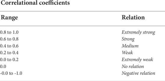
TABLE 1. Pearson’s correlational coefficient variables.

Correlation analysis was performed on the data from 1 January 2010, to 31 December 2014. This dataset consists of different variables, such as, “the hourly temperature (Tem), wind speed (WS), relative humidity (RH), precipitation (Pr) and solar radiation (SR), air pressure (AP), and the actual load demand (LD)”. There are several extremely interesting observations to be made, as explained in Section 4.1.

3 Proposed methodology

Deep residual networks (deep-ResNet) are the foundation of our model for day-ahead load forecasting, which we presented in this study. We begin by formulating the low-level fundamental structure of the model, which consists of numerous layers that are all completely related to one another, and process the inputs of the model to create tentative predictions for the next 24 hours. After then, the preliminary projections are processed by a comprehensive residual network. Following the presentation of the topology of the ResNet, many adjustments are done in order to further improve its capacity for learning.

3.1 Deep neural networks

Deep Neural Networks (DNNs) are ANNs with numerous hidden layers between the input layer and the output layer Ma (2021). The linear and non-linear associations between data characteristics are modelled by using DNN. In modeled, the propensity to overfit may be mitigated by using dropout, a technique in which neurons are removed from the network in either a random or a systematic manner Salinas et al. (2020). Since their inception, DNNs have made significant achievements in a wide range of areas of study. According to Subbiah and Chinnappan (2020), the field of deep learning exploded after their original publication was released in 2006. Through the use of the summation and product procedures, the non-linear function that effectively represents the data is determined in the neural networks. Figure 1 depicts an ANN-based DNN structure. There are three layers in the DNN: an input layer, a hidden layer, and an output layer. Each layer is made up of neurons that do not communicate with each other. There are, nevertheless, complete weighted connections between neurons between layers. The fundamental formulae of DNN in classic networks are as follows;

$y_{\mathit{output}}=F\left(x_{\mathit{input}}\right)(2)$

FIGURE 1

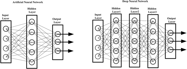
FIGURE 1. The structure of ANN-based DNN.

Where the input of the neuron is denoted by x_input and the output of the neuron is denoted by y_output.

DNNs are able to extract highly abstracted characteristics from training data because of their multiple hidden layers, which provide this power. Since load profiles include nonlinear features among the different components that determine the morphologies of load patterns, it is possible to use DNN as a prediction model under these circumstances. However, the DNNs have two problems when they are being trained to do a task: gradient explosion/vanish and network degeneration.

3.2 Deep residual networks

The aforementioned model is used in order to discover the nonlinear connection that exists between the input data and the output value. In general, the neural network’s learning capacity improves as the model depth is increased. However, there is a possibility that the performance of the deep learning model would suffer in reality. The inherent quality of the data or the challenging nature of the deep learning model might both be to responsible for the deteriorating performance. For greater performance, Zhang et al. (2018) presented an approach that used ResNet instead of stacking concealed layers. ResNet has a unique structure in comparison to nested layers. It is essentially the same as the framework suggested in Zhang et al. (2021), which is often employed for the picture/image classification issue but with a few key differences. In the ResNet building block, the skip link/connection typically has input and output dimensions that are the same, but in a residual block, the input (x_input) and output (y_output) dimensions are different. A ResNet, as seen in Figure 2, has two stacked levels and one skip link/connection.

FIGURE 2

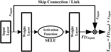
FIGURE 2. The basic structure of Residual Network (ResNet).

Typically, a skip connection is an identical mapping when its input and output are of the same dimension. For this case, the output of the appropriate ResNet is as follows:

$y_{\mathit{output}}=F\left(x_{\mathit{input}}\right)+x_{\mathit{input}}(3)$

If the dimensions of the input and output are not the same, then the skip connection act as a linear projection. In this case, the associated ResNet produces an output with linear projection (L_p) as follows:

$y_{\mathit{output}}=F\left(x_{\mathit{input}}\right)+L_p\ast x_{\mathit{input}}(4)$

The skip connection signifies that the ResBlock/ResNet learning ability is no weaker than that of the stacked layers when both have the same number of hidden layers. The formula for forward-propagation if n residual blocks are formed one after the other is given as follows:

$y\left(x\right)=x_{\mathit{initial}}+\sum _{j=1}^{n}F\left(x_j-1\right)(5)$

Where x_initial represents the very first input that the network receives. In point of fact, the residual block builds an artificial identity map by performing an addition that combines the input and output of the neural unit in a straightforward manner. Experiments have shown that the residual block is an effective solution to the issue of deterioration that occurs in DNNs. Sheng et al. (2021), explained the residual block, both from the point of view of advancing propagation and backward propagation [30].

3.3 A modified structure of deep residual network

The proposed model is presented in this subsection; it is based on the model structure shown in Figure 2. As a result of its design, the proposed model can learn both deep and superficial characteristics or features from the input data that is fed into it. Furthermore, the ResBlocks structure enables that the modified deep-ResNet learning capacity is equivalent to that of a shallow ResNet. According to Zhang et al. (2018), there is a way to expand the deep-ResNet by adding more shortcuts. Although the formulations of the forward and backward propagation of responses and gradients are somewhat different, the network features are the same after adding the additional shortcut links. In order to enhance ResNet learning capacity, we make structural changes to the network. The convolutional network designs suggested in Chen et al. (2019) and Kondaiah and Saravanan (2021) served as inspiration for our proposal of the modified deep-ResNet, the structure of which is seen in Figure 3.

FIGURE 3

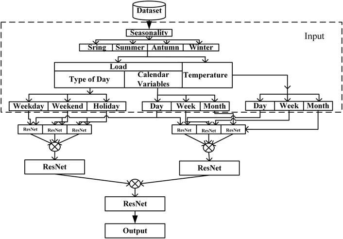
FIGURE 3. The Proposed Structure of a modified deep-ResNet.

A sequence of ResNets is added to the model first (the residual blocks on the right). The input of both side residual blocks is the combination of load values regarding the calendar variables with day type, and the temperature information, respectively, unlike the implementation in Xu et al. (2020) (except for the first side residual block, whose input is the input of the network). This layer output is averaged across the outputs of each of the primary residual blocks. Then the outputs are linked to all of the major remaining blocks in the following layers, much like the tightly connected network in Li Z. et al. (2021). After averaging all connections from the blocks on the right and the network output, the following major residual block is provided as an input. As a result of the extra side residual blocks and dense shortcut connections, it is anticipated that the network representation capabilities and error back-propagation efficiency would increase. In the next section of this study, we will evaluate and contrast the performance of the proposed model.

4 Results and discussion

The proposed model in this experiment is trained by the Adam optimizer with default parameters, as mentioned in Kondaiah and Saravanan (2021). The models are accomplished by adopting Keras 2.2.4 with Tensorflow 1.11.0 as the backend in the Python 3.6 environment. Note that adaptive adjustment of the learning rate during the training process is used. The models are trained on an Intel(R) Core(TM)- i5-3230M-powered Acer laptop. Moreover, the generalizability of the developed model was investigated in two case studies with IESO-Canada and ISO-NE datasets, respectively. Finally, the proposed model performance was verified using real-time data. To train the model, 3 years of data were used, which was taken around 1.5 h for 700 epochs. When training all models, the total training duration is under 8 hours. “Mean absolute percentage error (MAPE), Root mean square error (RMSE), and Mean absolute error (MAE)” are the most significant indices when comparing the results of various STLF models Li et al., 2016b. They are described as follows:

$MAPE=\frac{1}{N}\sum _{n=1}^N\left(\left|\frac{Loa{d}_{Actua{l}_n-Loa{d}_{Predicte{d}_n}}}{Loa{d}_{Actua{l}_n}}\right|\ast 100\right)(6)$

$RMSE=\sqrt{\frac{1}{N}\sum _{n=1}^N{\left(Loa{d}_{Actua{l}_n}-Loa{d}_{Predicte{d}_n}\right)}^2}(7)$

$MAE=\frac{1}{N}\sum _{n=1}^N\left|Loa{d}_{Actua{l}_n}-Loa{d}_{Predicte{d}_n}\right|(8)$

Where N is the total number of input values,$Loa{d}_{Actua{l}_n}$ and $Loa{d}_{Predicte{d}_n}$ are the average values of the actual and predicted load, respectively.

4.1 Analysis of input data

4.1.1 Data pre-processing

The gathered dataset(s) may have multiple anomalies, including missing values, incomplete data, noises, and raw format Shi et al. (2018). The unprocessed data contains flaws and contradictions that might lead to misunderstanding and indicate a lack of proper data analysis. Therefore, the pre-processing stage that is part of the data refining process is particularly crucial for real-world datasets since it ensures the performance and reliability of the system to find information from real-world data. In most cases, the pre-processing data stage consists of many fundamental sub-steps or phases that are applied to raw data before they are refined. These phases and sub-steps are as follows: 1) Data-Cleaning, 2) Data-Transformation, 3) Data-Reduction, 4) Data- Discretization, respectively. These stages are primarily employed in the pre-processing step to improve and evaluate data in order to efficiently and accurately anticipate. As a result, a variety of sub-phases may be effectively used based on the data format, strategy, and input requirements for the suggested methodology.

4.1.2 Description of the data

Two different public data sets are utilized in this work, both of which contain hourly load and weather related data. The first dataset is New England’s independent system operator (ISO-NE)² dataset Chen et al. (2019). The time range of this dataset is from March 2003 to December 2014. The second dataset is Canada’s Independent Electricity System Operator (IESO)³ dataset El-Hendawi and Wang (2020). The time scope of this dataset is from 1st January 2002 to 12th November 2021. These datasets are time series, which are taken into account in minutes, hours, or even days. Trend, cycle, seasonal variation, and erratic fluctuations are the most common features of time series data. In a time series context, a trend is an upward and downward movement that depicts the long-term advancement or deterioration. “Cycle” refers to the periodic oscillations that take place around a trend level. In time series, seasonal variation refers to the recurrence of time interval patterns that complete themselves inside a year’s calendar and reoccur annually. Any movement in a time series that does not follow the regular pattern, known as an irregular variation, is unforeseen and unexpected. For example, the data that we collected for the load in the case study is presented as a time series that is denoted by the hour, as depicted in Figure 4.

FIGURE 4

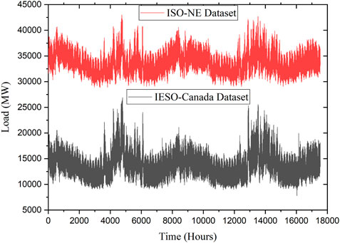
FIGURE 4. Time-Series load data from the two-utility dataset.

The 2-year load demand of both utilities is shown graphically in Figure 4. As seen in Figure, the ISO-NE grid data shows a repeating and cyclic load pattern. In addition to that, the seasonal fluctuation may be noted as well. Nevertheless, the shape of the curve remains the same throughout each year. Furthermore, the IESO data also has the same repeating and cyclic load pattern. This indicates that the load data are subject to annual and seasonal changes. Additionally, the characteristics of load data are as follows. From the hourly load demand as shown in Figure 4; observation reveals that the daily, weekly, and annual patterns represent the most significant seasonal components of load demand. Furthermore, daily load characteristics exhibit a distinct seasonality pattern due to the same fluctuations in load demand as the delayed load variables for seasonal components. In terms of weekday consumption patterns, there is a lot of overlap with weekend consumption patterns. In addition, the workday has a more prominent peak demand than the weekend. And also, the public holidays are characterised by a high demand for electricity on weekends and special days. On the other hand, the everyday power consumption is equivalent to that of a special day. Due to various anthropogenic activities, such as public sector celebrations and festivities, the demand for power increases. There is a significant seasonal variation in the amount of power used. Therefore, the observation results reveal that the lagged load parameters exhibited a substantial correlation and seasonal dependence on the actual load.

4.1.3 Inputs selection for the model

As mentioned earlier the datasets consist of different variables. The correlation analysis was performed on the input data by using Eq. 1. As a result, there are several extremely interesting observations to be made, as seen in Figure 5.

FIGURE 5

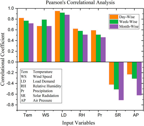
FIGURE 5. Correlational Analysis between the input variables.

Among the several climatic factors that affect electrical load, the temperature is the one that has the most extraordinary sensitivity. The warmer it is throughout the summer months (June, July, and August), the greater the electrical grid demand is expected. So, a positive relationship exists respectively between the actual load and temperature. There is a negative correlation between actual load and the relative humidity in the winter months (December, January, February) and a positive correlation in other months (June to September). This may be due to the fact that the heating load is reduced in winter. At the same time, the warming in summer increases load consumption for air conditioners and other electrical-related machinery for cooling purposes. There will be large increases in the power consumption utilised for heating during the chilly winter with high relative humidity; summer precipitation has a considerable negative association with the actual load; because precipitation cools the weather and reduces the need for refrigeration, this may be the reason. In the winter and summer, wind speed has an opposing influence on load; the temperature may have dropped because of the strong wind. As heating loads rise in the winter, air conditioners and fans must work harder, whereas cooling loads fall in the summer. In all seasonal months, solar radiation and air pressure have negligible influence on load; several research studies are confident that forecasting performance may be enhanced by eliminating factors with marginal correlation with load demand Zhang and Guo (2020). Because of the low correlation between SR and AR, only the hourly-based (h)-Tem, WS, RH, and Pr were selected as inputs for load forecasting in this study. These are all listed in Table 2.

TABLE 2

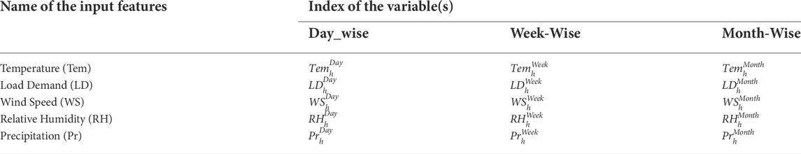
TABLE 2. Input Features for the model.

From the perspective of several research works, special days⁴, seasonality, and normal working days have somewhat distinct load series characteristics. For example, enhancing predicting accuracy may be achieved by using separate systems for special days and normal workdays Song et al., 2005; Fidalgo and Peças Lopes, 2005[35,36]. For this consequence, dummy variables were implemented (see Table 3) in order to partition the data set into three distinct subgroups.

TABLE 3

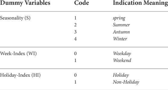
TABLE 3. Additional input variables for the model.

4.1.4 Performance analysis of the proposed model

4.1.4.1 Case study 1: With ISO-NE dataset

The first case study uses the ISO-NE utility dataset. This dataset from the New England utility contains previous load and weather variables at a 1-h resolution. Also, it covers data between 1st March 2003 and 31st December 2014. Furthermore, this case study is concerned with estimating the load for the year 2006. Therefore, the complete details of the input, training, and test data required for the proposed model are as follows to achieve this objective.

The 2 years earlier to 31st December 2014, are utilised as the test set and the training set. To be more explicit, there are two beginning dates that are utilised for the training sets. These starting dates are the first of March 2004 and the first of January 2010. We adjust the hyper-parameters by utilising the last ten percent of the training set that contains this beginning date since it is revealed in studies that are published in the literature. The hyper-parameters are the same for the model that was trained with 2 years of extra data.

ResNet is adopted for the proposed model, and then each residual block is constructed with a hidden layer that has 20 nodes and typically uses an activation function as SELU⁵. The block outputs have the same 24 elements size as their respective inputs. Such a way that, the proposed network consisting of sixty layers is created by stacking a total of thirty residual blocks. Five different models are trained for each implementation with 600, 650, and 700 epochs respectively.

If we look at the contrast of the proposed model with others, the day-based wavelet neural network (SIWNN) model shown in reference Chen et al. (2010) is trained using data from 2003 to 2005, whereas the models presented in references Li et al., 2016b, Li et al. (2016a), and Chen et al. (2019) utilise data from March 2003 to December 2005 for their training. The month-wise proposed model MAPE findings are shown in Table 4. There is no specific reporting of the MAPEs for the whole year 2006 in reference number Li et al., 2016b. As is evident from the information shown in the Table, the suggested model has the lowest MAPE throughout the year 2006. Despite this, we are able to draw the conclusion that the proposed model is capable of high generalisation across a variety of datasets since the majority of the hyper-parameters are not adjusted using the ISO-NE dataset.

TABLE 4

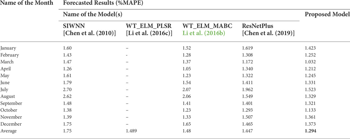
TABLE 4. The month-wise estimation results (% MAPE) of the proposed model with other model(s) on the ISO-NE dataset.

Using data from 2010 to 2011, we further evaluate the proposed model generalisation capabilities. In this scenario, we used the same model developed for the year 2006 and train it using data collected between 2004 and 2009. The results of the proposed model are summarized in Table 5 and compared with the results of the other models discussed in Yu et al., 2014, Cecati et al (2015), and Li et al (2016c), Chen et al (2019). According to the obtained results, the suggested deep-ResNet model performs better than the already available models in terms of the total MAPE for both years It is significant to note that the proposed model is implemented without even additional tuning, while all previous models were tuned using the ISO-NE dataset during the period of 2004–2009.

TABLE 5

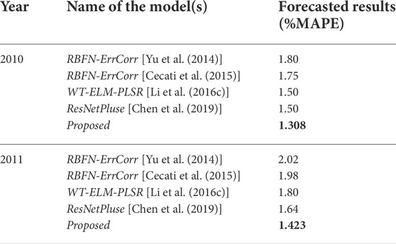
TABLE 5. Year-Wise forecasted results (%MAPE) of the proposed model with other model(s) on the ISO-NE dataset.

Furthermore, the proposed model generalization capabilities were investigated on the load estimation in weekday/end(s) and holiday(s) wise during the years 2006,2010, and 2011 respectively. For this case, we used the same model developed for estimating the load of the year 2006. The suggested model results are summarised in Table 6 and Tables 7. However, the suggested model has slightly different MAPE values in the results of the year 2010. The reason may be the model was confused while at the training period due to the variance in the data. From these results, the suggested model performs better in estimation and has minimal MAPE. It is significant to note that the proposed model is implemented without even additional tuning.

TABLE 6

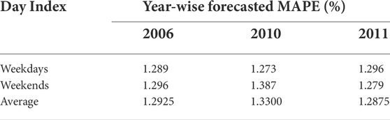
TABLE 6. Day-wise forecasted results (%MAPE) of the model on the ISO-NE dataset.

TABLE 7

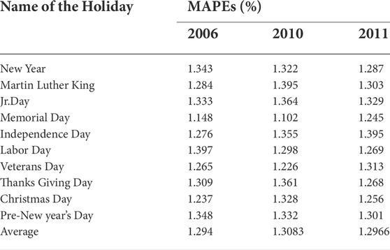
TABLE 7. Holiday(s)-wise forecasted results (%MAPE) of the model on the ISO-NE dataset.

4.1.4.2 Case study 2: With IESO-Canada dataset

The secondary intention of this research is to investigate the generalizability of the developed model. For this purpose, we train the prediction model with the IESO-Canada dataset by adopting the significant number of the hyper-parameters of deep-ResNet optimized for the New England utility dataset. Take into consideration that the methodology utilized here is quite similar to case Study 1. This case study’s primary goal is to forecast 2006s load like the prior scenario. As a result, the training set consists of data collected before 12 November 2021, while the test set consists of data collected 2 years before that date.

In Table 8, we validated the performance of the proposed model with that of the models presented in El-Hendawi and Wang (2020) and Kondaiah and Saravanan (2022). From the information shown in the table, it can conclude that the suggested model is more effective than the other prediction models. In addition to being more efficient than competing models, the presented model has less MAPE. If additional data is supplied to the training set, the model test loss may be decreased even more.

TABLE 8

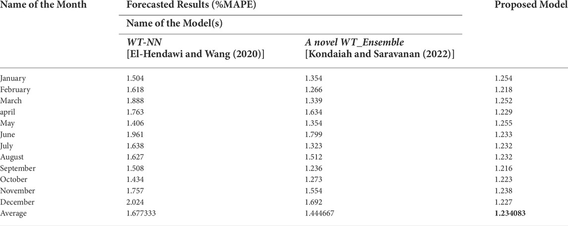
TABLE 8. The month_wise estimation results (% MAPE) of the proposed model with other model(s) on the IESO-Canada dataset.

4.1.4.3 Case study 3: Testing of the proposed model using real-time data

In this context, to verify the proposed model using real-time data, we have forecasted the load for the next day from the IESO-Canada utility dataset. For this purpose, the model was trained and tested with the data taken from the same dataset as per the procedure followed in the second case study. Furthermore, a significant number of hyper-parameters were adopted by the optimized model in that same case study. As result, the forecasted and actual load for 2nd August 2022 was shown in Figure 6, and the (%) MAPE is only 1.19045.

FIGURE 6

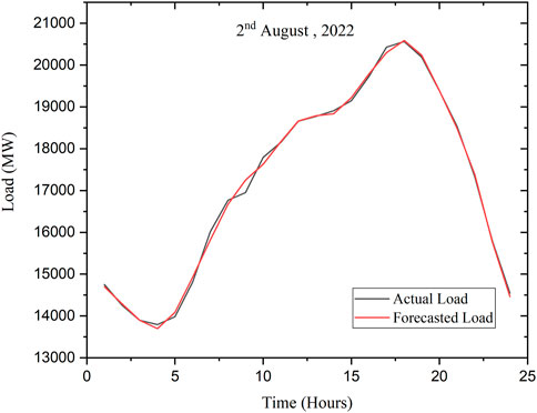
FIGURE 6. The forecasted and actual load for 2nd August 2022.

5 Conclusion

A model for STLF based on a modified version of a DNN was suggested in this paper. By utilizing a statistical correlation approach, the appropriate inputs to the model were chosen. The efficacy of the proposed model was evaluated with different test scenarios on the ISO-NE and IESO-Canada utility datasets. The suggested model has been proved to be better regarding the accuracy of its forecasts based on comparisons with other models already in existence.

The MAPE (%) using the modified deep-ResNet method for ISO-NE data is 1.294, which is comparatively less to other models available in the literature. Simillarly, the MAPE (%) for IESO-Canada data is 1.234083, which is also less and the same is represented in Table 8. These results shows the effectiveness of the proposed model (deep-ResNet). Also, in case 3, the model was tested with real-time data, and the error MAPE is 1.19045%

There is still a considerable amount of work to be done as future work. We have considered the basis of the possibility of DNNs here, but there are probably many different architectures of these networks that could be combined with the model to improve its performance. However, it is also possible to explore further research on the technique of probabilistic load forecasting with DNN. Additionally, the model accuracy can be improved by considering a more significant number of meteorological factors.

Data availability statement

The raw data supporting the conclusions of this article will be made available by the authors, without undue reservation.

Author contributions

VK has analyzed and implemented the STLF application methodology in the smart grid environment. And also prepared the original manuscript. BS has supervised the work and reviewed/edited the manuscript. VK and BS have conceptualized, validated, and investigated.

Conflict of interest

The authors declare that the research was conducted in the absence of any commercial or financial relationships that could be construed as a potential conflict of interest.

Publisher’s note

All claims expressed in this article are solely those of the authors and do not necessarily represent those of their affiliated organizations, or those of the publisher, the editors and the reviewers. Any product that may be evaluated in this article, or claim that may be made by its manufacturer, is not guaranteed or endorsed by the publisher.

Footnotes

¹such as temperature, relative humidity, wind speed, and precipitation.

²https://class.ee.washington.edu/555/el-sharkawi.

³http://reports.ieso.ca.

⁴Saturday, Sunday, holidays.

⁵Scaled exponential linear unit.

References

Ali, M., Adnan, M., Tariq, M., and Poor, H. V. (2021). Load forecasting through estimated parametrized based fuzzy inference system in smart grids. IEEE Trans. Fuzzy Syst. 29, 156–165. doi:10.1109/TFUZZ.2020.2986982

CrossRef Full Text | Google Scholar

Amarasinghe, K., Marino, D. L., and Manic, M. (2017). Deep neural networks for energy load forecasting. IEEE Int. Symposium Industrial Electron. doi:10.1109/ISIE.2017.8001465

CrossRef Full Text | Google Scholar

Bento, P. M., Pombo, J. A., Calado, M. R., and Mariano, S. J. (2019). Optimization of neural network with wavelet transform and improved data selection using bat algorithm for short-term load forecasting. Neurocomputing 358, 53–71. doi:10.1016/j.neucom.2019.05.030

CrossRef Full Text | Google Scholar

Cecati, C., Kolbusz, J., Rózycki, P., Siano, P., and Wilamowski, B. M. (2015). A novel RBF training algorithm for short-term electric load forecasting and comparative studies. IEEE Trans. Ind. Electron. 62, 6519–6529. doi:10.1109/TIE.2015.2424399

CrossRef Full Text | Google Scholar

Chen, K., Chen, K., Wang, Q., He, Z., Hu, J., and He, J. (2019). Short-term load forecasting with deep residual networks. IEEE Trans. Smart Grid 10, 3943–3952. doi:10.1109/TSG.2018.2844307

CrossRef Full Text | Google Scholar

Chen, Y., Luh, P. B., Guan, C., Zhao, Y., Michel, L. D., Coolbeth, M. A., et al. (2010). Short-term load forecasting: Similar day-based wavelet neural networks. IEEE Trans. Power Syst. 25, 322–330. doi:10.1109/TPWRS.2009.2030426

CrossRef Full Text | Google Scholar

Chitalia, G., Pipattanasomporn, M., Garg, V., and Rahman, S. (2020). Robust short-term electrical load forecasting framework for commercial buildings using deep recurrent neural networks. Appl. Energy 278, 115410. doi:10.1016/j.apenergy.2020.115410

CrossRef Full Text | Google Scholar

El-Hendawi, M., and Wang, Z. (2020). An ensemble method of full wavelet packet transform and neural network for short term electrical load forecasting. Electr. Power Syst. Res. 182, 106265. doi:10.1016/j.epsr.2020.106265

CrossRef Full Text | Google Scholar

Ferraty, F., Goia, A., Salinelli, E., and Vieu, P. (2014). “Peak-load forecasting using a functional semi-parametric approach,” in Springer proceedings in mathematics and statistics. doi:10.1007/978-1-4939-0569-0_11

CrossRef Full Text | Google Scholar

Fidalgo, J. N., and Peças Lopes, J. A. (2005). Load forecasting performance enhancement when facing anomalous events. IEEE Trans. Power Syst. 20, 408–415. doi:10.1109/TPWRS.2004.840439

CrossRef Full Text | Google Scholar

Hernández, L., Baladrón, C., Aguiar, J. M., Carro, B., Sánchez-Esguevillas, A., and Lloret, J. (2014). Artificial neural networks for short-term load forecasting in microgrids environment. Energy 75, 252–264. doi:10.1016/j.energy.2014.07.065

CrossRef Full Text | Google Scholar

Hippert, H. S., Pedreira, C. E., and Souza, R. C. (2001). Neural networks for short-term load forecasting: A review and evaluation. IEEE Trans. Power Syst. 16, 44–55. doi:10.1109/59.910780

CrossRef Full Text | Google Scholar

Jiao, R., Zhang, T., Jiang, Y., and He, H. (2018). Short-term non-residential load forecasting based on multiple sequences LSTM recurrent neural network. IEEE Access 6, 59438–59448. doi:10.1109/ACCESS.2018.2873712

CrossRef Full Text | Google Scholar

Kaiming, H., Xiangyu, Z., Shaoqing, R., and Jian, S. (2015). Deep residual learning for image recognition. Proc. IEEE Comput. Soc. Conf. Comput. Vis. Pattern Recognit.

Google Scholar

Kim, W., Han, Y., Kim, K. J., and Song, K. W. (2020). Electricity load forecasting using advanced feature selection and optimal deep learning model for the variable refrigerant flow systems. Energy Rep. 6, 2604–2618. doi:10.1016/j.egyr.2020.09.019

CrossRef Full Text | Google Scholar

Kondaiah, V. Y., Saravanan, B., Sanjeevikumar, P., and Khan, B. (2022). A review on short-term load forecasting models for micro-grid application. J. Eng. 202, 665–689. doi:10.1049/tje2.12151

CrossRef Full Text | Google Scholar

Kondaiah, V. Y., and Saravanan, B. (2022). Short-term load forecasting with a novel wavelet-based ensemble method. Energies 15, 5299. doi:10.3390/en15145299

CrossRef Full Text | Google Scholar

Kondaiah, V. Y., and Saravanan, B. (2021). “Short-term load forecasting with deep learning,” in 3rd IEEE international virtual conference on innovations in power and advanced computing technologies. i-PACT 2021. doi:10.1109/i-PACT52855.2021.9696634

CrossRef Full Text | Google Scholar

Kong, W., Dong, Z. Y., Jia, Y., Hill, D. J., Xu, Y., and Zhang, Y. (2019). Short-term residential load forecasting based on LSTM recurrent neural network. IEEE Trans. Smart Grid 10, 841–851. doi:10.1109/TSG.2017.2753802

CrossRef Full Text | Google Scholar

Kuster, C., Rezgui, Y., and Mourshed, M. (2017). Electrical load forecasting models: A critical systematic review. Sustainable Cities and Society. 35. 257-270. doi:10.1016/j.scs.2017.08.009

CrossRef Full Text | Google Scholar

Kwon, B. S., Park, R. J., and Song, K. B. (2020). Analysis of the effect of weather factors for short-term load forecasting. Transactions of the Korean Institute of Electrical Engineers. 69. Seoul, Korea. 985-992. doi:10.5370/KIEE.2020.69.7.985

CrossRef Full Text | Google Scholar

Li, C., Liang, G., Zhao, H., and Chen, G. (2021a). A demand-side load event detection algorithm based on wide-deep neural networks and randomized sparse backpropagation. Front. Energy Res. 9. doi:10.3389/fenrg.2021.720831

CrossRef Full Text | Google Scholar

Li, J., Sun, A., Han, J., and Li, C. (2022). A survey on deep learning for named entity recognition. IEEE Trans. Knowl. Data Eng. 34, 50–70. doi:10.1109/TKDE.2020.2981314

CrossRef Full Text | Google Scholar

Li, S., Goel, L., and Wang, P. (2016a). An ensemble approach for short-term load forecasting by extreme learning machine. Appl. Energy 170, 22–29. doi:10.1016/j.apenergy.2016.02.114

CrossRef Full Text | Google Scholar

Li, S., Wang, P., and Goel, L. (2016b). A novel wavelet-based ensemble method for short-term load forecasting with hybrid neural networks and feature selection. IEEE Trans. Power Syst. 31, 1788–1798. doi:10.1109/TPWRS.2015.2438322

CrossRef Full Text | Google Scholar

Li, Z., Li, Y., Liu, Y., Wang, P., Lu, R., and Gooi, H. B. (2021b). Deep learning based densely connected network for load forecasting. IEEE Trans. Power Syst. 36, 2829–2840. doi:10.1109/TPWRS.2020.3048359

CrossRef Full Text | Google Scholar

Liu, D., Zeng, L., Li, C., Ma, K., Chen, Y., and Cao, Y. (2018). A distributed short-term load forecasting method based on local weather information. IEEE Syst. J. 12, 208–215. doi:10.1109/JSYST.2016.2594208

CrossRef Full Text | Google Scholar

Liu, Z., Li, W., and Sun, W. (2013). A novel method of short-term load forecasting based on multiwavelet transform and multiple neural networks. Neural computing and applications. 22. 271–277. doi:10.1007/s00521-011-0715-2

CrossRef Full Text | Google Scholar

Ma, S. (2021). A hybrid deep meta-ensemble networks with application in electric utility industry load forecasting. Inf. Sci. 544, 183–196. doi:10.1016/j.ins.2020.07.054

CrossRef Full Text | Google Scholar

Memarzadeh, G., and Keynia, F. (2021). Short-term electricity load and price forecasting by a new optimal LSTM-NN based prediction algorithm. Electr. Power Syst. Res. 192, 106995. doi:10.1016/j.epsr.2020.106995

CrossRef Full Text | Google Scholar

Rafi, S. H., Al-Masood, N., Deeba, S. R., and Hossain, E. (2021). A short-term load forecasting method using integrated CNN and LSTM network. IEEE Access 9, 32436–32448. doi:10.1109/ACCESS.2021.3060654

CrossRef Full Text | Google Scholar

Salinas, D., Flunkert, V., Gasthaus, J., and Januschowski, T. (2020). DeepAR: Probabilistic forecasting with autoregressive recurrent networks. Int. J. Forecast. 36, 1181–1191. doi:10.1016/j.ijforecast.2019.07.001

CrossRef Full Text | Google Scholar

Sheng, Z., Wang, H., Chen, G., Zhou, B., and Sun, J. (2021). Convolutional residual network to short-term load forecasting. Appl. Intell. (Dordr). 51, 2485–2499. doi:10.1007/s10489-020-01932-9

CrossRef Full Text | Google Scholar

Shi, H., Xu, M., and Li, R. (2018). Deep learning for household load forecasting-A novel pooling deep RNN. IEEE Trans. Smart Grid 9, 5271–5280. doi:10.1109/TSG.2017.2686012

CrossRef Full Text | Google Scholar

Song, K.-b., Baek, Y.-s., Hong, D. H., and Jang, G. (2005). Short-term load forecasting for the holidays using. IEEE Trans. Power Syst.

Google Scholar

Subbiah, S. S., and Chinnappan, J. (2020). An improved short term load forecasting with ranker based feature selection technique. J. Intelligent Fuzzy Syst. 39, 6783–6800. doi:10.3233/JIFS-191568

CrossRef Full Text | Google Scholar

Taylor, J. W. (2010). Triple seasonal methods for short-term electricity demand forecasting. Eur. J. Operational Res. 204, 139–152. doi:10.1016/j.ejor.2009.10.003

CrossRef Full Text | Google Scholar

Velasco, L. C. P., Polestico, D. L. L., Abella, D. M. M., Alegata, G. T., and Luna, G. C. (2018). Day-ahead load forecasting using support vector regression machines. Int. J. Adv. Comput. Sci. Appl. 9. doi:10.14569/IJACSA.2018.090305

CrossRef Full Text | Google Scholar

Wang, Y., Gan, D., Sun, M., Zhang, N., Lu, Z., and Kang, C. (2019). Probabilistic individual load forecasting using pinball loss guided LSTM. Appl. Energy 235, 10–20. doi:10.1016/j.apenergy.2018.10.078

CrossRef Full Text | Google Scholar

Xu, Q., Yang, X., and Huang, X. (2020). Ensemble residual networks for short-term load forecasting. IEEE Access 8, 64750–64759. doi:10.1109/ACCESS.2020.2984722

CrossRef Full Text | Google Scholar

Yu, H., Reiner, P. D., Xie, T., Bartczak, T., and Wilamowski, B. M. (2014). An incremental design of radial basis function networks. IEEE Trans. Neural Netw. Learn. Syst. 25, 1793–1803. doi:10.1109/TNNLS.2013.2295813

PubMed Abstract | CrossRef Full Text | Google Scholar

Zhang, G., and Guo, J. (2020). A novel method for hourly electricity demand forecasting. IEEE Trans. Power Syst. 35, 1351–1363. doi:10.1109/TPWRS.2019.2941277

CrossRef Full Text | Google Scholar

Zhang, K., Sun, M., Han, T. X., Yuan, X., Guo, L., and Liu, T. (2018). Residual networks of residual networks: Multilevel residual networks. IEEE Trans. Circuits Syst. Video Technol. 28, 1303–1314. doi:10.1109/TCSVT.2017.2654543

CrossRef Full Text | Google Scholar

Zhang, Y., Tian, Y., Kong, Y., Zhong, B., and Fu, Y. (2021). Residual dense network for image restoration. IEEE transactions on pattern analysis and machine intelligence. 43. 2480-2495. doi:10.1109/TPAMI.2020.2968521

PubMed Abstract | CrossRef Full Text | Google Scholar

Nomenclature

ANN Artificial Neural Network

CNN Convolutional Neural Network

deep − ResNet Deep Residual Network

DNN Deep Neural Network

ELM Extreme Learning Machine

IESO − Canada Independent Electricity System Operator-Canada

ISO − NE Independent System Operator-New England

LSTM Long Short-Term Memory

MAE Mean Absolute Error

MAPE Mean Absolute Percentage Error

NLP Natural Language Processing

RBF Radial Basis Function

RBM Restricted Boltzmann Machine

ResNet Residual Network

RMSE Root Mean Square Error

STLF Root Mean Square Error

SVR Support Vector Regression