Peak power prediction method of heat pipe cooled reactor start-up and power-up processes based on ANN

1 Introduction

The heat pipe cooled reactor is an advanced solid-state reactor whose core consists of a hexagonal stainless-steel monolith structure containing uranium-oxide (UO₂) fuel pins and heat pipes. As the core heat transfer component, the heat pipes carry away the core heat to the second loop or the thermoelectric conversion device in a non-energetic manner, eliminating pumps, valves, and auxiliary support systems. Hence, unlike traditional light water reactors, heat pipe cooled reactors are characterized by high inherent safety, compact structure, low operation pressure, long core life, and sound economy, and can be applied to particular scenarios such as deep-sea, space, and star surface. However, due to the small delayed neutron fraction, low matrix heat capacity, weak fuel, and matrix Doppler effects in heat pipe cooled reactor, it faces rapid variation in power with reactivity perturbations and temperature fluctuations.

The peak power is an essential factor affecting reactor safety, and reactors are generally designed with over-power protection devices to protect the reactor from over-power. Once the over-power protection signal is triggered, the reactor will shut down urgently. In most application scenarios, heat pipe cooled reactors must operate unattended for an extended period. In the face of load changes, the operating system needs to startup or mediate power to match the reactor power to the load while keeping the peak power in a reasonable range. Considering the rapid power variation of heat pipe cooled reactor, the implementation of this function relies on the accurate and fast prediction of the core power.

The reactor core power is generally obtained by the physical model based on the nuclear reaction mechanism or the analytical method of the experimental model. Dias and Silva (2016) used the neutron flux density method to infer the reactor power. However, the neutron flux density is not only related to the power level but also affected by the degree of fuel consumption. Song (2002) sensors outside the core to measure the power, but it is challenging to arrange sensors in some scenarios. The sensitivities of the sensors will also affect the accuracy of power estimation. Simple mathematical or physical models cannot accurately describe or estimate the nuclear reaction process due to a large number of non-linearities and uncertainties involved.

Numerical simulation of the phenomena in the reactor by coupling the thermohydraulic and neutronics models is another means. Xi et al. (2013) analyzed the axial power distribution of the European supercritical water-cooled reactor SCWR FA by coupling the thermohydraulic code CFX and the neutronics code MCNP. Although the best estimation procedure provides accurate results, it does not meet the requirements for autonomous operation in remote due to a large amount of computation time.

With the development of machine learning techniques, the use of data-driven models to predict the trends of critical parameters in real-time based on the feature parameters plays an increasingly active role in the safe operation of nuclear power plants. Bae et al. (2021) proposed a data-driven model consisting of a multi-step prediction strategy and an artificial neural network, which can help the operators estimate the trend of parameters under emergencies to respond quickly to the current situation.

Given the data-driven model’s excellent performance, this study try to apply it to the field of power prediction. This paper takes MegaPower, a heat pipe cooled reactor designed by Los Alamos National Lab for strategic power supply in remote as the subject (Sterbentz et al., 2017). Firstly, a model based on an artificial neural network to predict the peak power of heat pipe cooled reactor start-up and power-up processes is built. Then ensemble approaches are used to optimize the prediction performance further. After that, the applicability of this model is analyzed. Figure 1 shows the entire analysis flowchart of this article.

FIGURE 1

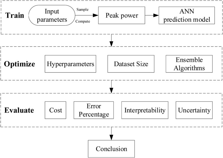
FIGURE 1. The flowchart of the whole analysis process of the neural network prediction model.

2 Problem introduction and dataset

2.1 Problem introduction

MegaPower is a heat pipe cooled reactor designed by Los Alamos National Lab for strategic power supply in remote (Mcclure et al., 2015; Sterbentz et al., 2017). Figure 2 shows some of the major reactor structures.

FIGURE 2

FIGURE 2. Concept schematicof heat pipe cooled reactor MegaPower (Sterbentz et al., 2017).

The core consists of a hexagonal stainless-steel monolith structure containing 5.22 Mt of uranium-oxide (UO₂) fuel pins and liquid metal potassium (K) heat pipes operating at 675°C. By vaporizing the potassium liquid in the heat pipes, the heat pipes remove heat from the monolith; no pumps or valves are needed. Heat is then deposited in the condenser region of the heat pipe. Condenser regions can accommodate multiple heat exchangers. Reaction control is achieved using alumina (Al₂O₃) neutron side reflectors with 12 embedded control drums containing boron-carbide (B₄C) poison arcs.

The heat pipe cooled reactor increases reactivity by rotating the control drum. Zhong et al. (2021) have proposed a “frog-hopping” power control strategy to improve the safety of the heat pipe cooled reactor in the power mediation process. As shown in Figure 3, the system is as follows.

FIGURE 3

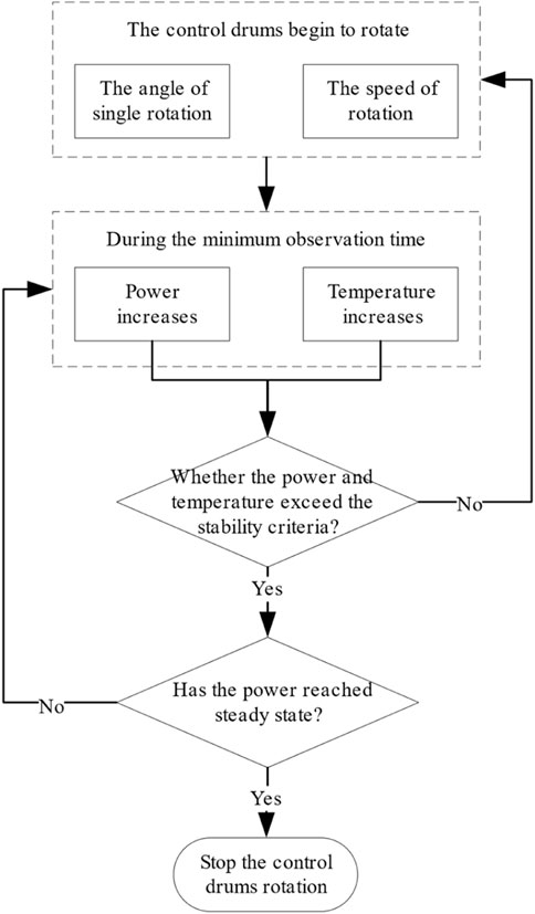
FIGURE 3. Control logic of the control drum.

During the start-up process, when the reactor is critical, after each rotation of the control drum, if the change of the reactor power and the average fuel temperature is within limits during the subsequent observation time, the reactor is considered to be in a controllable state, and the control drum is continued to be rotated. Otherwise, the control drum is stopped until the conditions are satisfied again. In the power-up process, it is necessary to wait some time to perform the following operation after reaching the current power.

Therefore, the main operation parameters affecting the target parameters and their value ranges and distributions were identified, as shown in Table 1. During the process of reaching the target value of the core power, there is an urgent need to know the effect of the parameters on the power, as the different rotation patterns of the control drum may lead to a huge variation of the transient power. Model-based, knowledge-based, and data-driven methods are commonly used for prediction. However, the model-based method has a longer calculation time, the knowledge-based method has little empirical knowledge, and only the data-driven method can overcome the problems in peak power prediction.

TABLE 1

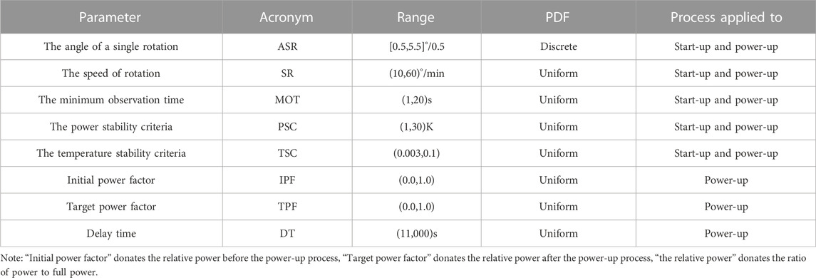
TABLE 1. The range and distribution of the input parameters in start-up and power-up processes.

2.2 Dataset

Although the data-driven method has shown promising applications, its performance is influenced by the quality of the data. In practice, obtaining reliable training data is difficult, which relies on effective procedures. The HPRTRAN is a heat pipe cooled reactor system analysis code developed by the Nuclear Power Institute of China, consisting of a point reactor kinetics model, a reactivity feedback model, a core heat transfer and mechanical model, and a heat pipe model (Ma et al., 2021a).

Figure 4 shows the flowchart of the models in the HPRTRAN code. The neutronic kinetics model determines the total power with the neutron transport simulation to obtain the relative power distribution. Thermal-mechanical calculations are carried out with the transferred power. There are three components to the core multi-channel thermal-mechanical model: a heat pipe model, a single channel coupled thermal-mechanical model, and a radial heat transfer model. Using the heat pipe model, the evaporator outwall temperature and the monolith’s inner wall temperature are determined. By transferring the thermal expansion and temperature distribution from the core thermal-mechanical model to the neutron kinetics model, the reactivity feedback can be considered.

FIGURE 4

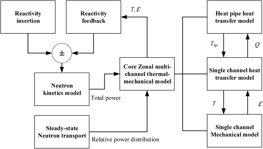
FIGURE 4. Flowchart of the models developed for the transient core analysis in the heat pipe cooled reactor (Ma et al., 2021b).

The reasonability and feasibility of the models were verified by comparing the computational results of the HPRTRAN code with the ANSYS code and experimental results (Ma et al., 2021b; Ma et al., 2022).

HPRTRAN can well simulate the heat pipe reactor in the start-up and power-up processes. Taking the start-up process as an example, the system parameters, including core geometry parameters, power distribution, reactivity feedback, etc., are initialized, followed by transient calculations, where the point kinetic equations, core multi-channel heat transfer model, and heat pipe model are solved explicitly; The core internal reactivity is determined from the fuel, monolith, heat pipe, and reflector operating temperatures, and summed with the external reactivity introduced by the control drum as the total reactivity. Update the temperature field and the heat transfer between channels. Multiple iterations are performed until the preset calculation time is reached. Figure 5 shows the power variation during the start-up process (Ma et al., 2021a).

FIGURE 5

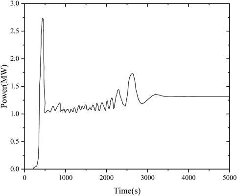
FIGURE 5. The power variation during the start-up process.

As shown in Figure 6, a Monte Carlo simulation is performed for the input parameters of the process of start-up and power-up, respectively. The influence of the input parameters on the target parameters is calculated using HPRTRAN to obtain the dataset containing the input features and the target values. The dataset size for both the start-up and power-up processes is 2000.

FIGURE 6

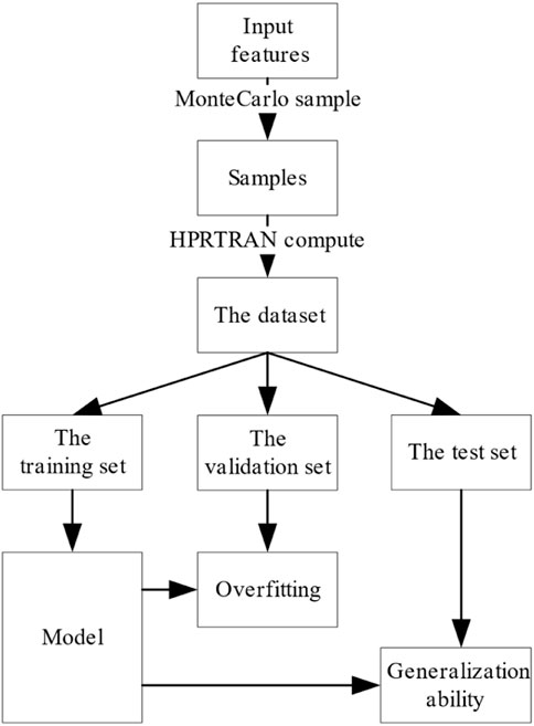
FIGURE 6. Flowchart of the data set calculation in the start-up process and power-up process.

The dataset is divided into a training set, validation set, and test set according to the ratio of 3:1:1. The training set is used to train the prediction model and calculate the model’s parameters. The validation set determines whether the model is underfitting or overfitting. The test set is used to check the model generalization performance.

The model uses the root mean square error (RMSE) between the predicted and actual values of the target parameters as the evaluation metric, as shown in the following equation.

$RMSE=\sqrt{\frac{1}{N}{\displaystyle \sum }_{i=1}^N\left[{\left(f_i^{predict}-f_i^{true}\right)}^2\right]}(1)$

Sobol sensitivity analysis is based on the variance decomposition technique. It is suitable for measuring the non-linear relationship between multiple input parameters and outputs (Ikonen, 2016), selecting a total sensitivity index value of 0.05 as a distinction between important and unimportant parameters (Zhang et al., 2015). Figure 7 shows the Sobol sensitivity index between the input parameters and the target values in the dataset. The results show that although there are differences in the sensitivity indices of each input feature, they satisfy the requirements of the critical parameters, and there are no redundant features.

FIGURE 7

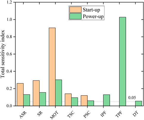
FIGURE 7. Total sensitivity indices between input features and targets of the dataset in the start-up process and power-up process.

3 Regression model

This section introduces the neural network algorithm and three ensemble algorithms.

3.1 Neural network

The neuronal action potential will change when a stimulus is delivered to a neuron in the human brain. If the potential exceeds a threshold, the neuron is activated and sends neurotransmitters to other neurons. The artificial neural network (ANN) is built concerning the structure of the human brain nervous system. The M-P neuron shown in Figure 8 simulates the neuron in the human brain. The M-P neuron receives the input $x_i$ from other neurons, multiplies it by the connection weight ${\omega }_i$, and then subtracts the activation threshold $\theta$ to obtain the output value $\sum {\omega }_i{x}_i-\theta$. The non-linear activation function $f$ transforms the original output value to consider the non-linear factor.

FIGURE 8

FIGURE 8. Concept schematicof the M-P neuron model.

As shown in Figure 9, the artificial neural network consists of an input layer, several hidden layers, and an output layer. Each layer includes several M-P neurons. The data are propagated backward and forward, but no co-layer and cross-layer propagation occur.

FIGURE 9

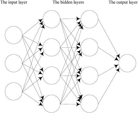
FIGURE 9. Concept schematic of the fully connected artificial neural network model.

The neural network optimizes the parameters $\omega$ and $\theta$ of the neurons using the error back propagation algorithm (BP). The BP algorithm updates the parameters through stochastic gradient descent and can step out of the local optimum values and find the optimum global value.

4.2 Model evaluation

This section provides a comprehensive evaluation of the neural network prediction model in terms of cost, accuracy, interpretability, and uncertainty.

4.2.1 Cost

The artificial neural network has many parameters. There are corresponding connection weights between neurons of adjacent two layers and thresholds on each. The artificial neural network adopts the BP algorithm to update parameters, which requires the input to be propagated layer by layer from front to back. Then the error is propagated step by step from back to front. Ittakes a long time to train the artificial neural network model. Table. 2 shows the time required to prepare and predict the neural network model on the two datasets.

TABLE 2

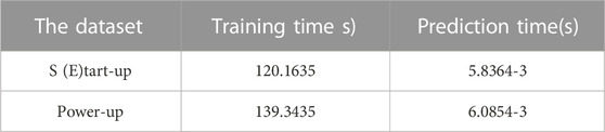
TABLE 2. Training and prediction time of the neural network model.

The complexity of the neural network model is also reflected in the size of the model hyperparameters. Table. 3 shows part of the hyperparameters of the neural network.

TABLE 3

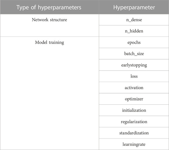
TABLE 3. Partial hyperparameters of the neural network.

The model’s generalization performance can be driven to the best state by adjusting the values of hyperparameters. Due to a large number of hyperparameters, it usually takes time to adjust the parameters of the neural network. Thus, it is more sensible to select the random sampling method in tuning the neural network model.

4.2.2 Error percentage

The peak powers of the test set were predicted using the optimized neural network model, and the error percentage distributions are shown in Figure 10.

FIGURE 10

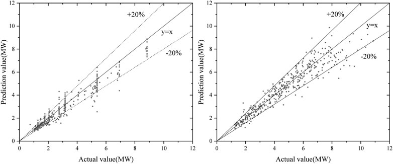
FIGURE 10. Error percentage distribution of test set prediction by the neural network during the start-up process and power-up process.

The error percentages of the neural network are within 20% in both the start-up and the power-up processes, showing the high accuracy of artificial neural networks. There are two reasons. One is that the neural network has lots of parameters that can fit complex functional relations. Hornik (1991) has proved that, under certain conditions, the artificial neural network is capable of arbitrarily accurate approximation to a function. Secondly, in updating the model parameters, the neural network uses the stochastic gradient descent algorithm; it can jump out of the local extremes and find the global minimum.

4.2.3 Interpretability

Talking about the interpretability of models, an eural network is more of a black box in that it delivers results without an explanation. It is only possible to observe what caused the neuron’s activation on the first hidden layer and what the neuron’s activation did on the last hidden layer. It is difficult to understand more neurons in the hidden layers in the middle. Therefore, the neural network is unsuitable for some scenarios requiring high interpretability.

The interpretability of neural networks is currently a research hotspot, which can be divided into active and passive interpretability studies according to whether interpretability interventions are made in the design and training processes of the model. Active interpretation drives neural network models in the direction of interpretability by adding physical information to the structure of the model, using physical constraints in the model’s training process, or combining the neural network with other models with high interpretability. Wan et al. (2020) constructed the neural-backed decision tree NBDT by replacing each node in the decision tree with a neural network, claiming it preserves the high precision of a neural network and high-level interpretability of a decision tree and successfully applied in the field of image recognition. However, due to the specific modification of the internal structure of the neural network by active interpretation, it is less intuitive in interpretation and has a narrow scope of application. Therefore, more work is currently focused on passive interpretation.

In this section, the neural network prediction models are interpreted using the attribution interpretation and the distance interpretation, respectively, according to the decreasing interpretability completeness.

4.2.3.1 Attribution interpretation

The concept of attribution interpretation refers to the attribution of responsibility or blame based on the effects of the input features on the output. The rapid rotation of the control drum brings about a rapid rise in core temperature and the following negative temperature feedback, so the total reactivity fluctuates violently near the criticality, generating power fluctuations and the maximum peak power.

Figure 7 shows the contribution of the input features to the peak power, during the start-up process, with the minimum observation time having the most significant effect on the peak power, followed by the control drum’s angle of a single rotation and speed of rotation. At the microscopic level, the single rotation angle and rotation speed of the control drum directly affect the speed of each control drum rotation. Thus, the contribution to the peak power is enormous. At the macroscopic level, the minimum observation time determines the length of the single rotation interval of the control drum during the “frog-hopping” start-up. Actually, it controls the overall speed of the control drum during the whole rotation.

In the power-up process, the target power factor becomes the most influential factor on the peak power, which is well understood as it determines the steady-state power level and, naturally, the peak power range above the steady-state power.

The above analysis illustrates the usefulness of analyzing the effect of input features on the peak power according to Figure 7. This section takes the power-up process as an example to perform the attribution interpretation by sampling ten samples from the test set. All the samples are normalized and sorted by the output value. As shown in Table. 4, it is easy to identify the features that contribute most on the peak power when it is small or large. For instance, the small PSC value in sample No. 1 limits the speed of power increase. And the large MOT values in samples No. 2–4 extend therotation interval of control drum. All the above factors reduce the reactivity introduction speed. The large peak powers of samples No.8–10 come from the opposite reason.

TABLE 4

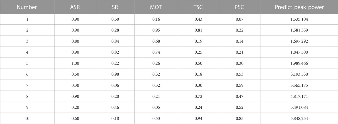
TABLE 4. Attribution interpretation of the peak power prediction model in the power-up process.

The attribution interpretation explains the results from the mechanism, which can deepen the understanding of the peak power formation process, but it requires human confirmation in practice, which is inconvenient. Therefore, this section adopts the distance interpretation method based on Euclidean distance to prove the reliability of the model prediction results.

4.2.3.2 Distance interpretation

The distance interpretation finds the nearest training sample from the training set to explain the output for a particular test sample. A reasonable assumption is that the peak power is considered a function of the input features and that the “derivatives” are present and bounded over most of the domain so that the outputs of the test sample and the nearest training sample should not be too different from each other.

Therefore, this section still selects the above 10 test samples, searches for the nearest training samples and compares their outputs. The results are shown in Figure 11. It is found that the output values of five nearest training samples are within the 20% error range of test samples, indicating that the output of the neural network can be quickly verified by distance interpretation.

FIGURE 11

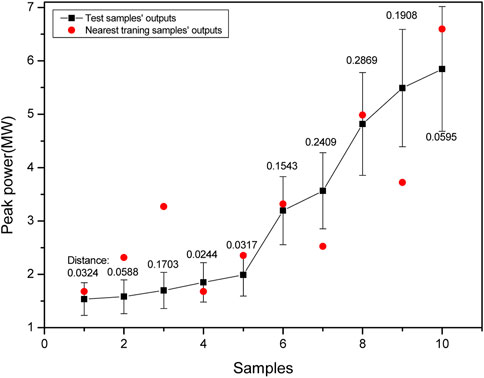
FIGURE 11. Distance interpretation of the peak power prediction model in the power-up process.

4.2.4 Uncertainty

The uncertainty of the model contains epistemic uncertainty and aleatory uncertainty, where the epistemic uncertainty comes from the lack of understanding of the physical system, and aleatory uncertainty comes from the uncertainty of the physical system itself, which is difficult to distinguish in practice. This section analyzes the uncertainty of neural network models by identifying the sources of uncertainty, performing uncertainty propagation, and finally analyzing the output uncertainty.

The uncertainty of neural network comes from the model hyperparameters, training data, and model parameters. The model hyperparameters and training data are controllable uncertainties and can be specified artificially before training. The model parameters are uncontrollable uncertainties, which are updated by the gradient descent method during the training process and cannot be interfered with artificially, so the uncertainty of the model parameters can be considered by adding a Dropout layer to abandon the model parameters randomly (Gurgen, 2021). The process of model uncertainty quantification is shown in the Figure 12.

FIGURE 12

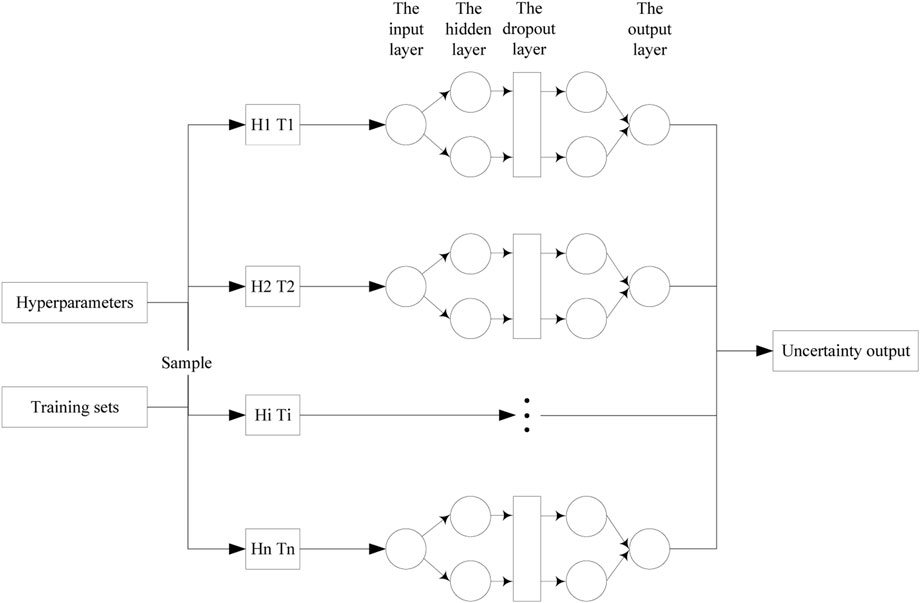
FIGURE 12. The process of uncertainty quantification.

The uncertainty of the model is propagated through the framework shown in Figure 12. And it is then quantified by analyzing the uncertainty output. Taking a sample of the start-up process and the power-up process as an example respectively, the uncertainty outputs of the modelsare shown in Figures 13, 14.

FIGURE 13

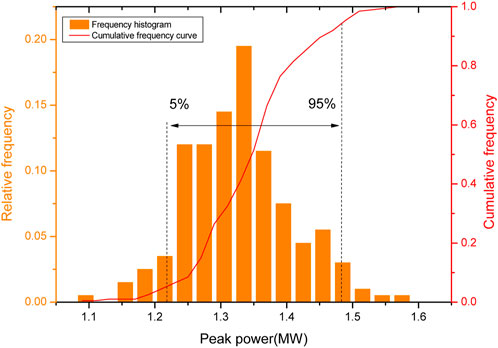
FIGURE 13. Uncertainty quantification of the peak power prediction model in the start-up process.

FIGURE 14

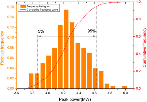
FIGURE 14. Uncertainty quantification of the peak power prediction model in the power-up process.

3.2 Ensemble algorithms

The predictive ability of a regression model for unknown samples is defined as the generalization error, expressed as the mean square error (MSE) of the predicted and actual values of the target parameter. The mean square error (MSE) can be broken into two components: bias and variance.

$MSE=Bia{s}^2+Variance(2)$

The bias indicates the accuracy of the model prediction, and the variance measures the stability of the prediction. The general relationship between bias and variance is shown in Figure 15 (Geman and Bienenstock, 1992).

FIGURE 15

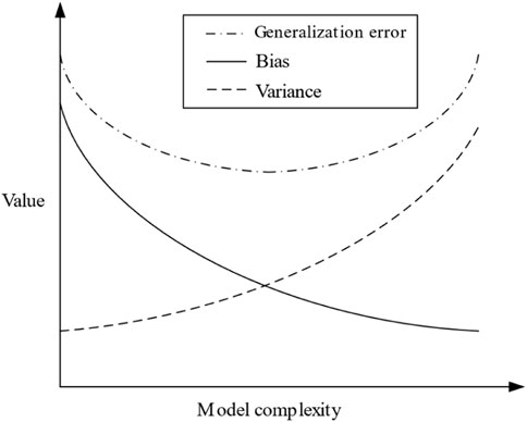
FIGURE 15. Bias and variance dilemma: the general relationship between bias and variance.

Zhou (2016) offers theoretical justification for ensemble algorithms that can improve the accuracy and stability of models and reduce generalization errors by enhancing the diversity of models. The conventional ensemble algorithms include bagging, boosting, and stacking based methods.

Bagging can reduce the variance of the ensemble model by sampling the dataset, training multiple regression models of the same type separately, and weighting the prediction results of the models to obtain the final output. Boosting uses the next model to predict the residuals of the previous model. Finally, it combines the prediction results of multiple weak regression models with an additive model, which can reduce the bias of the ensemble model.

Stacking has a two-layer structure, using different regression models to predict the dataset in the first layer and the prediction results as the dataset to train the meta-model in the second layer. Relearning the prediction results may obtain higher generalization performance.

This paper uses three ensemble algorithms to optimize the neural network, with the structure shown in Figure 16.

FIGURE 16

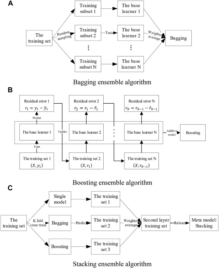
FIGURE 16. Concept schematic of three ensemble algorithm models. (A) Bagging ensemble algorithm, (B) Boosting ensemble algorithm, (C) Stacking ensemble algorithm.

4 Optimization and evaluation of artificial neural network model

The artificial neural network can model non-linear relationships between variables. Macroscopically, it partitions the data space by progressive decomposition and relies on the scale of the model to obtain better performance. The artificial neural network has a wide range of applications. However, the relationship between targets and features varies so much in datasets of different scenarios that it is difficult to use the comparative results on one dataset as a guide to another. This paper is more interested in how the ANN performs in the specific application scenario of the heat pipe cooled reactor’s start-up and power-up processes and how to comprehensively evaluate the neural network’s applicability.

Therefore, this section builds a peak power prediction model for the heat pipe cooled reactor’s start-up and power-up processes based on an artificial neural network, optimizes the model by adjusting the model structure, and evaluates the model’s performance in terms of cost, accuracy, interpretability, and uncertainty using a comprehensive framework.

4.1 Model optimization

The accuracy of neural network models is affected by numerous factors. The hyperparameters affect the prediction ability by determining the complexity of the model, the training data directly affect the effect of model learning, and the ensemble algorithms can achieve performance improvement through the combination of multiple models.

4.1.1 Hyperparameters optimization

The hyperparameters determine the complexity of the model. The learning ability of a simple model is limited, but as the complexity increases, the model overfits, i.e., gradually learns some properties of the training set and loses good generalization performance. Taking the power-up dataset as an example, the complexity of the model can be represented by hyperparameters that indicate the model structure size, such as the depth (n_dense) and width (n_hidden). The neural network will directly determine the size of the model. This section uses the training set to calculate the model parameters and the validation set to determine the degree of overfitting. Figure 17 shows the effect of hyperparameters on the overfitting of the neural network model.

FIGURE 17

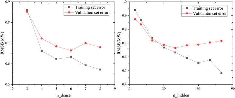
FIGURE 17. Influence of the neural network depth and width on overfitting.

The overfitting phenomenon can be observed in the training of the neural network. Although each neuron can use the complete samples, the increase in width due to the different weights still causes the effect of further division of the data space. The neural network that is too deep may cause parameters instability with vanishing gradient problems or exploding gradient problems due to the continued multiplication of multiple activation functions. Therefore, the hyper parameters should be tuned to alleviate the overfitting situation to get the prediction model with the best results.

This overfitting phenomenon of the model can be explained by the bias-variance dilemma, where the model complexity makes a difference in the effect of the bias and variance, thus leading to a change in the generalization error of the model, as shown in Figure 15. A model’s generalization error can always be decomposed into bias and variance, and the effect of hyperparameters on overfitting is a combination of the effects on bias and variance, respectively. The bias and variance are averaged over all possible datasets computed by the model and are only relevant to the model and not to the specific dataset.

In cases where datasets are difficult to obtain, the bias and variance of the model can be computed on the multiple datasets obtained by bootstrap replicates from the original dataset as shown in Figure 18 (Sofus et al., 2008).

FIGURE 18

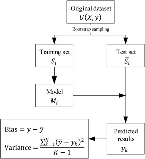
FIGURE 18. Flowchart of bias and variance calculation method.

Overfitting can be alleviated by adjusting the model hyperparameters and controlling the bias and variance in a suitable position. It is found that the bias of the neural network always decreases monotonically with the increase of depth or width. However, as the width increases, the variance is unimodal, and it is found that deeper models increase variance. Thus, the trend of the generalization error of the neural network with model complexity depends on the relative magnitude of bias and variance (Yang et al., 2020).

The artificial neural network is a low bias but high variance model and the generalization error depends mainly on the control of variance. For the neural network, the variance will increase if the model is too deep. The effect of width on variance is still unimodal, as shown in Figure 19, and performance can be further improved by widening.

FIGURE 19

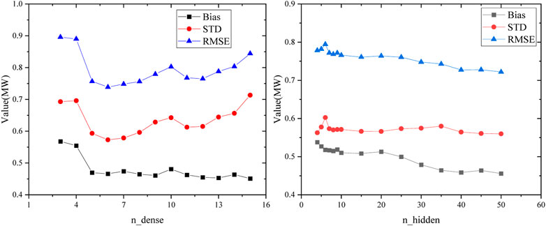
FIGURE 19. Influence of the neural network depth and width on bias and variance.

4.1.2 Dataset size

This section investigates the effect of dataset size on model error. Figures 20, 21 shows that the relationship between dataset size and model error has basically converged during the start-up and power-up processes, indicating that it is appropriate to use both datasets to train the neural network model. However, both datasets still have room for expansion to reduce the error. The neural network has many parameters. It is difficult for a small amount of data to learn more accurate parameters in the error back propagation process, so it is usually suitable for large datasets such as picture and text recognition.

FIGURE 20

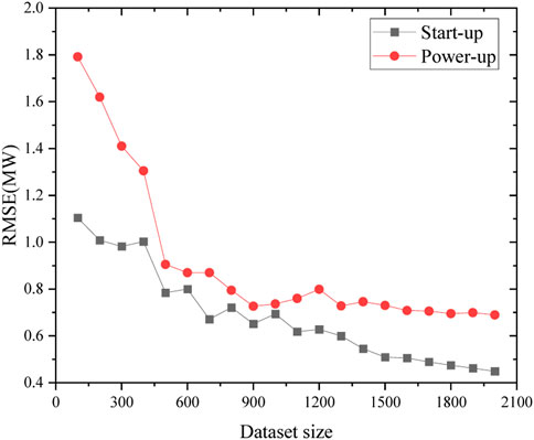
FIGURE 20. Influence of dataset capacity on RMSE in start-up and power-up processes.

FIGURE 21

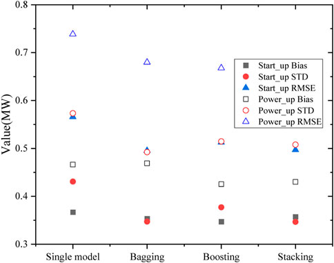
FIGURE 21. Effect of ensemble models in start-up and power-up processes.

4.1.3 Ensemble algorithms

Finally, the performance improvements of the three ensemble algorithms on the neural network model were compared. The results show that all three ensemble algorithms effectively reduce the generalization error of the models compared to single models.

The reduction effect on the variance and the bias is consistent with the theoretical analysis, with Bagging mainly reducing the variance and Boosting mainly reducing the bias. Considering that the neural network is a high variance but low bias model, the gains are more significant using Bagging than Boosting. While Stacking may obtain better results by relearning based on a simultaneous ensemble of a single model, Bagging and Boosting simultaneously.

5 Conclusion

The following research has been conducted in this paper. Firstly, the Monte Carlo sampling method and the deterministic model are combined to generate the heat pipe cooled reactor datasets in start-up and power-up processes. Then, the peak power prediction model based on the artificial neural network is established. Next, the influence of hyperparameters, dataset size, and ensemble algorithms on the model performance is studied. Finally, the following conclusions were obtained.

(1) The neural network model has a high prediction accuracy. The prediction error of the peak power in the heat pipe cooled reactor is 0.5658 MW for the start-up process and 0.7385 MW for the power-up process. It has a low uncertainty, and the predictive percentage errors of most samples are less than 20 percent.

(2) The neural network is a model with high variance and low bias. Thus, ensemble algorithms are mainly used to improve performance by reducing the variance of the model. The dataset size also impacts the model, and there is room for further expansion.

(3) The training and tuning costs of the neural network are high; the training time is 120 s on the start-up process dataset and 139 s on the power-up process dataset. But it has a relatively low prediction cost. The interpretability is weak too. It can be partially explained by passive interpretation, such as attribution interpretation and distance interpretation. It could be improved by combing neural networks and other algorithms in the future. Applying the neural network in scenarios that do not require high interpretability is more advantageous.

Data availability statement

The raw data supporting the conclusion of this article will be made available by the authors, without undue reservation.

Author contributions

YL: Methodology, software, writing—original draft. MH: Investigation, formal analysis. CP: Conceptualization, methodology, supervision. ZD: Software, Writing—original draft. ZW: Formal analysis.

Funding

The work described in this paper was supported by the Sichuan Province’s Outstanding Young Scientific and Technological Talent Project (2021JDJQ0034) and Science and Technology Innovation Team Program of Key Laboratory of NPIC (ZDSY-CXTD-21-04-001).

Conflict of interest

The authors declare that the research was conducted in the absence of any commercial or financial relationships that could be construed as a potential conflict of interest.

Publisher’s note

All claims expressed in this article are solely those of the authors and do not necessarily represent those of their affiliated organizations, or those of the publisher, the editors and the reviewers. Any product that may be evaluated in this article, or claim that may be made by its manufacturer, is not guaranteed or endorsed by the publisher.

Abbreviations

ANN, artificial neural network; BP, back propagation; CANDU, CANada Deuterium Uranium; CFX, Computational Fluid X; HPRTRAN, Heat Pipe cooled Reactor TRANsient analysis code; MCNP, Monte Carlo N Particle; M-P, McCulloch and Pitts; MSE, Mean Square Error; NBDT, Neural Backed Decision Tree; RMSE, Root Mean Square Error; SCWR FA, Super Critical Water Reactor Fuel Assembly; STD, standard deviation.

References

Bae, J., Kim, G., and Lee, S. J. (2021). Real-time prediction of nuclear power plant parameter trends following operator actions. Expert Syst. Appl. 186, 115848. doi:10.1016/j.eswa.2021.115848

CrossRef Full Text | Google Scholar

Dias, A. M., and Silva, F. C. (2016). Determination of the power density distribution in a PWR reactor based on neutron flux measurements at fixed reactor incore detectors. Ann. Nucl. Energy 90, 148–156. doi:10.1016/j.anucene.2015.12.002

CrossRef Full Text | Google Scholar

Geman, S., Bienenstock, E., and Doursat, R. (1992). Neural networks and the bias/variance dilemma. Neural Comput. 4, 1–58. doi:10.1162/neco.1992.4.1.1

CrossRef Full Text | Google Scholar

Gurgen, A. (2021). Development and assessment of physics-guided machine learning framework for prognosis system. Ann Arbor: North Carolina State University, 181.

Google Scholar

Hornik, K. (1991). Approximation capabilities of multilayer feedforward networks. Neural Netw. 4, 251–257. doi:10.1016/0893-6080(91)90009-t

CrossRef Full Text | Google Scholar

Ikonen, T. (2016). Comparison of global sensitivity analysis methods -Application to fuel behavior modeling. Nucl. Eng. Des. 297, 72–80. doi:10.1016/j.nucengdes.2015.11.025

CrossRef Full Text | Google Scholar

Ma, Y., Liu, J., Yu, H., Tian, C., Huang, S., Deng, J., et al. (2022). Coupled irradiation-thermal-mechanical analysis of the solid-state core in a heat pipe cooled reactor. Nucl. Eng. Technol. 54, 2094–2106. doi:10.1016/j.net.2022.01.002

CrossRef Full Text | Google Scholar

Ma, Y., Tian, C., Yu, H., Zhong, R., Zhang, Z., Huang, S., et al. (2021b). Transient heat pipe failure accident analysis of a megawatt heat pipe cooled reactor. Prog. Nucl. Energy 140, 103904. doi:10.1016/j.pnucene.2021.103904

CrossRef Full Text | Google Scholar

Ma, Y., Yang, X., and Liu, Y. (2021a). Reactivity feedback characteristic and reactor startup analysis of megawatt heat pipe cooled reactor[J]. Atomic Energy Sci. Technol. 50, 213–220. doi:10.7538/yzk.2021.zhuankan.0121

CrossRef Full Text | Google Scholar

Mcclure, P., Poston, D., and Rao, D. (2015). Design of megawatt power level heat pipe reactors[R]. Los Alamos: Los Alamos National Lab.

Google Scholar

Song, S. (2002). Heat balance test for determined reactor core power. Nucl. Power Eng. 23, 82–86. doi:10.3969/j.issn.0258-0926.2002.02.018

CrossRef Full Text | Google Scholar

Sterbentz, J. W., Werner, J. E., and Mckellar, M. G. (2017). Special purpose nuclear reactor (5MW) for reliable power at remote sites assessment report[R]. Idaho Falls. United States: Idaho National Lab.

Google Scholar

Wan, A., Dunlap, L., Ho, D., Jihan, Y., Lee, S., and Jin, H. (2020). NBDT:Neural-Based decision trees arXiv. arXiv (USA), 14.

Google Scholar

Xi, X., Xiao, Z. J., Yan, X., Li, Y. L., and Huang, Y. P. (2013). The axial power distribution validation of the SCWR fuel assembly with coupled neutronics-thermal hydraulics method. Nucl. Eng. Des. 258, 157–163. doi:10.1016/j.nucengdes.2013.01.031

CrossRef Full Text | Google Scholar

Zhang, X. Y., Trame, M. N., Lesko, L. J., and Schmidt, S. (2015). Sobol sensitivity analysis: A tool to guide the development and evaluation of systems pharmacology models. CPT pharmacometrics Syst. Pharmacol. 4, 69–79. doi:10.1002/psp4.6

PubMed Abstract | CrossRef Full Text | Google Scholar

Zhong, R., Ma, Y., and Deng, J. (2021). Reactor startup characteristics of heat pipe cooled reactorwith multiple FeedbackMechanism[J]. Nucl. Power Eng. S2, 104–108. doi:10.13832/j.jnpe.2021.S2.0104

CrossRef Full Text | Google Scholar

Zhou, Z. H. (2016). Machine learning. Beijing: Tsinghua University Press.

Google Scholar