Optimal Planning of Integrated Energy System Considering Convertibility Index

1 Introduction

Nowadays, developing an IES is considered an effective pattern to improve energy efficiency and reduce energy supply costs. IESs break the limitation of a single-energy system, which is the development trend of future energy systems (Mancarella, 2014; Fan et al., 2021). IESs contain various energy flow types in energy transmission and conversion systems, including electricity, heating water, cooling water, and natural gas. In conventional non-IESs, each type of energy system is operated independently. However, energy can be converted between various energy flow types in the IESs. For example, the energy carried by electricity, heating water, cooling water, and gas flows can be mutually converted in many devices such as CHP (combined heat and power), CCHP (combined cold, heat, and power supply), EHPs (electric heat pumps), and air conditioners (ACs) (Mancarella, 2014).

This study aims to solve the IES planning problem considering the flexibility requirement. Conversion availability between different energy flow types is a critical feature and advantage of the IES (Jiang et al., 2020), which increases the flexibility of the IES operation. For example, if a fault occurs in the gas transmission system, the gas consumer can have access to gas by power-to-gas (P2G) devices. Another example is that the consumer can alternatively select energy types according to real-time prices. It is worth noting that more energy conversion devices often indicate higher flexibility of the IES, although the cost will be higher, while less energy conversion devices might provide insufficient energy and result in high operation cost. Therefore, the planning problems of the IES are highly related to the flexibility of the IES, and there is a tradeoff between IES flexibility and the total cost.

1.1 Existing Methods About Assessment of IES Flexibility

In the area of power systems, flexibility assessment has been extensively studied. Generation adequacy metrics, such as loss of load expectation (LOLE), expected energy not served (EENS), loss of largest unit (LLU), and insufficient ramping resource expectation (IRRE), have been widely used in flexibility assessment of power systems (Lannoye et al., 2012). Nosair and Bouffard (2015) proposed the concept of a flexibility envelope to describe the flexibility potential dynamics of a power system and its individual resources in the operational planning time frame. For a power system with sustainable generation, Ma et al. (2013) presented an “offline” index to estimate the technical ability of both individual generators and the generation mix to provide the required flexibility. In the field of the IES, Clegg and Mancarella (2016) focused on the power system and the gas system and presented a methodology to quantify the flexibility of the gas network of the power system. Coelho et al. (2020) assessed the flexibility of multi-energy residential and commercial buildings. The authors of this study previously proposed a metric named “load replaceability” to assess the flexibility of the IES in the demand side (Zheng et al., 2019). Meanwhile, more assessment has been made from the perspective of energy efficiency, such as utilization efficiency (EUE) and exergy efficiency (EXE) (Su et al., 2021). Huang et al. (2021) presented indices for IES vulnerability assessment to find the key components for improving IES reliability. Moreover, several literature studies have been undertaken to improve the flexibility of the IES (for example, Good and Mancarella, 2019).

1.2 Existing Methods for Assessment of IES Planning

IES planning refers to making optimal plans for constructing an IES. In recent years, much work on IES planning has been carried out (Fan et al., 2021). Mendes et al. (2011), Mirakyan and De Guio (2013), Mirakyan and De Guio (2015), Farrokhifar et al. (2020) reviewed the research studies in the field of IES planning. Xiang et al. (2020) and Wang et al. (2022) studied the IES planning problem from economic aspects, in which the cost–benefit and exergy efficiencies are analyzed. The investment constraints in IES planning problems are included in Wang et al. (2019a). The environmental issues in IES planning problems are considered in Qin et al. (2019). The electricity–hydrogen IES planning problem is studied in Pan et al. (2020). To consider the participants in the market, a game-theoretic planning method is proposed for IESs (Zhang et al., 2019). Wang et al. (2021) proposed a planning method for the IES based on the life cycle. In Lei et al. (2020), a pipeline risk index for energy network expansion planning is defined as an IES planning problem. As for the mathematical models of IES planning, Ma et al. (2018) optimized the system structure and size of an IES and modeled the problem as a mixed integer linear programming (MILP) problem. Koltsaklis et al. (2014) presented a linear mixed integer programming model for optimal designing and operational planning of energy networks. Koltsaklis and Knápek (2021) presented an optimization framework for optimal scheduling of a multi-energy microgrid based on mixed integer programming techniques, consisting of a number of aggregated end users. In Nicolosi et al. (2021), a novel mixed integer linear programming (MILP) optimization algorithm was developed to compute the optimal management of a micro-energy grid. Zhou et al. (2013) provided a generic energy system engineering framework for optimal designing of IESs in China. Wang et al. (2022), Jing et al. (2018), Wang et al. (2019b), and Qin et al. (2019) built up the optimal planning problem of IESs as multi-objective optimization problems, and the evolutional algorithms were used to solve the problems. A hybrid algorithm combining tabu search algorithm and GA was used in Wang et al. (2022), and a hybrid algorithm combining differential evolution and particle swarm optimization was used in Jing et al. (2018). Wang et al. (2019b) presented a two-stage optimization method for a coupled capacity planning and operation problem, in which the first stage is to optimize the type and capacity of the IES by the non-dominated sorting genetic algorithm-II (NSGA-II) and the second stage is to solve the optimal dispatch and operation problem by MILP. Xiao et al. (2018) modeled IES planning as a bi-level problem in which the optimal operation of the IES under different probability scenarios is the lower-level problem and the optimal planning and design of the IES is the upper-level problem. Wang et al. (2019c) proposed an expansion planning model for the IES to minimize the total cost over the planning horizon and proposed a second-order cone programming and a modified piecewise linearization approach to convert the original mixed integer non-linear programming model to a mixed integer second-order cone programming model.

Based on the aforementioned review, the advantages of the existing models mainly include the following: 1) detailed models of different devices of the IES have been well explored and established; 2) many factors, such as the uncertainties and environmental factors, have been considered. The disadvantages of the existing models mainly include the following: 1) very less attention has been paid directly to the flexibility assessment of the IES, and the existing work on IES flexibility assessment is mainly focused on capacity adequacy. Therefore, there remains a gap in the literature regarding quantitative assessment of the conversion flexibility of the IES. 2) Although plenty of efforts have been focused on IES planning problems, the planning problem has not been fully considered with the flexibility indexes. As IES planning techniques evolve with the challenge of integrating energy conversion devices, the appropriate flexibility to manage different types of energy flows and energy conversions needs to be included.

In this work, we studied the flexibility assessment of the IES regarding the energy conversion process between different energy flow types and proposed a planning method for IESs with CI constraints. The proposed method will be useful to IES planners, investors, or owners who are interested in the following: how to assess IES flexibility? What is the appropriate degree of IES flexibility? How to keep the cost efficiency with appropriate conversion flexibility? The main contributions include the following: 1) an index for quantitative assessment of the conversion flexibility of the IES is proposed. Different from the existing indexes in Clegg and Mancarella (2016), Zheng et al. (2019), and Coelho et al. (2020), the proposed index places the emphasis on flexibility assessment regarding the energy conversion process between different energy flow types. 2) We built a bi-level optimal planning problem of the IES with CI constraints. Different from the existing bi-level planning problems of the IES in Wang et al. (2019b), Xiao et al. (2018), and Wang et al. (2019c), the CI constraints are included in the IES planning to emphasize the conversion flexibility of the IES. A new feature of considering CI is that the planner can obtain the most cost-saving IES plans and meet their CI requirement at the same time.

The remaining of the article is organized as follows: Section 2 presents the CI definition and calculation method; Section 3 presents the bi-level optimization model of IES planning with CI constraints; Section 4 conducts a case study to validate the proposed method; and Section 5 gives conclusions and discussions.

2 Convertibility Index of Integrated Energy System

IESs contain a variety of energy flow types in energy transmission and conversion systems, including electricity, heating water, cooling water, and natural gas. Different energy flows are coupled and connected by energy conversion devices. Figure 1 shows energy conversions between the conversion devices in an IES.

FIGURE 1

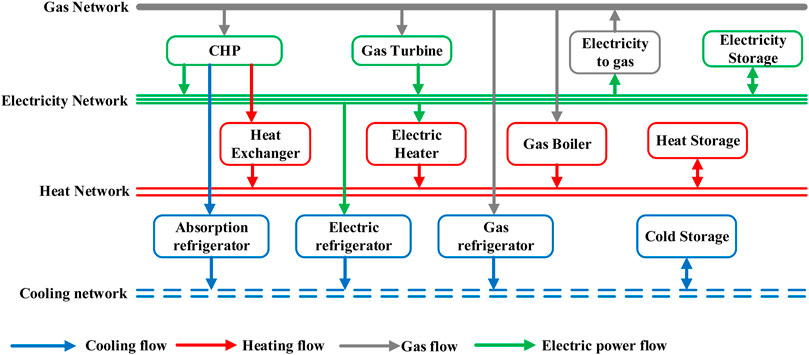
FIGURE 1. Energy conversions between conversion devices in the IES.

2.1 Definition of Convertibility

Compared to the traditional single-energy system, the IES provides extra availabilities in energy conversion. Here, we define such conversion availability as convertibility. For example, if an energy flow type, for example, A, can be converted from other types of energy flows, we say that energy flow A has convertibility. From the perspective of the end-users, if energy flow A can be converted from other energy flows, it means that energy flow A can be obtained from other types of energy flow and has convertibility. In Figure 1, the heat energy in the heat water pipeline can be converted from the energy in gas by the CHP and a heat exchanger; thus, the heat energy in this system has convertibility.

2.2 Definition of Convertibility Index of a Given Energy Flow Type

If we want to quantitatively assess convertibility, we need an index to measure it. Here, we define the CI of an energy flow type to reflect the conversion flexibility of this energy flow type. As for an IES, there exist four possible types of energy flows in the system. Denote the CI of the cooling flow, heating flow, electric power flow, and gas flow by ${\alpha }_C$, ${\alpha }_H$ , ${\alpha }_E$, and ${\alpha }_G$, respectively. The four CIs can be calculated by Eqs 1–4:

${\alpha }_c=\frac{1}{C_{\max }}{\displaystyle \sum _{i=1}^{M_C}{C}_i},(1)$

${\alpha }_H=\frac{1}{H_{\max }}{\displaystyle \sum _{i=1}^{M_H}{H}_i},(2)$

${\alpha }_E=\frac{1}{P_{\max }}{\displaystyle \sum _{i=1}^{M_E}{P}_i},(3)$

${\alpha }_G=\frac{1}{G_{\max }}{\displaystyle \sum _{i=1}^{M_G}{G}_i},(4)$

where ${\alpha }_C$, ${\alpha }_H$, ${\alpha }_E$, and ${\alpha }_G$ represent the CI of the cooling flow, heating flow, electric power flow, and gas flow, respectively; $C_i$ represents the rated power of the No. i device which can convert energy from heat, power, or gas flow into cooling flow; $C_{\max }$ represents the maximum cooling power of the cooling network; $H_i$ represents the rated power of the No. i device which can convert energy from cooling, power, or gas flow into heating flow; $H_{\max }$ represents the maximum heating power of the heating network; $P_i$ represents the rated power of the No. i device which can convert energy from heat, cooling, or gas flow into electric power; $P_{\max }$ represents the maximum power supply of the power grid; $G_i$ represents the rated power of the No. i device which can convert energy from heat, power, or cooling flow into gas; and $G_{\max }$ represents the maximum power supply of the gas network.

With the abovementioned definition, the CI of a given energy flow type can reflect the conversion capabilities between the given energy flow and the other energy flow types. If energy can be obtained from larger capacities of the energy conversion devices, the CI of the given energy flow type will be higher. When the CI of a given energy flow is larger than 1, it means that the energy it needs can be fully converted from other energy flow types.

2.3 Definition of Convertibility Index of an Integrated Energy System (α_IES)

${\alpha }_{IES}$ reflects the overall conversion flexibility of the IES, which is basically based on the CIs of different energy flows. The CI of the IES is defined by taking the weighted average of the CIs ∗ conversion path factor ∗ maximum power of the network, as shown in Eq. 5. In this definition, we introduce a new parameter, “conversion path factors” (k), to describe the flexibility of energy conversion paths. For example, two energy flow types, for example, heating and electricity, have the same CI, that is, ${\alpha }_H$ = ${\alpha }_E$. However, the energy in heating can be converted from only one type of other energy flow, while the energy in electricity can be converted from three types of other energy flows. Obviously, the electricity system with three “energy conversion paths” is more robust. In such a case, we can set $k_E$ to be larger than $k_G$. Note that it is an objective setting, which can be determined by the system operators or planners. When ${\alpha }_{IES}$ is larger than 1, it means that the weighted average CIs of different energy flow types are larger than 1, indicating that the energy consumption by the IES on average can be fully converted from other energy flow types rather than depending on its original energy flow type.

${\alpha }_{IES}=\frac{k_C{\alpha }_E{C}_{\max }+k_H{\alpha }_E{H}_{\max }+k_E{\alpha }_E{P}_{\max }+k_G{\alpha }_G{G}_{\max }}{C_{\max }+H_{\max }+P_{\max }+G_{\max }},(5)$

where ${\alpha }_{IES}$ represents the CI of the IES; ${\alpha }_C$, ${\alpha }_H$, ${\alpha }_E$, and ${\alpha }_G$ represent the CIs of the cooling flow, heating flow, electric power flow, and gas flow, respectively; and $C_{\max }$, $H_{\max }$, $P_{\max }$, and $G_{\max }$ represent the maximum cooling, heating, power, and gas power of the cooling, heating, power, and gas network, respectively. $k_C$, $k_H$, $k_E$, and $k_G$ represent the conversion path factors, respectively. The energy flow types which have more conversion paths will be with higher conversion path factors.

3 Bi-Level Optimization Model of Integrated Energy System Planning Considering Convertibility Index

3.1 Framework

The optimal planning problem aims to minimize the total cost of the IES, and we built up a bi-level optimization problem to achieve the aim. Bi-level optimization is a special kind of optimization where one problem is embedded within another. The outer optimization task is commonly referred to as the upper-level optimization task, and the inner optimization task is commonly referred to as the lower-level optimization task. These problems involve two kinds of variables, referred to as the upper-level variables and the lower-level variables.

The bi-level problem of the IES planning is shown in Figure 2. The upper level of the model determines the types and numbers of the devices in the IES, and these decisions are the inputs of the lower-level model. As for the objective functions, the objective function of the upper-level model is to minimize the annual investment cost and the operation costs, while the objective function of the lower-level model is to minimize the operation cost with a given planned IES.

FIGURE 2

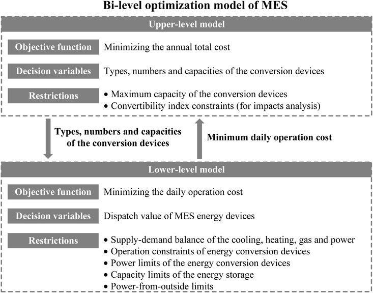
FIGURE 2. Bi-level optimization model of the IES.

3.2 Upper-Level Planning Model

The upper-level planning model takes the minimum annual total cost of the system as the objective function. The annual total cost mainly includes the investment cost of the devices and the yearly system operation cost. The decision variables are the types and numbers of the IES devices. The constraints include the system maximum capacity constraints. For studying the impacts of the CI, the constraints with the CI are also included.

3.3 Lower-Level Planning Model

The lower-level planning model takes the minimum operation cost in the typical day as the objective function. The decision variables are the dispatch values of the conversion devices determined by the upper-level problem. The constraints include the supply–demand balance constraints of the cooling, heating, gas, and power; the operation constraints of energy conversion devices; the power limits of the energy conversion devices; the capacity limits of the energy storage; and the power-from-outside limits.

Note that some assumptions have been made for this problem (Mancarella, 2014; Zheng et al., 2019). 1) All the parameters needed for the optimization are assumed to be known. 2) The changes in the parameters along with the operation status are neglected to simplify the model. For example, the temperature impacts on the efficiencies are not considered. Considering that the planning problem covers a long time period, the changes in the parameters are marginal, and therefore the changes in the parameters are neglected. 3) The energy flow optimization is not included. Since the studied IES is not a huge system with long-distance transmission, the energy transmission limits can be neglected. 4) The storage within the gas, cold, and hot water pipes is not considered. For an IES without long-distance transmission, the amount of gas and water within the pipes is minor. Thus, the storage within the pipes is neglected.

3.4 Upper-Level Model

The objective function of the upper-level problem is to minimize the annual total cost, as shown by Eq. 6. The annual total cost includes the annual investment cost of the devices and the yearly system operation cost in the whole year. Here, the investment cost is represented by the annual investment cost ($F_{INV}$). The yearly system operation cost is the sum of the daily operation cost. To make the calculation of the operation cost simpler, we selected several days as the typical day scenarios instead of optimizing every operation day in the model. With typical day scenarios, only the operations with the selected days are optimized, which largely decreases the computation burden of the lower-level model. The number of the days of each typical day scenario ($D_s$) will be the weight coefficients in the objective function.

$\min F=F_{INV}+{\displaystyle \sum _{s=1}^S{D}_s}{F}_{OP,s},(6)$

where $F_{INV}$ is the annual investment cost, $s$ is the index of the typical day scenario, $S$ is the total number of the typical day scenarios, $D_s$ is the number of days of the typical day scenario $s$, and $F_{OP,s}$ is the operation cost of the typical day scenario $s$.

The annual investment cost ($F_{INV}$) is the average value of the total investment of devices purchased at the beginning of the year. The calculation of the annual investment cost and the capital recovery factor are given as follows (Eqs 7, 8):

$F_{INV}={\displaystyle \sum _{i=1}^I{n}_i{C}_i{M}_i{\delta }_i}\mu (r,Y_i),(7)$

$\mu (r,Y_i)=\frac{r{(r+1)}^{Y_i}}{{(r+1)}^{Y_i}-1},(8)$

where $i$ is the index of all the types of IES devices; $I$ is the total type number of all the IES devices; $n_i$ is the installed number of the device of type $i$; $C_i$ is the rated capacity of the device of type $i$; $M_i$ is the investment cost per unit capacity of device $i$; ${\delta }_i$ is a binary variable which indicates whether the device $i$ is selected, where ${\delta }_i=1$ means it is selected, otherwise ${\delta }_i=0$; $\mu (r,Y_i)$ is the capital recovery factor; $Y_i$ is the technical lifetime of device $i$; and $r$ is the annual interest rate of the capital.

The constraints include maximum capacity constraints. To study the impacts of the CI, the constraints with the CI are also included.

3.4 1 Maximum Capacity Constraints

The capacities of each type of the devices should not be larger than a given value. For a given type which might be with more than one device, the total capacities of the given type should not be larger than a given value, as shown by Eq. 9

$0\le n_i\cdot C_i\le C_i^{\max },(9)$

where $n_i$is the installed number of the device of type $i$, $C_i$ is the rated capacity of the device of type $i$, and $C_i^{\max }$ is the maximum capacity limit of the device of type $i$.

3.4 2 Convertibility Index Constraints

The main difference of the proposed IES planning model from the previous research is that the CI constraints are included. The CI can be calculated by Eq. 10 in which some variables are decision variables of the upper-level model. In the upper-level model, the CI of the IES is fixed at a given value ${\alpha }_{\text{0}}$, as shown by Eq. 11. The ${\alpha }_{\text{0}}$ can be determined based on the experience and flexibility requirement of the IES planner. For the IES planners, they can at first optimize the problem without setting the CI constraint to obtain the benchmark of CI and cost for the IES. After that, the planners can make the decisions on their own whether the current CI and cost are acceptable or not. If the planners want to set a specific requirement for CI, they can add the CI constraints.

${\alpha }_{IES}=\frac{k_C{\alpha }_C{C}_{\max }+k_H{\alpha }_H{H}_{\max }+k_E{\alpha }_E{P}_{\max }+k_G{\alpha }_G{G}_{\max }}{C_{\max }+H_{\max }+P_{\max }+G_{\max }},(10)$

${\alpha }_{IES}={\alpha }_{\text{0}},(11)$

where ${\alpha }_{IES}$ represents the CI of the IES and ${\alpha }_{\text{0}}$ represents the given value of the CI of the IES.

3.5 Lower-Level Model

The objective function of the lower-level problem is to minimize the daily operation cost. The daily operation cost consists of four parts, as shown by (Eq. 12): the energy cost (Eq. 13), the maintenance cost (Eq. 14), the degradation cost of the energy storage (Eq. 15), and the carbon emission cost (Eq. 16). For simplification, the subscript “s” representing the scenarios is neglected in the lower-level model.

$F_{OP}=F_E+F_M+F_D+F_{CO2},(12)$

where $F_{OP}$ is the operation cost, $F_E$ is the energy cost, $F_M$ is the maintenance cost, $F_D$ is the degradation cost of the energy storage, and $F_{CO2}$ is the carbon emission cost.

$F_E={\displaystyle \sum _{t=1}^T[{\lambda }_{grid}\left(t\right)P_{grid}\left(t\right)+{\lambda }_{gas}\left(t\right)\frac{G\left(t\right)}{R_{gas}}+{\lambda }_{hot}\left(t\right)P_{hot}\left(t\right)+{\lambda }_{cold}\left(t\right)P_{cold}\left(t\right)]\text{Δ}t},(13)$

$F_M={\displaystyle \sum _{t=1}^T{\displaystyle \sum _{i=1}^I{\lambda }_i{P}_i^{out}\left(t\right)\text{Δ}t}},(14)$

$F_D={\displaystyle \sum _{t=1}^T\left[{\lambda }_{PS}{P}_{PS}^S\left(t\right)+{\lambda }_{HS}{H}_{HS}^S\left(t\right)+{\lambda }_{CS}{C}_{CS}^S\left(t\right)\right]\text{Δ}t},(15)$

$F_{CO2}={\displaystyle \sum _{t=1}^T{\lambda }_{CO2}\left[{\lambda }_{grid}{P}_{grid}\left(t\right)+{\lambda }_{gas}{G}_{grid}\left(t\right)+{\lambda }_{hot}{P}_{hot}\left(t\right)+{\lambda }_{cold}{P}_{cold}\left(t\right)\right]\text{Δ}t},(16)$

where $t$ represents the dispatch interval; $T$ represents the total number of dispatch intervals; ${\lambda }_{grid}\left(t\right)$ and $P_{grid}\left(t\right)$ represent electricity price and electricity purchase power at time $t$, respectively; ${\lambda }_{gas}\left(t\right)$ and $G\left(t\right)$ represent gas price and gas purchase power at time $t$, respectively; $R_{gas}=9.77(kw\cdot h/m^3)$ represents the calorific value of gas; ${\lambda }_{hot}\left(t\right)$ and $P_{hot}\left(t\right)$ represent heating price and heating energy purchase power at time $t$, respectively; ${\lambda }_{cold}\left(t\right)$ and $P_{cold}\left(t\right)$ represent cooling price and cooling energy purchase power at time $t$, respectively; ${\lambda }_i$ represents the maintenance cost of unit power of No. i device; $P_i^{out}\left(t\right)$ represents output power of No. i device at time $t$; ${\lambda }_{PS}$, ${\lambda }_{HS}$, and ${\lambda }_{CS}$ represent the degradation rate per unit quantity of power, heating energy, and cooling energy, respectively; $P_{PS}^S\left(t\right)$, $H_{HS}^S\left(t\right)$, and $C_{CS}^S\left(t\right)$ represent the electricity, heating energy, and cooling energy stored at time t, respectively; ${\lambda }_{grid}$, ${\lambda }_{gas}$, ${\lambda }_{hot}$, and ${\lambda }_{cold}$ represent the emission coefficient of the electricity, and gas, heating, and cooling energy, respectively; and ${\lambda }_{CO2}$ represents carbon emission tax prices.

The constraints include the following: the supply–demand balance constraints of the cooling, heating, gas, and power; the operation constraints of energy conversion devices; the power limits of the energy conversion devices; the capacity limits of the energy storage; and the power-from-outside limits.

3.5.1 Supply–Demand Balance Constraints

Similar to the power balance equation in electric grids, the energy supply and demand balances of each energy flow type need to be constrained in the IES. Note that the energy supply side of the type A energy flow might contain the energy flow to be converted to type A, and the energy flow to be converted to other types. Moreover, the energy in and out of the energy storage is also considered. Finally, the supply–demand balance constraints of cooling energy (Eq. 17), heating energy (Eq. 18), electric power energy (Eq. 19), and gas energy (Eq. 20) are guaranteed.

${\displaystyle \sum _{i=1}^{M_C}{P}_{C,i}\left(t\right)}+{\displaystyle \sum _{i=1}^{N_C}[P_{CS,i}^R\left(t\right)-P_{CS,i}^S\left(t\right)]}+P_{cold}^{dir}\left(t\right)={\displaystyle \sum _{i=1}^{L_C}{P}_{cold,i}^{load}\left(t\right)},(17)$

${\displaystyle \sum _{i=1}^{M_H}{P}_{H,i}\left(t\right)}+{\displaystyle \sum _{i=1}^{N_H}[P_{HS,i}^R\left(t\right)-P_{HS,i}^S\left(t\right)]}+P_{hot}^{dir}\left(t\right)={\displaystyle \sum _{i=1}^{L_H}{P}_{hot,i}^{load}\left(t\right)},(18)$

${\displaystyle \sum _{i=1}^{M_P}{P}_{P,i}\left(t\right)}+{\displaystyle \sum _{i=1}^{N_P}[P_{PS,i}^R\left(t\right)-P_{PS,i}^S\left(t\right)]}+P_{grid}^{dir}\left(t\right)={\displaystyle \sum _{i=1}^{L_P}{P}_{grid,i}^{load}\left(t\right)},(19)$

${\displaystyle \sum _{i=1}^{M_G}{P}_{G,i}\left(t\right)}+{\displaystyle \sum _{i=1}^{N_G}[P_{GS,i}^R\left(t\right)-P_{GS,i}^S\left(t\right)]}+P_{gas}^{dir}\left(t\right)={\displaystyle \sum _{i=1}^{L_G}{P}_{gas,i}^{load}\left(t\right)},(20)$

where $t$ has the same meaning as in Eq. 14; $P_{C,i}\left(t\right)$, $P_{H,i}\left(t\right)$, $P_{P,i}\left(t\right)$, and $P_{G,i}\left(t\right)$ represent the output power of the No. i energy conversion device converted into cooling, heating, electricity, and gas power at time $t$, respectively; $M_C$, $M_H$, $M_P$, and $M_G$ represent the number of energy conversion devices converted into cooling, heating, electricity, and gas flow, respectively; $P_{CS,i}^R\left(t\right)$, $P_{HS,i}^R\left(t\right)$, $P_{PS,i}^R\left(t\right)$, and $P_{GS,i}^R\left(t\right)$ represent cooling, heating, electricity, and gas power released by the No. i storage devices of cooling, heating, electricity, and gas energy at time $t$, respectively; $P_{CS,i}^S\left(t\right)$, $P_{HS,i}^S\left(t\right)$, $P_{PS,i}^S\left(t\right)$, and $P_{GS,i}^S\left(t\right)$ represent cooling, heat, electricity, and gas energy stored by the No. i cooling, heat, electric, and gas energy storage system at time $t$, respectively; $N_C$, $N_H$, $N_P$, and $N_G$ represent the number of cooling, heating, electricity, and gas energy storage system, respectively; $P_{cold}^{dir}\left(t\right)$, $P_{hot}^{dir}\left(t\right)$, $P_{grid}^{dir}\left(t\right)$, and $P_{gas}^{dir}\left(t\right)$ represent the cooling, heating, electricity, and gas energy power directly provided by the system at time $t$, respectively; $P_{cold,i}^{load}\left(t\right)$, $P_{hot,i}^{load}\left(t\right)$, $P_{grid,i}^{load}\left(t\right)$, and $P_{gas,i}^{load}\left(t\right)$ represent load power of the No. i cooling, heating, electricity, and gas at time $t$, respectively; and $L_C$, $L_H$, $L_P$, and $L_G$ represent the number of cooling, heating, electricity, and gas load, respectively.

3.5.2 Operation Constraints of Energy Conversion Devices: Combined Heat and Power

The CHP plant generates electricity and heat simultaneously. The relationships between input gas power and output electricity or heat power of the backpressure CHP plant are given by Eq. 21 and Eq. 22. The surplus heat, generated by the CHP plant, is partly converted to cooling energy by an absorption refrigerator and partially converted to heating energy by a heat exchanger. The output cooling power of the absorption refrigerator and the output heating power of the heat exchanger are given by Eq. 23 and Eq. 24:

$P_{CHP}\left(t\right)={\eta }_P{G}_{CHP}\left(t\right),(21)$

$Q_{CHP}\left(t\right)=c_{QP}{P}_{CHP}\left(t\right),(22)$

where ${\eta }_{CHP}$ represents the power generation efficiency of the CHP; $c_{QP}$ represents the ratio of electricity-to-heat, which is a constant in this model; $Q_{CHP}\left(t\right)$ represents the surplus heat power of the CHP plant; and $G_{CHP}\left(t\right)$ and $P_{CHP}\left(t\right)$ represent the input gas power and output electricity power of the CHP plant, respectively.

$C_{AC}\left(t\right)={\eta }_{AC}\left(1-{\gamma }_{HC}\right)Q_{CHP}\left(t\right),(23)$

$H_{HX}\left(t\right)={\eta }_{HX}{\gamma }_{HC}{Q}_{CHP}\left(t\right),(24)$

where ${\eta }_{AC}$ and ${\eta }_{HX}$ represent the energy efficiency ratio of the absorption refrigerator and heat exchanger, respectively; ${\gamma }_{HC}$ represents the proportion ratio of the heat exchanger; $C_{AC}\left(t\right)$ represents the output cooling power of the absorption refrigerator; and $H_{HX}\left(t\right)$ represents the output heating power of the heat exchanger.

3.5.3 Operation Constraints of Energy Conversion Devices: Gas Turbine

A gas turbine converts gas energy into electricity energy. The relationship between unit output and gas input per unit time is as follows (Eq. 25):

$P_{GT}\left(t\right)={\eta }_{GT}{G}_{GT}\left(t\right),(25)$

where ${\eta }_{GT}$ represents the energy efficiency ratio of the gas turbine and $G_{GT}\left(t\right)$ and $P_{GT}\left(t\right)$ represent the input gas power and output electricity power of the gas turbine, respectively.

3.5.4 Operation Constraints of Energy Conversion Devices: Gas Boiler

A gas boiler converts gas energy into heat energy. The relationship between output heat power and gas input per unit time is as follows (Eq. 26):

$H_{GB}\left(t\right)={\eta }_{GB}{G}_{GB}\left(t\right),(26)$

where ${\eta }_{GB}$ represents the energy efficiency ratio of the gas boiler and $G_{GB}\left(t\right)$ and $H_{GB}\left(t\right)$ represent the input gas power and output heat power of the gas boiler, respectively.

3.5.5 Operation Constraints of Energy Conversion Devices: Electric Refrigerator and Electric Heater

An electric refrigerator and electric heater convert electricity power to cooling power and heat power, respectively. The relationships between output power and input power are given by Eq. 27 and Eq. 28:

$C_{PC}\left(t\right)={\eta }_{PC}{P}_{PC}\left(t\right),(27)$

$H_{PH}\left(t\right)={\eta }_{PH}{P}_{PH}\left(t\right),(28)$

where ${\eta }_{PC}$ and ${\eta }_{PH}$ represent the energy efficiency ratio of the electric refrigerator and electric heater, respectively; $P_{PC}\left(t\right)$ and $C_{PC}\left(t\right)$ represent the input electricity power and output cooling power of the electric refrigerator, respectively; and $P_{PH}\left(t\right)$ and $H_{PH}\left(t\right)$ represent the input electricity power and output heat power of the electric heater, respectively.

3.5.6 Power Limits of Energy Conversion Devices

The output of the conversion system has its lower/upper limit. The lower/upper output power limits of all kinds of energy conversion devices are given as (Eqs 29–32)

$P_{-C,i}\le P_{C,i}\left(t\right)\le {\overline{P}}_{C,i},(29)$

$P_{-H,i}\le P_{H,i}\left(t\right)\le {\overline{P}}_{H,i},(30)$

$P_{-P,i}\le P_{P,i}\left(t\right)\le {\overline{P}}_{P,i},(31)$

$P_{-G,i}\le P_{G,i}\left(t\right)\le {\overline{P}}_{G,i},(32)$

where $P_{C,i}$, $P_{H,i}$, $P_{P,i}$, and $P_{G,i}$ represent the lower limit of the output power of cooling, heat, electric, and gas energy of the No. i energy conversion device, respectively; and ${\overline{P}}_{C,i}$, ${\overline{P}}_{H,i}$, ${\overline{P}}_{P,i}$, and ${\overline{P}}_{G,i}$ represent the upper limit of the output power of cooling, heat, electric, and gas energy of the No. i energy conversion device, respectively.

3.5.7 Operation Constraints of Energy Storage Devices

The operation constraints of cooling storage, heating storage, and power storage devices mainly include the energy storage state constraints of each device, the energy balance constraints of the energy storage and discharge process, and the energy storage and discharge power constraints. Taking the power energy storage as an example, the operation constraints are given as follows (Eqs 33–39):

$S_{PS}\left(t\right)=(1-{\eta }_{PS})S_{PS}(t-1)+{\eta }_{PS}^S{P}_{PS}^S\left(t\right)-P_{PS}^R\left(t\right)/{\eta }_{PS}^R,(33)$

$S_{PS}^{\min }\le S_{PS}\left(t\right)\le S_{PS}^{m\text{ax}},(34)$

$S_{PS}\left(t_1\right)=S_{PS}\left(t_{end}\right),(35)$

$U_{PS}^S\left(t\right)P_{PS}^{\min }\le P_{PS}^{\text{S}}\left(t\right)\le U_{PS}^{\text{S}}\left(t\right)P_{PS}^{m\text{ax}},(36)$

$U_{PS}^R\left(t\right)P_{PS}^{\min }\le P_{PS}^R\left(t\right)\le U_{PS}^R\left(t\right)P_{PS}^{m\text{ax}},(37)$

$U_{PS}^R\left(t\right)+U_{PS}^R\left(t\right)\le 1,(38)$

$U_{PS}^R\left(t\right)\in \left(\mathrm{0,1}\right)U_{PS}^R\left(t\right)\in \left(\mathrm{0,1}\right),(39)$

where $S_{PS}\left(t\right)$ represents the state of charge in the electricity energy storage system at time $t$; $S_{PS}^{\min }$ and $S_{PS}^{\max }$ represent the minimal and maximal states of charge, respectively; $S_{PS}\left(t_1\right)$ represents the initial state of charge at the beginning of one operation cycle period; and $S_{PS}\left(t_{end}\right)$ represents the final state of charge at the end of one operation cycle period. When considering the periodicity of the operation of the ESS (energy storage system), the final state of charge of the previous operation cycle period should be equal to the initial state of charge of the next cycle. $U_{PS}^S$ and $U_{PS}^R$ are auxiliary variables (0–1 variable); $U_{PS}^S$ represents the on/off charge state; $U_{PS}^R$ represents the on/off discharge state; and $P_{PS}^{\min }$ and $P_{PS}^{\max }$ represent the minimum and maximum charge and discharge power of the energy storage system, respectively.

3.5.8 Power-From-Outside Limits

The lower/upper limits of purchase power of electricity, gas, cooling, and heating energy from the outside system are given as (Eqs 40–43)

$0\le P_{grid}\left(t\right)\le P_{grid}^{\max },(40)$

$0\le P_{gas}\left(t\right)\le P_{gas}^{\max },(41)$

$0\le P_{cold}\left(t\right)\le P_{cold}^{\max },(42)$

$0\le P_{hot}\left(t\right)\le P_{hot}^{\max },(43)$

where $P_{grid}^{\max }$, $P_{gas}^{\max }$, $P_{cold}^{\max }$, and $P_{hot}^{\max }$ represent the maximum limit of the IES to purchase electricity, gas, cooling, and heating energy from the outside system, respectively.

3.6 Solving algorithm

The proposed model is a bi-level problem. In this study, a hybrid GA–MILP algorithm (Shu et al., 2019) is selected to solve it. That is, GA (Grefenstette, 1988) is implemented in MATLAB to solve the upper-level problem for deriving optimal types and numbers of the devices in the IES. The lower-level problem which seeks for the optimal scheduling of IES and production tasks is an MILP problem, and it is solved by a commercial MILP solver in GAMS with ILOG/CPLEX (ILOG CPLEX, 2018). The connection between GAMS and MATLAB, which iteratively exchanges information between the upper-level and lower-level models, is realized by module GDXMRW. The detailed calculation procedure is presented in Figure 3, and the abstract pseudocode is shown in Table 1.

FIGURE 3

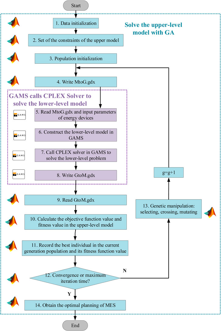
FIGURE 3. Hybrid GCA–MILP algorithm flowchart.

TABLE 1

TABLE 1. Abstract pseudocode of the hybrid GA–MILP solving algorithm.

It is worth mentioning that following three detailed settlements need to be made when applying the proposed model.

3.6.1 Penalty Function for Convertibility Index Constraint

In order to deal with the CI constraint, the penalty function is introduced into the model. The penalty function in GA is formulated as follows (Eq. 44):

$penalty=\{\begin{array}{c}0,if{\alpha }_{IES}-\zeta \le {\alpha }_{IES}\le {\alpha }_{IES}+\zeta ,\\ bigM,if{\alpha }_{IES}<{\alpha }_{IES}-\zeta or{\alpha }_{IES}>{\alpha }_{IES}+\zeta ,\end{array}(44)$

where $bigM$ is a large constant, which should be set much larger than the value of the objective function. For setting an appropriate big M, we suggest conducting the simulation without the CI constraint at first. Then the value of the objective function without the penalty function can be obtained. After that, the big M can be set as a big enough number; for example, 100 times higher than the value of the objective function. ${\alpha }_{IES}$is the optimized CI in the upper-level model and $\zeta$ is a small allowed deviation.

3.6.2 Fitness Function

In this study, the fitness function of GA is developed by using the ranking method, which is an off-the-shelf function provided by MATLAB. The principle of the ranking method is as follows: 1) sort the objective function of the individual and get the value of position of each individual. 2) According to the value of $Position$, calculate the fitness value of each individual as (Eq. 45)

$\text{itness}\left(Position\right)=2-2\times \frac{Position-1}{Nind-1},(45)$

where $Position$ represents the value arrangements and $Nind$ is the number of individuals in the population.

3.6.3 Termination Criterion

Considering that GA usually only ensures the local optimum, the termination criterion of this problem is set as one of the following two conditions: the optimal fitness value stays within a given threshold or the computation time has reached the maximum iteration time.

4 Case Study

This section presents a case study to verify the effectiveness of the proposed model. Section 4.1 provides the case data and settings. Section 4.2 presents the results without CI constraint. Section 4.3 studies the results with different CI constraints.

4.1 Case Settings and Data

In this section, we present a virtual case to validate the proposed method. This case includes 14 types of candidate energy conversion devices as shown in Figure 4. Some parameters are set according to Wenxia et al. (2020), Zhou et al. (2020), and Jie et al. (2021) and show the energy flow of the IES with all candidate devices. Table 2 presents the parameters of the IES, including capacities of energy conversion devices and energy storage devices, investment cost and maintenance cost per unit, conversion efficiencies, and service life. Three types of energy storage devices are set as must kept devices. Partial data and code are available online.¹

TABLE 2

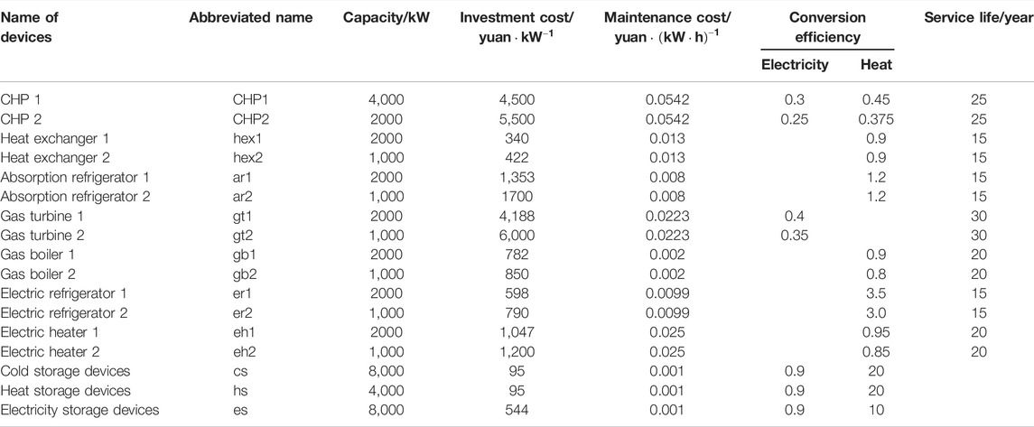
TABLE 2. Economic parameters of IES devices.

FIGURE 4

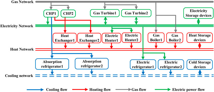
FIGURE 4. Energy conversions between the conversion devices of the case study.

4.1.1 Electricity Prices and Gas Prices

In China, electricity prices and gas prices for end users are mostly regulated and set by the provincial National Development and Reform Commission. In this study, we used “time-of-use” price data. The prices of peak, valley, and flat hours are given in Table 3. Note that the time periods of the peak–valley–flat of different places could be different. When using the proposed method, the users can set the prices based on the realized prices in their locations.

TABLE 3

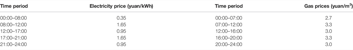
TABLE 3. “Peak–valley–flat” electricity and gas prices.

4.1.2 Heating and Cooling Prices

The heating prices are 0.225 yuan/kWh and the cooling prices are 0.65 yuan/kWh.

4.1.3 Carbon Emission Tax Prices

The carbon emission tax price is set at 0.14 yuan/kg. The emission efficiency of the IES system is set as 0.25 kg/kWh for electricity, 1.85 kg/m³ for gas, and 0 for cooling and heating.

4.1.4 Load Data

Load curves of three typical days, representing winter, summer, and spring/autumn days, respectively, are selected for the case study. The load curves of the three typical days are shown in Figures 5–7. The number of the three typical days is set as the same. The unit of the y-axis is the load ratio. The real load power is the product of the load ratio and the maximum load. The maximum loads are 7,000 kW for cooling, 8,000 kW for heating, 15,000 kW for power, and 10,000 kW for gas. For example, if the cooling power ratio is 0.9 for a given hour, the actual cooling power is 0.9 * 7,000 kW = 6,300 kW.

FIGURE 5

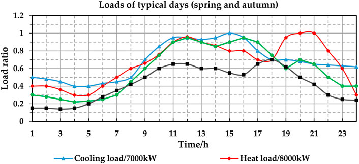
FIGURE 5. Representative daily load curve in spring and autumn.

FIGURE 6

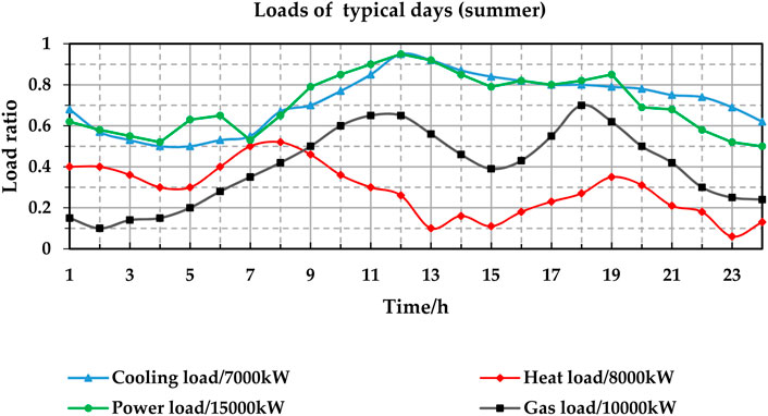
FIGURE 6. Representative daily load curve in summer.

FIGURE 7

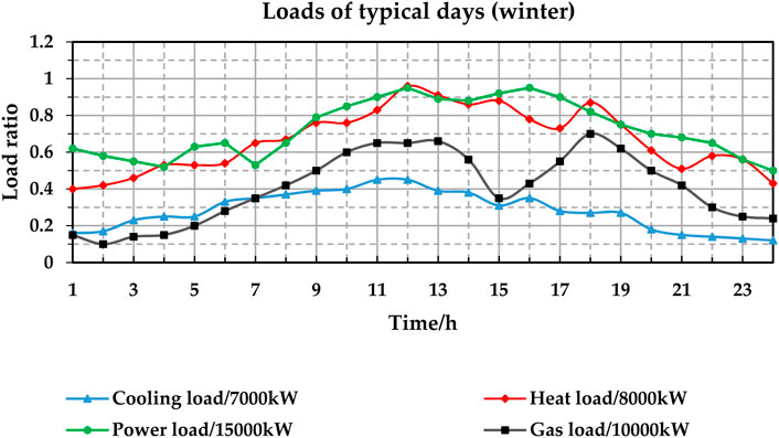
FIGURE 7. Representative daily load curve in winter.

The methods and parameters of the GA are given in Table 4.

TABLE 4

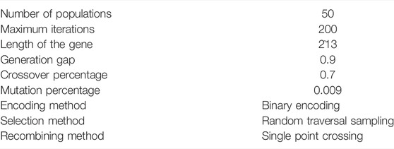
TABLE 4. Methods and parameters of GA.

4.2 Results Without Convertibility Index Constraint

In this section, the results of the planning model without the CI constraint are presented. The IES planning results are shown in Table 5. After optimization, we can calculate the CI of the IES. The CI is calculated according to the number and capacity of energy conversion devices. The CI result is 1.2, and the total cost is 102.392 million yuan.

TABLE 5

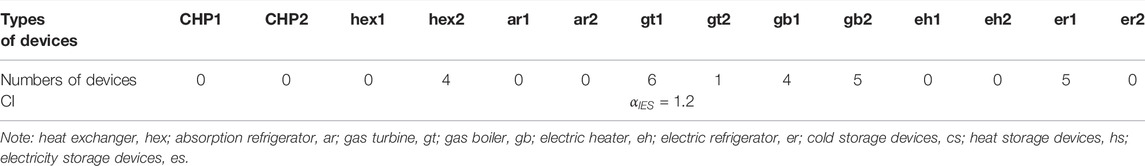
TABLE 5. Optimal planning results.

4.3 Results with Convertibility Index Constraint and Sensitivity Analysis

In order to analyze the results with different CIs, we used 10 cases with different CIs. The ${\alpha }_{\text{0}}$ in CI constraints is set from 0.7 to 1.6 with 0.1 steps in the 10 cases, respectively, as shown in Table 6.

TABLE 6

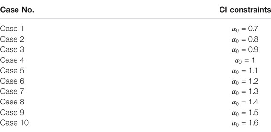
TABLE 6. Ten cases with different CIs.

Tables 7, 8 show the planning results of IES under different ${\alpha }_{\text{0}}$ in CI constraints. It can be seen that with the continuous increase in ${\alpha }_{\text{0}}$, the total number and capacities of conversion devices show an overall increase trend, but the increase is not strictly monotonous. Because of the integer variables in the planning problem, the planning results show non-linear changing trends. Moreover, with the continuous increase of CIs, the numbers of large-capacity devices also increases, except for the two types of electric heater. The reason is that the investment costs per unit power of the large-capacity device are a bit lower than that of small-capacity devices. As for the electric heaters, the number of electric heaters in the IES plan is small in all cases.

TABLE 7

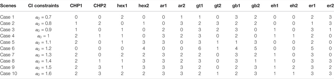
TABLE 7. Planning results with different CIs. (a) Numbers of each energy conversion device.

TABLE 8

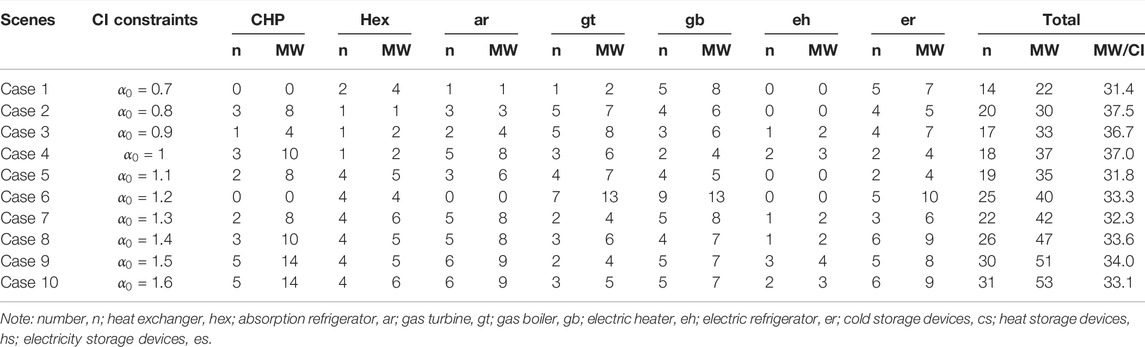
TABLE 8. Planning results with different CIs. (b) Numbers and capacities of each type of energy conversion device.

Table 9 shows the costs of IES planning results in different cases. The annual total cost with different CIs is shown in Figure 8. With the increase in the CIs, the annual total cost at first decreases quickly and then slightly increases, which on a whole shows a “Nike” shape. Compared with the result without CI constraint, when CI (${\alpha }_{\text{0}}$) decreases from 1.2 to 0.7, the annual total cost increases by 26.988 million yuan (26.2%), and when CI (${\alpha }_{\text{0}}$) increases from 1.2 to 1.6, the annual total cost increases by 3.841 million yuan (3.7%). The average cost increase for increasing per 0.1 CI is 2.229 million yuan (2.1%).

TABLE 9

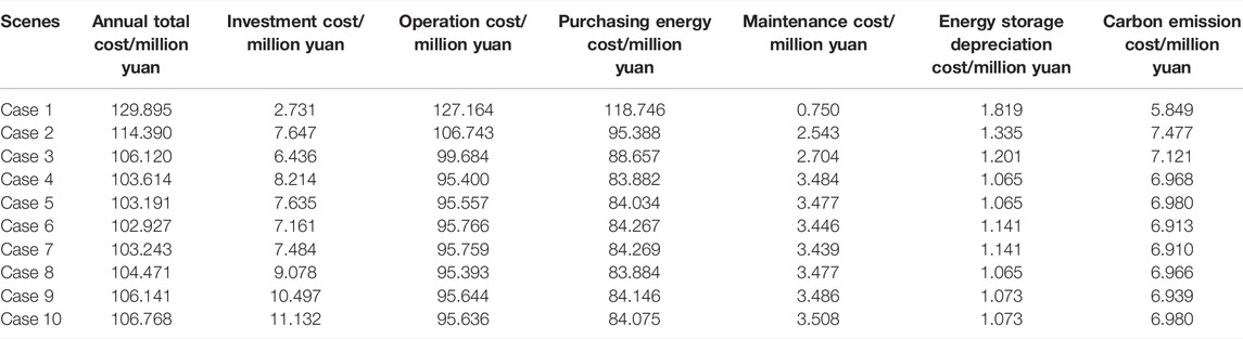
TABLE 9. Costs of planning schemes under the constraints of different CIs.

FIGURE 8

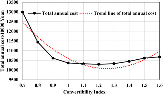
FIGURE 8. Annual total cost with different CIs.

Looking into the detailed results of the investment cost and operation cost, which are shown in Figures 9, 10, respectively, some more interesting results can be found. The results show that with the increase in the CI, the investment cost continuously increases gradually. When the CI (${\alpha }_{\text{0}}$) increases from 0.7 to 1.6, the investment cost increases by 307%. The reason is that the increase in CI leads to a rise in the number and capacity of energy conversion devices, and the investment cost therefore gradually increases. As for the operation cost, the results show that with the increase in the CI, the annual operation cost at first quickly decreases and then remains stable. When focusing the results from 0.7 to 1 of the CI, the higher flexibilities brought by adding energy conversion devices leave a larger feasible region for operation optimization. The IES, therefore, can take more advantage of the cheap energy conversion devices and save the annual operation cost. When focusing the results from 1 to 1.6 of the CI, the added flexibility is somewhat redundant and cannot help reduce the operation cost, and therefore the operation cost remains stable.

FIGURE 9

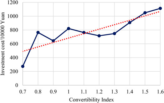
FIGURE 9. Investment cost with different CIs.

FIGURE 10

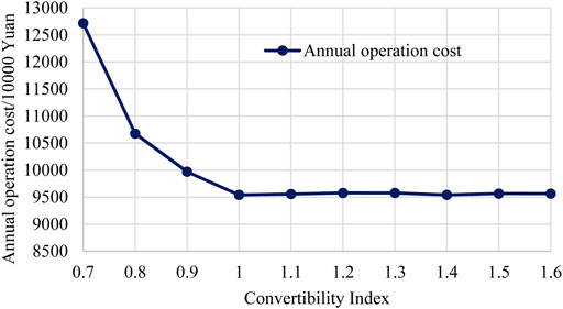
FIGURE 10. Annual operation cost with different CIs.

4.4 Performance of the Algorithm

The experiments are performed on a Windows-based server at Key Laboratory of Measurement and Control of Complex Systems of Engineering with an Intel(R) i7-9800X CPU (8 cores and 16 threads) and 32 GB of RAM. The hybrid GA–MILP solving algorithm was carried out in MATLAB, GAMS, and ILOG/CPLEX. The average solving time is 10653s. The bi-level planning annual total cost curve is shown in Figure 11. After nearly 120 iterations, the optimal annual total cost is 102.392 million yuan.

FIGURE 11

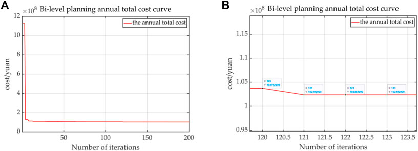
FIGURE 11. Bi-level planning annual total cost curve. (A) Overall convergence curve of the annual total cost. (B) After 120 times of convergence, the convergence value is obtained.

5 Conclusion and Discussion

This study proposes a new index—CI—to quantitatively assess the conversion flexibility of an IES system and builds up a planning problem for the IES with consideration of the impacts of the CI.

The main results of this study are as follows: 1) compared with the results without CI constraint, the CI constraints will increase the total cost. For the given case, the total cost increases by 26.2% when the CI decreases to 0.7 and increases by 3.7% when the CI increases to 1.6. With the continuous increase in the CI, the total cost at first decreases quickly and then slightly increases, which on a whole shows a “Nike” shape. 2) With the continuous increase in the CI, the total numbers and capacities of the conversion devices show an overall increase trend. When the CI increases from 0.7 to 1.6, the total number of the conversion devices increases by 121%, while the total capacity increases by 141%. 3) For the optimal results with different CIs, the MW per CI ranges from 31.8 to 37.5 MW, and the average cost increase is 2.229 million yuan (2.1%/0.1 CI). 4) The problem can be solved within 120 times iterations.

The advantages of the proposed methods are as follows: 1) the proposed index places the emphasis on flexibility assessment regarding the energy conversion process between different energy flow types, which can reflect the overall conversion flexibility of the IES. 2) The planner can obtain the most cost-saving IES plans and meet their CI requirement with CI constraints. The disadvantages of the proposed method are as follows: 1) the planning model is based on several assumptions, for example, the changes in the parameters with the operation status are neglected; and 2) the GA-based algorithm cannot ensure global optimum and is time consuming. The future research direction will be two-folded: 1) considering more practical issues in the planning problem, for example, using a practical system with real system data for simulation; and 2) exploring more efficient modeling and solving algorithms, for example, modeling it as a dual-objective optimization problem with the largest CI and the smallest annual total cost to find the Pareto surface.

Data Availability Statement

The original contributions presented in the study are included in the article/Supplementary Material, further inquiries can be directed to the corresponding author.

Author Contributions

Conceptualization: KZ; methodology: YW; software: FK; validation: TZ; writing: YW, KF and JZ; funding acquisition: KZ. All authors have read and agreed to the published version of the manuscript.

Funding

This study received funding from the National Natural Science Foundation of China (No. 51907025) and “Zhishan Young Scholar” of Southeast University (No. 2242021R41176). The funder was not involved in the study design, collection, analysis, interpretation of data, the writing of this article, or the decision to submit it for publication.

Conflict of Interest

Author TZ was employed by the company NARI Group Corporation (State Grid Electric Power Research Institute).

The remaining authors declare that the research was conducted in the absence of any commercial or financial relationships that could be construed as a potential conflict of interest.

Publisher’s Note

All claims expressed in this article are solely those of the authors and do not necessarily represent those of their affiliated organizations, or those of the publisher, the editors and the reviewers. Any product that may be evaluated in this article, or claim that may be made by its manufacturer, is not guaranteed or endorsed by the publisher.

Footnotes

¹Data [Online] is available at: https://github.com/wangyingrice/IES_planning.git.

References

Clegg, S., and Mancarella, P. (2016). Integrated Electrical and Gas Network Flexibility Assessment in Low-Carbon Multi-Energy Systems. IEEE Trans. Sustain. Energ. 7 (2), 718–731. doi:10.1109/TSTE.2015.2497329

CrossRef Full Text | Google Scholar

Coelho, A., Soares, F., and Peças Lopes, J. (2020). Flexibility Assessment of Multi-Energy Residential and Commercial Buildings. Energies 13 (11), 2704. doi:10.3390/en13112704

CrossRef Full Text | Google Scholar

Fan, H., Yu, Z., Xia, S., and Li, X. (2021). Review on Coordinated Planning of Source-Network-Load-Storage for Integrated Energy Systems. Front. Energ. Res. 9, 138. doi:10.3389/fenrg.2021.641158

CrossRef Full Text | Google Scholar

Farrokhifar, M., Nie, Y., and Pozo, D. (2020). Energy Systems Planning: A Survey on Models for Integrated Power and Natural Gas Networks Coordination. Appl. Energ. 262, 114567. doi:10.1016/j.apenergy.2020.114567

CrossRef Full Text | Google Scholar

Good, N., and Mancarella, P. (2019). Flexibility in Multi-Energy Communities with Electrical and thermal Storage: A Stochastic, Robust Approach for Multi-Service Demand Response. IEEE Trans. Smart Grid 10, 503–513. doi:10.1109/TSG.2017.2745559

CrossRef Full Text | Google Scholar

Grefenstette, J. J. (1988). Genetic Algorithms and Machine Learning. Machine Learn. 3 (2), 95–99. doi:10.1023/A:1022602019183

CrossRef Full Text | Google Scholar

Huang, W., Du, E., Capuder, T., Zhang, X., Zhang, N., Strbac, G., et al. (2021). Reliability and Vulnerability Assessment of Multi-Energy Systems: An Energy Hub Based Method. IEEE Trans. Power Syst. 36, 3948–3959. doi:10.1109/TPWRS.2021.3057724

CrossRef Full Text | Google Scholar

ILOG CPLEX. Homepage (2018). Available at: http://www.ilog.com (Accessed October 10, 2019).

Google Scholar

Jiang, Y., Wan, C., Botterud, A., Song, Y., and Xia, S. (2020). Exploiting Flexibility of District Heating Networks in Combined Heat and Power Dispatch. IEEE Trans. Sustain. Energ. 11 (4), 2174–2188. doi:10.1109/TSTE.2019.2952147

CrossRef Full Text | Google Scholar

Jie, D., Fei, J., Wenye, W., Guixiong, H., and Xinhe, Z. (2021). Study on Cascade Optimization Operation of Park-Level Integrated Energy System Considering Dynamic Energy Efficiency Model. Power Syst. Techn. 46 (03), 1027–1039. doi:10.13335/j.1000-3673.pst.2021.0484

CrossRef Full Text | Google Scholar

Jing, R., Zhu, X., Zhu, Z., Wang, W., Meng, C., Shah, N., et al. (2018). A Multi-Objective Optimization and Multi-Criteria Evaluation Integrated Framework for Distributed Energy System Optimal Planning. Energ. Convers. Manage. 166, 445–462. doi:10.1016/j.enconman.2018.04.054

CrossRef Full Text | Google Scholar

Koltsaklis, N. E., and Knápek, J. (2021). Optimal Scheduling of a Multi-Energy Microgrid. Chem. Eng. Trans. 88, 901–906. doi:10.3303/CET2188150

CrossRef Full Text | Google Scholar

Koltsaklis, N. E., Kopanos, G. M., and Georgiadis, M. C. (2014). Design and Operational Planning of Energy Networks Based on Combined Heat and Power Units. Ind. Eng. Chem. Res. 53 (44), 16905–16923. doi:10.1021/ie404165c

CrossRef Full Text | Google Scholar

Lannoye, E., Flynn, D., and O'Malley, M. (2012). Evaluation of Power System Flexibility. IEEE Trans. Power Syst. 27 (2), 922–931. doi:10.1109/TPWRS.2011.2177280

CrossRef Full Text | Google Scholar

Lei, Y., Wang*, D., Jia*, H., Chen, J., Li, J., Song, Y., et al. (2020). Multi-objective Stochastic Expansion Planning Based on Multi-Dimensional Correlation Scenario Generation Method for Regional Integrated Energy System Integrated Renewable Energy. Appl. Energ. 276. doi:10.46855/2020.06.11.05.59.391937

CrossRef Full Text | Google Scholar

Ma, J., Silva, V., Belhomme, R., Kirschen, D. S., and Ochoa, L. F. (2013). Evaluating and Planning Flexibility in Sustainable Power Systems. IEEE Trans. Sustain. Energ. 41, 200–209. doi:10.1109/tste.2012.2212471

CrossRef Full Text | Google Scholar

Ma, T., Wu, J., Hao, L., Lee, W.-J., Yan, H., and Li, D. (2018). The Optimal Structure Planning and Energy Management Strategies of Smart Multi Energy Systems. Energy 160, 122–141. doi:10.1016/j.energy.2018.06.198

CrossRef Full Text | Google Scholar

Mancarella, P. (2014). MES (Multi-energy Systems): An Overview of Concepts and Evaluation Models. Energy 65, 1–17. doi:10.1016/j.energy.2013.10.041

CrossRef Full Text | Google Scholar

Mendes, G., Ioakimidis, C., and Ferrão, P. (2011). On the Planning and Analysis of Integrated Community Energy Systems: A Review and Survey of Available Tools. Renew. Sustain. Energ. Rev. 15 (9), 4836–4854. doi:10.1016/j.rser.2011.07.067

CrossRef Full Text | Google Scholar

Mirakyan, A., and De Guio, R. (2013). Integrated Energy Planning in Cities and Territories: A Review of Methods and Tools. Renew. Sustain. Energ. Rev. 22, 289–297. doi:10.1016/j.rser.2013.01.033

CrossRef Full Text | Google Scholar

Mirakyan, A., and De Guio, R. (2015). Modelling and Uncertainties in Integrated Energy Planning. Renew. Sustain. Energ. Rev. 46, 62–69. doi:10.1016/j.rser.2015.02.028

CrossRef Full Text | Google Scholar

Nicolosi, F. F., Alberizzi, J. C., Caligiuri, C., and Renzi, M. (2021). Unit Commitment Optimization of a Micro-grid with a MILP Algorithm: Role of the Emissions, Bio-Fuels and Power Generation Technology. Energ. Rep. 7, 8639–8651. doi:10.1016/j.egyr.2021.04.020

CrossRef Full Text | Google Scholar

Nosair, H., and Bouffard, F. (2015). Flexibility Envelopes for Power System Operational Planning. IEEE Trans. Sustain. Energ. 6 (3), 800–809. doi:10.1109/TSTE.2015.2410760

CrossRef Full Text | Google Scholar

Pan, G., Gu, W., Lu, Y., Qiu, H., Lu, S., and Yao, S. (2020). Optimal Planning for Electricity-Hydrogen Integrated Energy System Considering Power to Hydrogen and Heat and Seasonal Storage. IEEE Trans. Sustain. Energ. 11, 2662–2676. doi:10.1109/TSTE.2020.2970078

CrossRef Full Text | Google Scholar

Qin, C., Yan, Q., and He, G. (2019). Integrated Energy Systems Planning with Electricity, Heat and Gas Using Particle Swarm Optimization. Energy 188, 116044. doi:10.1016/j.energy.2019.116044

CrossRef Full Text | Google Scholar

Shu, J., Guan, R., Wu, L., and Han, B. (2019). A Bi-level Approach for Determining Optimal Dynamic Retail Electricity Pricing of Large Industrial Customers. IEEE Trans. Smart Grid 10 (2), 2267–2277. doi:10.1109/TSG.2018.2794329

CrossRef Full Text | Google Scholar

Su, H., Huang, Q., and Wang, Z. (2021). An Energy Efficiency Index Formation and Analysis of Integrated Energy System Based on Exergy Efficiency. Front. Energ. Res. 9. doi:10.3389/fenrg.2021.723647

CrossRef Full Text | Google Scholar

Wang, J., Du, W., and Yang, D. (2021). Integrated Energy System Planning Based on Life Cycle and Emergy Theory. Front. Energ. Res. 9, 713245. doi:10.3389/fenrg.2021.713245

CrossRef Full Text | Google Scholar

Wang, J., Hu, Z., and Xie, S. (2019c). Expansion Planning Model of Multi-Energy System with the Integration of Active Distribution Network. Appl. Energ. 253, 113517. doi:10.1016/j.apenergy.2019.113517

CrossRef Full Text | Google Scholar

Wang, Y., Huang, F., Tao, S., Ma, Y., Ma, Y., Liu, L., et al. (2022). Multi-objective Planning of Regional Integrated Energy System Aiming at Exergy Efficiency and Economy. Appl. Energ. 306, 118120. doi:10.1016/j.apenergy.2021.118120

CrossRef Full Text | Google Scholar

Wang, Y., Li, R., Dong, H., Ma, Y., Yang, J., Zhang, F., Zhu, J., and Li, S. (2019a). Capacity Planning and Optimization of Business Park-Level Integrated Energy System Based on Investment Constraints. Energy 189, 116345. doi:10.1016/j.energy.2019.116345

CrossRef Full Text | Google Scholar

Wang, Y., Wang, Y., Huang, Y., Li, F., Zeng, M., Li, J., et al. (2019b). Planning and Operation Method of the Regional Integrated Energy System Considering Economy and Environment. Energy 171, 731–750. doi:10.1016/j.energy.2019.01.036

CrossRef Full Text | Google Scholar

Wenxia, L., Zhengzhou, L., Yue, Y., Fang, Y., and Yao, W. (2020). Collaborative Optimal Configuration for Integrated Energy System Considering Uncertainties of Demand Response. Automation Electric Power Syst. 44 (10), 9. doi:10.7500/AEPS20190731013

CrossRef Full Text | Google Scholar

Xiang, Y., Cai, H., Gu, C., and Shen, X. (2020). Cost-benefit Analysis of Integrated Energy System Planning Considering Demand Response. Energy 192, 116632. doi:10.1016/j.energy.2019.116632

CrossRef Full Text | Google Scholar

Xiao, H., Pei, W., Pei, W., Dong, Z., and Kong, L. (2018). Bi-level Planning for Integrated Energy Systems Incorporating Demand Response and Energy Storage under Uncertain Environments Using Novel Metamodel. Csee Jpes 4 (2), 155–167. doi:10.17775/CSEEJPES.2017.01260

CrossRef Full Text | Google Scholar

Zhang, X., Wang, H., Hu, J., Zhou, B., Zhang, Y., and Qiu, J. (2019). Game-theoretic Planning for Integrated Energy System with Independent Participants Considering Ancillary Services of Power-To-Gas Stations. Energy 176, 249–264. doi:10.1016/j.energy.2019.03.154

CrossRef Full Text | Google Scholar

Zheng, T., Dai, Z., Yao, J., Yang, Y., and Cao, J. (2019). Economic Dispatch of Multi-Energy System Considering Load Replaceability. Processes 7, 570. doi:10.3390/pr7090570

CrossRef Full Text | Google Scholar

Zhou, X., Yonghui, S., Dongliang, X., Jianxi, W., and Yongjie, Z. (2020). Optimal Configuration of Energy Storage for Integrated Region Energy System Considering Power/Thermal Flexible Load. Automation Electric Power Syst. 44 (2), 7. doi:10.7500/AEPS20190620005

CrossRef Full Text | Google Scholar

Zhou, Z., Liu, P., Li, Z., and Ni, W. (2013). An Engineering Approach to the Optimal Design of Distributed Energy Systems in China. Appl. Therm. Eng. 53, 387–396. doi:10.1016/j.applthermaleng.2012.01.067

CrossRef Full Text | Google Scholar