View Factors in Horizontal Plane Fixed-Mode Solar PV Fields

In solar PV fields, solar photovoltaic panels are typically arranged in parallel rows one after the other. This arrangement introduces variations in the distribution of solar irradiance over the entire field, compared to measurements recorded at meteorological weather stations and data obtained from climatic database platforms. This is due to the difference in the view factors between the rows of the solar PV field and a single surface, as well as the presence of shade on rear sides and in the space separating the rows. These phenomena combined will reduce the intensity of solar irradiance incident on the PV solar field; consequently will reduce the energy yields. Accurate estimation of solar radiation on solar fields requires knowledge of the sky, ground, and rear side of the preceding row view factors, and an estimation of the time and space occupied by the row’s shadow. Prior literature has addressed this issue using two-dimensional (2-D) techniques such as the crossed-strings method (CSM). This study developed a novel three-dimensional (3-D) analysis in addition to numerical analysis to determine the view factors associated with solar fields. The study uses both isotropic and anisotropic transposition analyses to determine solar irradiance incident on the solar field with varying tilt angles of solar panels and distance separating the rows (distance aspect ratio) for several latitudes. The present research also tested the validity of the CSM for wide ranges of distance separating rows and length aspect ratios, the obtained results show that the CSM shows good agreements in both sky and ground view factor in the range of length aspect ratio greater than one. But the CSM fails in rear-side view factor in the design ranges of PV solar fields, where the error rate was found about 11%, this result is important in the case of bifacial PV solar systems. Also, the present work compared the solar irradiance calculated for a single surface with that incident on a PV solar field for wide range of sky conditions and latitudes. The obtained results ensure the accuracy of using the solar irradiance incident on a single surface data for low latitudes and for most sky conditions for PV rooftop solar systems as well as PV solar fields. While it has remarked a large error in the case of cloudy skies, where the error rate exceeded 17% in the case of aspect ratio equals to 1.5 and about 15.5% in the aspect ratio of 2.0.

1 Introduction

The performance prediction of any engineering system is an important step in the designing process, especially in solar fields (thermal or photovoltaic). As it is important to estimate the sizing of solar panels, number of rows, distance separating rows, and tilt and azimuth angles of the panels (Nassar, 2006; Alsadi and Nassar, 2017a; Seme et al., 2019). The solar irradiation incident on a tilted single surface consists from three components; direct beam, sky diffuse, and ground-reflected solar irradiation. While the situation in the solar fields is different, excluding the first row of solar panels in the solar filed, the solar radiation on the rest of panels consists of direct beam, sky diffuse, ground reflected, and rear surface reflected irradiation. The amounts of the sky diffuse, ground reflected, and rear surface-reflected irradiation captured by the PV panels depend on the view factor of panels to sky, ground, and rear surface (Nassar, 2006; Appelbaum, 2018). The view factors are used commonly in analyzing radiative heat transfer of many energy engineering applications. An online compilation of view factors for over 300 common geometries is provided by Howell (2016), and the list is regularly updated with new geometries. View factor plays a crucial role in transferring irradiances from horizontal planes to tilted planes (Arias-Rosales and LeDuc, 2020; Nassar et al., 2020). A recently developed numerical–analytical model by Nassar (2020) is used to facilitate the simulation of all types of solar fields. The sky diffuse transposition models are considered as examples of view factor models (Arias-Rosales and LeDuc, 2020), several models are presented in literature to measure the sky diffuse view factor, that is, Liu-Jordan, Klucher, Perez, Hay, and Reindl models (Mubarak et al., 2017). The Liu-Jordan model is considered the most prominent and oldest definitions (Liu and Jordan, 1961).

In the literature, several studies have performed, in which the view factor is used to estimate the diffuse radiation. Alam et al (2019) performed a numerical comparison study applied to several building depending on the view factor where radiative exchange takes place between surfaces such as ground and vertical walls or ground and sloping thermal or photovoltaic collectors. Alsadi and Nassar (2017a) performed a theoretical study using the view factor to analyze the solar field with a fixed reflector placed on the back-side top of the preceding row. Appelbaum (2018) presented an analytical expressions and numerical values of view factors between collectors to sky, between opposite collectors, and between collectors to shaded and not shaded grounds, for the front and rear sides of the collectors deployed on the horizontal and inclined planes. The complexity in handling the ground albedo for the entire solar field compared to a single-row array or the first row of a solar field arose from the inherent differences in the sky and ground view factors among the solar field rows and the presence of shadows in the space separating the rows was discussed in Alsadi and Nassar (2017b); Alsadi and Nassar (2019).

To numerically solve the assigned model, various authors derived different methods to calculate the view factor. But the most commonly used methods are as follows: 1) direct integration method; 2) unit sphere method; 3) ray casting method; 4) cross string method; 5) Monte Carlo method; and 6) algebraic rule and matrix formulation (Gupta et al., 2017). Among all the aforementioned techniques, the crossed-string method (CSM) is the most widely used to determine the view factors of the sky and the ground as seen by the rows of the solar PV field (Alsadi and Nassar, 2016; Alsadi and Nassar, 2017b; Appelbaum, 2018).

Most studies relating to view factors were reviewed in Appelbaum (2018). View factors of PV panels on rooftops of buildings were reported in Appelbaum and Aronescu (2016), and view factors of solar collectors deployed on horizontal, inclined, and step-like planes were discussed in Nassar and Alsadi (2016). All previously mentioned studies addressed the solar PV field as a two-dimensional problem. In general, two-dimensional analysis is based on the hypothesis that the length of a row is infinitely longer than its height (Appelbaum and Aronescu, 2016). Although this assumption might be considered reasonable for large solar PV fields, the same cannot be said for rooftop solar PV installations. The installation of solar PV on rooftops of buildings is becoming more widespread and can be a solution to the energy problem in many countries (Nassar and Alsadi, 2019).

The present study distinguishes from its predecessors is the use of three-dimensional analysis to address the problem comprehensively, making it applicable to any type of solar field. A key finding of this work is the outline of two approaches to estimate solar irradiance incident on solar field rows for isotropic and anisotropic skies, something that has not thus far been studied, to the best of our knowledge. This represents the significance of the present research.

The rest of the article is further organized as follows: the theoretical framework of the study is outlined in section 2. The obtained results have been demonstrated graphically by several means and discussed in section 3. While section 4 deals with the calculation of the solar irradiation incident on a solar field located in Tripoli city, Libya and Ankara city, Turkey as case studies for low and high latitudes sites. The conclusions drawn from the research are outlined in Section 5. Finally, the study is finished with a list of cited works.

2 Mathematical Modeling

In this section, the mathematical modeling of the problem is presented. It starts with defining the view factors, and then followed by introducing the analysis of the two-dimensional (2-D) and three-dimensional (3-D) view factors.

2.1 Definition and Algebra of the View Factors

In the literature, the view factor $F_{A_i-A_j}$ is defined as the fraction of radiation leaving surface $A_i$ that is directly striking surface $A_j$ (Vujičić et al., 2016). The view factor has properties that are important in analyzing and solving view factor problems, which are expressed as follows (Baehr and Karl, 2011):

$A_i{F}_{A_i-A_j}=A_j{F}_{A_j-A_i}\left(\text{The reciprocity rule}\right),(1)$

${\displaystyle \sum }_{j=1}^N{F}_{A_i-A_j}=1\left(\text{The summation rule}\right),(2)$

$F_{A_i-(A_{j1}+A_{j2})}=F_{A_i-A_{j1}}+F_{A_i-A_{j2}}\left(\text{The superposition rule}\right).(3)$

2.2 Two-Dimensional (2-D) Approach for Calculation of the View Factors

In this work, the crossed-strings method (CSM) approach is considered for two-dimensional (2-D) analysis of view factors. CSM is considered as a widely used approach for 2-D analysis. In particular, CSM is applied to geometries that are very long in one direction relative to the other directions. By attaching strings between corners, as illustrated in Figure 1, the view factor between two surfaces can be expressed as follows (Nassar and Alsadi, 2016):

$\begin{array}{l}{F}_{i\to j}=\frac{\sum crossed strings-\sum uncrossed strings}{2\times string on surface i},\mathrm{so}\\ F_{A_2\to A_1}=\frac{\left[\overline{be}+\overline{ac}\right]-\left[\overline{bc}+\overline{ae}\right]}{2\overline{ec}}.\end{array}(4)$

FIGURE 1

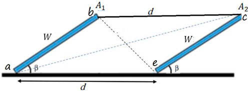
FIGURE 1. Definition of the crossed-strings method for two surfaces of infinite length.

According to this definition, the view factors may be derived and expressed as follows (Nassar and Alsadi, 2016):

$F_{A_1\to s}=\frac{1+cos\beta }{2},(5)$

$F_{A_1\to g}=\frac{1-cos\beta }{2},(6)$

$F_{A_2\to s}=\frac{1}{2}\left[1+\frac{d}{W}-\sqrt{{\left(\frac{d}{W}-cos\beta \right)}^2+{\left(sin\beta \right)}^2}\right],(7)$

$F_{A_2\to g}=\frac{1}{2}\left[1+\frac{d}{W}-\sqrt{{\left(\frac{d}{W}+cos\beta \right)}^2+{\left(sin\beta \right)}^2}\right],(8)$

$F_{A_1\to A_{1r}}=\frac{1}{2}\left[\sqrt{{\left(\frac{d}{W}-cos\beta \right)}^2+{\left(sin\beta \right)}^2}+\sqrt{{\left(\frac{d}{W}+cos\beta \right)}^2+{\left(sin\beta \right)}^2}-2\frac{d}{W}\right].(9)$

In the earlier mentioned relations, $F_{A_1\to s}$ is the first row to the sky view factor, $F_{A_1\to g}$ is the first row to the ground view factor, $F_{A_2\to s}$ is second and the succeeding rows to the sky view factor, $F_{A_2\to g}$ is second and the succeeding rows to the ground view factor, and $F_{A_1\to A_{1r}}$ is the second row to rear surface of the first row view factor. Considering the length of the solar panels (L), the view factor can be calculated for different designs.

2.3 Three-Dimensional (3-D) Approach for Calculation of View Factors

For further improvement of predicated energy yields, costs, and optimum design, a 3-D analysis is adopted to accurately calculate view factors of solar PV fields. A schematic diagram for a successive solar collector in a solar field is shown in Figure 2. Figure 2 displays all view factors that are associated with a horizontal plane PV field at an instant of time, which will be the reference to the rest of the discussion. All the nomenclature of view factors that is related to a horizontal plane fixed-mode solar PV field at any moment of time is also displayed in Figure 2.

FIGURE 2

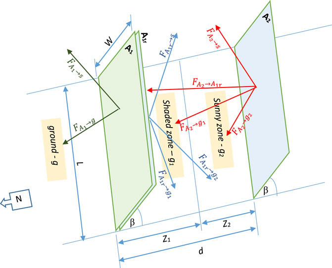
FIGURE 2. View factors of a horizontal plane solar PV field at an instant of time.

For further analysis, the view factor expressions in Nassar (2020) have been reformed to match the geometry of the solar PV field depicted in Figure 2, as displayed in Table 1. It is worth mentioning that the multi-integration expressions in Table 1 have no mathematical solution yet and can be evaluated via numerical techniques only.

TABLE 1

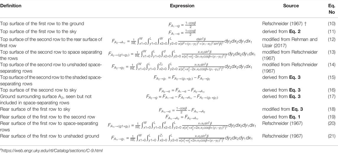
TABLE 1. Expressions for view factors depicted in Figure 2.

The integrals in Eq. 12–14, 20, 21 are partially solved with one term remaining unsolved. The unsolved term is solved in this work numerically by means of the Gaussian quadrature five-point rule as shown in Appendix A1.

2.4 Calculation of Shadow in Space-Separating Rows

In solar PV fields, shadow has a great effect on the ground view factor for the second and subsequent rows. Figure 3 presents a schematic for two plates in subsequent rows where the distance separates the rows (d) has the shaded zone (Z₁) and the unshaded zone (Z₂). For the solar field, the estimation of the effect of shadow is extensively studied (Groumpos and Khouzam, 1987; Nassar et al., 2008; Alsadi and Nassar, 2019). A general expression for shadow geometry in all types of solar fields is given in Alsadi and Nassar (2019). In Figure 3, it can be seen that the length of the shadow in the space separating the rows is much longer than its width. Thus, it can be assumed that the shadow is of rectangle shape, resulting in simplifying the problem without significant effect on the results.

FIGURE 3

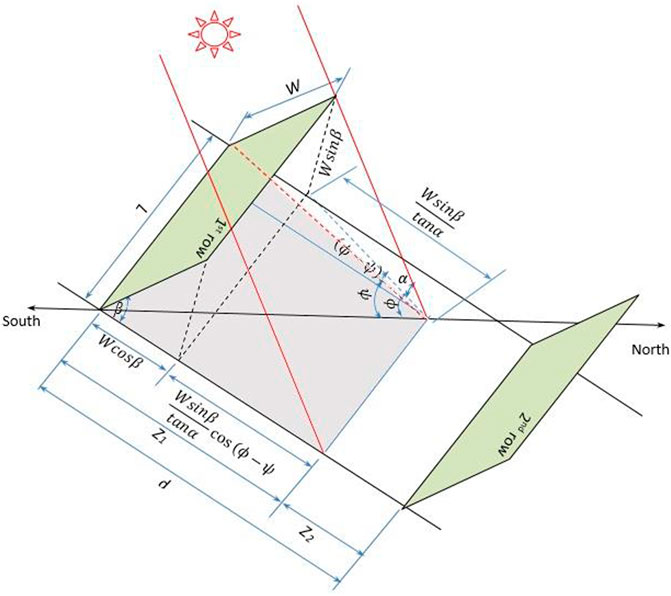
FIGURE 3. Graphical representation of the shaded and unshaded zones in a solar field.

Eq. 22 and 23 present the shaded g₁ and unshaded g₂ zone lengths in terms of dimensionless ratio of lengths Z₁ and Z₂ of the shaded and unshaded zones with respect to the distance separating the rows (d).

$\frac{Z_1}{d}=\frac{W}{d}cos\beta +\frac{W}{d}\frac{sin\beta }{tan\alpha }cos\left(\varnothing -\psi \right)if\{\begin{array}{c}\frac{Z_1}{d}<0; \frac{Z_1}{d}=0\\ \frac{Z_1}{d}>1; \frac{Z_1}{d}=1\end{array}(22)$

$\frac{Z_2}{d}=1-\frac{Z_1}{d}if\{\begin{array}{c}\frac{Z_2}{d}<0; \frac{Z_2}{d}=0\\ \frac{Z_2}{d}>1; \frac{Z_2}{d}=1\end{array}.(23)$

3 Results and Discussion

3.1 First Row View Factors

To determine the incident solar radiation on the first row of a solar field and its view factor, it is treated as a single-tilted surface.

3.1.1 $F_{A_1\to g}$

The $F_{A_1\to g}$ presents the first row to the ground view factor in which g refers to the ground surface seen by the first-row surface A₁. Assuming the ground surface in front and on either sides of the first row is unshaded, the value of $F_{A_1\to g}$ is constant and depends only on the row tilt angle β, which can be calculated by Eq. 10. Eq. 10 shows that $F_{A_1\to g}$ is directly proportional to the tilt angle β.

3.1.2 ${\mathit{F}}_{{\mathit{A}}_1\to \mathit{s}}$

The $F_{A_1\to s}$is the first row to sky view factor. It has a constant value and can only be affected by the row tilt angle β. It is clear from Eq. 11 that $F_{A_1\to s}$ is inversely proportional to the tilt angle β.

3.2 Second Row View Factors

Numerous values of the second row view factors’ contour representation are plotted in Figures 4–7.

FIGURE 4

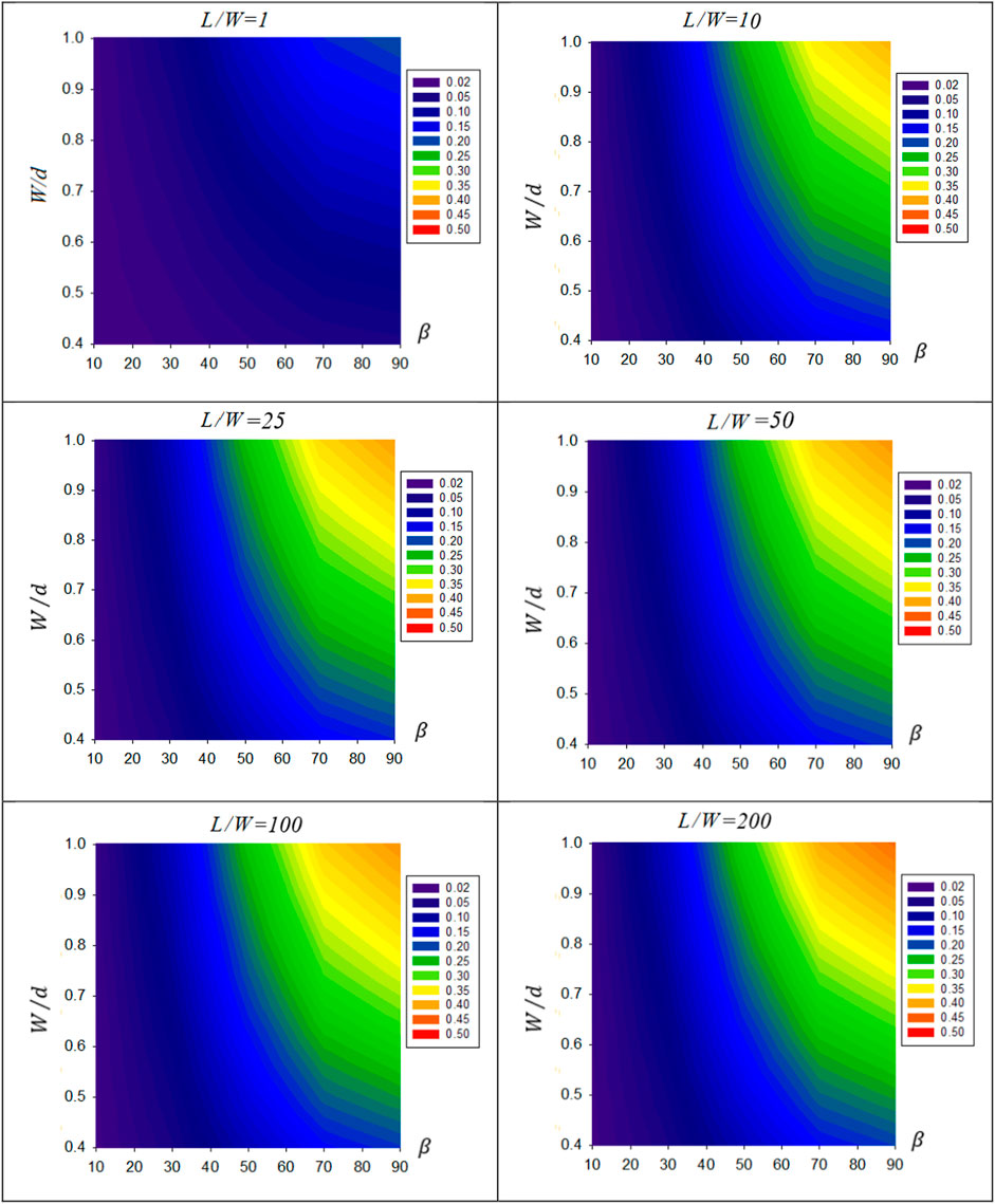
FIGURE 4. Contour representation of $F_{A_2\to A_{1r}}$ as a function of the aspect ratio $\frac{W}{d}$ and row tilt angle β, for various values of the aspect ratio $\frac{L}{W}$.

3.2.1 ${\mathit{F}}_{{\mathit{A}}_2\to {\mathit{A}}_{1\mathit{r}}}$

The view factor ${\mathit{F}}_{{\mathit{A}}_2\to {\mathit{A}}_{1\mathit{r}}}$ represents the second row to the rear surface of the first row view factor. The view factor ${\mathit{F}}_{{\mathit{A}}_2\to {\mathit{A}}_{1\mathit{r}}}$ is displayed with respect to the design parameters of a solar PV field in a contour plot in Figure 4. Figure 5 demonstrates the relationship between $F_{A_2\to A_{1r}}$ and the field design parameters.

FIGURE 5

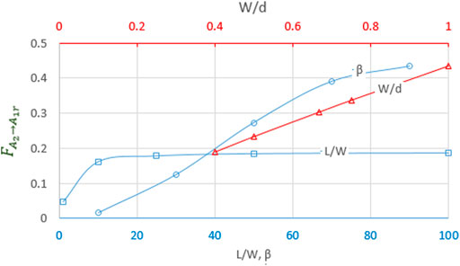
FIGURE 5. Influence of solar field design parameters on$F_{A_2\to A_{1r}}$

Figures 4, 5 show that increasing the tilt angle β leads to a significant increase in the view factor $F_{A_2\to A_{1r}}$ by a cubic order polynomial. Similarly, an increase in the value of $F_{A_2\to A_{1r}}$ is almost proportional to that of the aspect ratio $\frac{W}{d}$. On the other hand, the influence of the aspect ratio $\frac{L}{W}$ is limited to values < 10 as in the case of rooftop solar installation.

3.2.2 ${\mathit{F}}_{{\mathit{A}}_2\to ({\mathit{g}}_1+{\mathit{g}}_2)}$

In this section, the value of the view factor ${\mathit{F}}_{{\mathit{A}}_2\to ({\mathit{g}}_1+{\mathit{g}}_2)}$ is partially evaluated by numerically solving the multi-integral Eq. 13, with solving the remaining part using the Gaussian quadrature five-point rule (Appendix A1). Where the subscripts g₁ and g₂ refer to the shaded and unshaded zones, respectively. The contour plot (Figure 6) exhibits the effect of solar field design parameters on the value of ${\mathit{F}}_{{\mathit{A}}_2\to {\mathit{A}}_{1\mathit{r}}}.$ The result shows that the value of ${\mathit{F}}_{{\mathit{A}}_2\to ({\mathit{g}}_1+{\mathit{g}}_2)}$ is a constant, depending on solar field design parameters β and d.

FIGURE 6

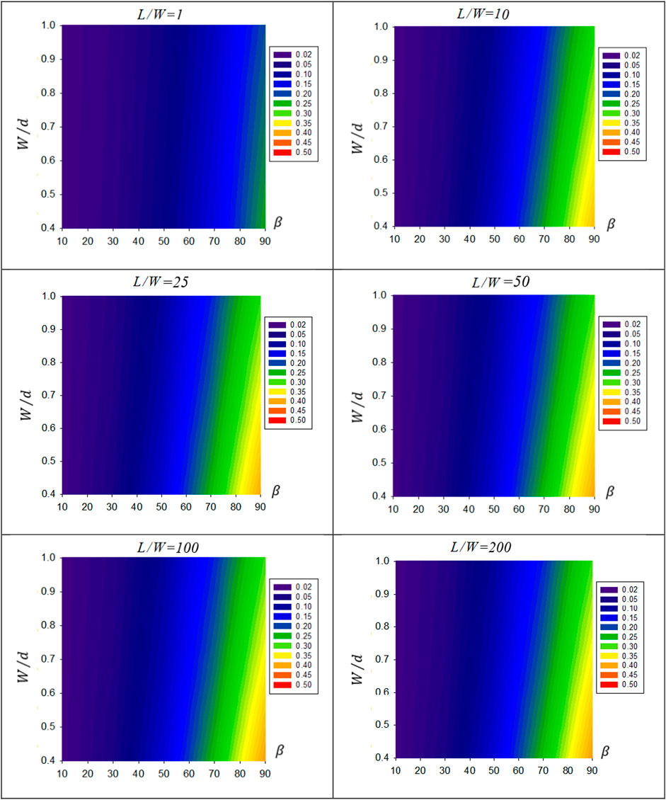
FIGURE 6. Contour representation of ${\mathit{F}}_{{\mathit{A}}_2\to ({\mathit{g}}_1+{\mathit{g}}_2)}$ as a function of the aspect ratio $\frac{W}{d}$ and row tilt angle β, for various values of aspect ratio $\frac{L}{W}$.

Figures 7, 8 show that as the row tilt angle β increases the value of the view factor $F_{A_2\to (g_1+g_2)}$ increases in a quadratic power polynomial scale. It also shows that the value of $F_{A_2\to (g_1+g_2)}$ decreases linearly as the value of the aspect ratio $\frac{W}{d}$ increases. On the other hand, as the length of the row for the aspect ratio $\frac{L}{W}$ increases from 0 to 10 leads to a large logarithmical scale increase in the value $F_{A_2\to (g_1+g_2)}$ and flattened beyond $\frac{L}{W}>10$ into a straight line having zero slope as depicted in Figure 7.

FIGURE 7

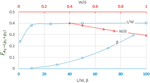
FIGURE 7. Influence of solar field design parameters on$F_{A_2\to (g_1+g_2)}$

FIGURE 8

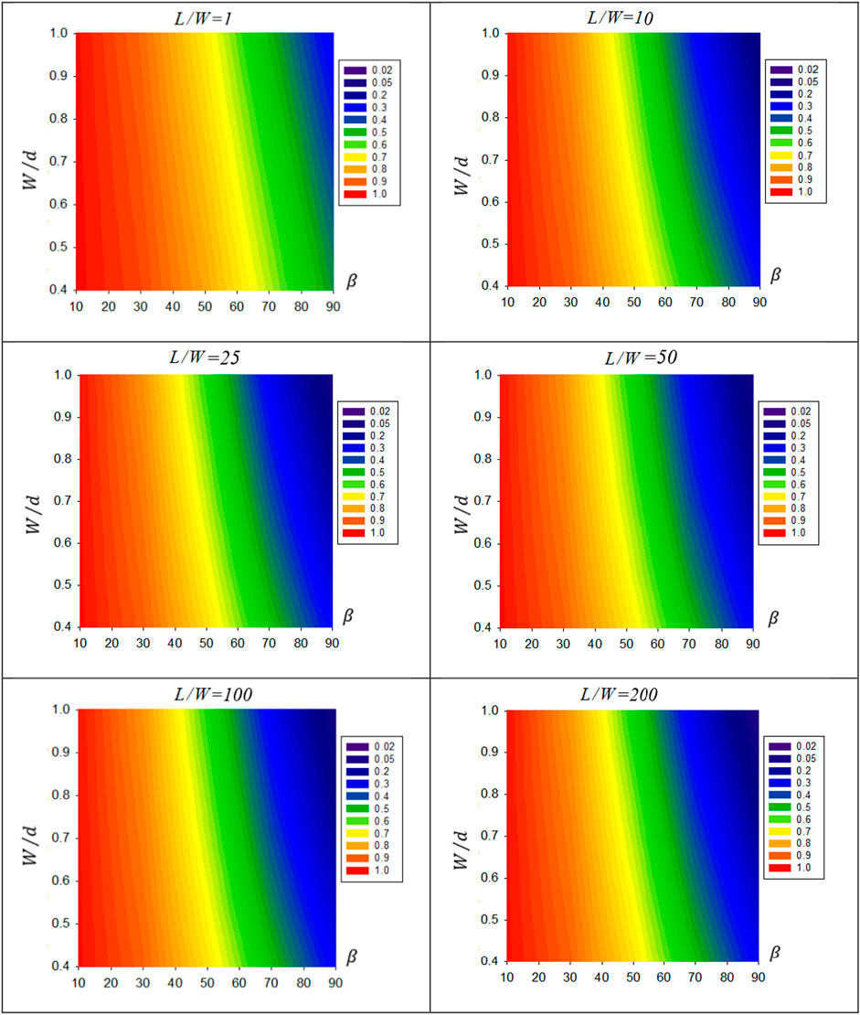
FIGURE 8. Contour representation of $F_{A_2\to s}$ as a function of $\frac{W}{d}$ , β, and $\frac{L}{W}$.

3.2.3 ${\mathit{F}}_{{\mathit{A}}_2\to \mathit{s}}$

The sky view factor ${\mathit{F}}_{{\mathit{A}}_2\to \mathit{s}}$ is one of the important factors for its relatively large effect on the contribution of sky diffuse irradiance to the total global tilted solar irradiation. Where under an overcast sky all irradiance is diffuse, while under a standard clear-sky, about 70% of global tilted irradiance is direct, 23% diffuse, and the rest is ground reflected (Nassar, 2005). The value of ${\mathit{F}}_{{\mathit{A}}_2\to \mathit{s}}$ can be obtained by applying the superposition rule. The second row sees the sky as the first row sees it (${\mathit{F}}_{{\mathit{A}}_1\to \mathit{s}}$) less the blocking that takes place due to the presence of the first row in front of it ($F_{A_2\to A_{1r}}$). Figure 8 is a contour plot showing the behavior of ${\mathit{F}}_{{\mathit{A}}_2\to \mathit{s}}$ when changing the design parameters of the solar PV field β, $\frac{W}{d}$ and $\frac{L}{W}$.

The row tilt angle β is a critical parameter in the sky view factor. It is found that as β increases the value of sky view factor reduces by a cubic order polynomial. Also, the value of the sky view factor is inversely proportional to the aspect ratio $\frac{W}{d}$. Furthermore, the length of row has an inverse power effect on the sky view factor for the low aspect ratio $\frac{L}{W}<10$, diminishing to have no effect for larger aspect ratios. Figure 9 demonstrates that for typical solar field applications, the sky view factor is affected only by row tilt angle.

FIGURE 9

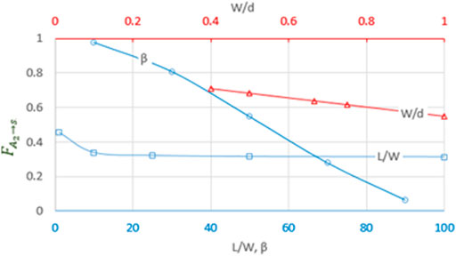
FIGURE 9. Influence of solar field design parameters on$F_{A_2\to s}$

3.2.4 ${\mathit{F}}_{{\mathit{A}}_2\to \mathit{g}}$

The subscript g refers to ground seen by the row, in front and on either side of it. The view factor ${\mathit{F}}_{{\mathit{A}}_2\to \mathit{g}}$ value is obtained using the summation rule that is subtracting the total second row view factors from that of the first row view factor. In this case, the total ground area is assumed to be unshaded. Figure 10 is a contour plot representing the relationship between ${\mathit{F}}_{{\mathit{A}}_2\to \mathit{g}}$ and the solar PV field’s design parameters β, $\frac{W}{d}$ and $\frac{L}{W}$.

FIGURE 10

FIGURE 10. Contour presentation of $F_{A_2\to g}$ as a function of β, $\frac{W}{d}$, and $\frac{L}{W}$.

Figure 10 shows that $F_{A_2\to g}$ is affected significantly by tilt angle β, and they have almost direct linear relationship. With respect to the aspect ratio $\frac{L}{W}$, the view factor $F_{A_2\to g}$ has a power function relationship for $\frac{L}{W}$ <10, leading to a sharp decrease in $F_{A_2\to g}$. For higher ratios, the relation diminishes to no effect. On the other hand, the aspect ratio W/d has a lesser effect being almost directly proportional to $F_{A_2\to g}$, as depicted in Figure 11.

FIGURE 11

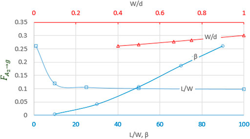
FIGURE 11. Influence of solar field design parameters on$F_{A_2\to g}$

3.3 Dynamic View Factors

The four view factors defined in this work are dynamic due to the fact that they depend on the shadow in the space between separating rows, and shadow is function of time and location, hence the name “dynamic.” As illustrated in Figure 2, the four view factors are as follows: view factor between the second row and the shaded zone g₁ $\left(F_{A_2\to g_1}\right)$, view factor between the second row and the unshaded zone g₂ $\left(F_{A_2\to g_2}\right)$, view factor between rear surface of the first row and the shaded zone g₁ $\left(F_{A_{1r}\to g_1}\right)$, and view factor between the rear surface of the first row and the unshaded zone g₂ $\left(F_{A_{1r}\to g_2}\right)$.

3.4 Calculation of Shadow

Shadow of an object depends on the design parameters, the location ($\varnothing$), and time assigned by solar altitude and azimuth angles α and γ, respectively. It is a well-known fact that shadow is longer at high latitudes, early in the morning, and late in the evening. The longest show occurs in winter solstice. It gets shorter at solar noon, reaching its shortest at summer solstice. In relation to PV fields, in addition to location and time, shadow depends on field dimensions and row tilt angle $\beta .$ Among these parameters, the most flexible and controllable parameter is the row tilt angle $\beta$ in order to influence the effect of shadow. The tilt angle $\beta$ was recommended not to exceed 30° for European installations (Vokony et al., 2018) while a tilt angle $\beta$ of about 20° was recommended for North Africa (Agha and Sbita, 2000; Alsadi et al., 2016). Figure 12 is a radar plot representing a comparison between two categories of locations: MENA with $\varnothing =30°, \beta =20°$ and Europe with $\varnothing =40°, \beta =30°$ for both longest and shortest shadows occurring on June 21st and December 21st, respectively, for several aspect ratios $\frac{W}{d}=0.5,0.667\text{ , and }1.0$.

FIGURE 12

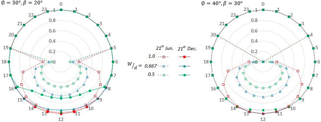
FIGURE 12. Comparison of the shadow zone length ratio $\frac{Z_1}{d}$ between two locations with different tilt angles on the 21st of summer and winter solstices. The aspect ratio $\frac{W}{d}$ is a parameter.

3.5 Comparison of View Factors of the Surface $F_{A_2}$ Obtained by CSM and 3-D Analysis

A comparison between second row surface view factors at different design parameters for CSM and 3-D analysis are presented in Figure 13. To produce Figure 2, Β is considered $30°$ and the view factor is calculated at different aspect ratios $\frac{d}{W}$ for various aspect ratios $\frac{L}{W}$ . Where the error between the two methods is calculated using Eq. 24.

$Error=\frac{F_{A_2} \left(CSM\right)-F_{A_2} \left(3D\right)}{F_{A_2} \left(CSM\right)}\times 100.(24)$

FIGURE 13

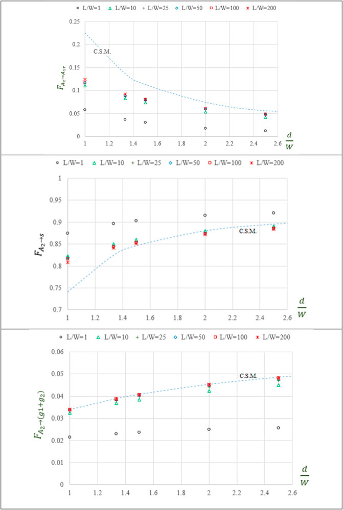
FIGURE 13. Comparison of view factors of surface $F_{A_2}$ obtained by CSM and 3-D analysis as a function of the aspect ratio $\frac{d}{W}$ for various aspect ratios $\frac{L}{W}$ and$\beta =30°$

It is found that for solar PV field with aspect ratios $\frac{d}{W}\approx 1.5$ and $\frac{L}{W}\approx 25$, the view factors estimate has errors of 3%, -1, and 44% for $F_{A_1\to s}$ , $F_{A_2\to g}$, and $F_{A_2\to A_{1r}}$, respectively. For rooftop solar PV installations with aspect ratios $\frac{d}{W}\approx 1.5$ and $\frac{L}{W}\approx 5$, the errors were found consecutively to be 30%, -6, and 38% for $F_{A_1\to s}$ , $F_{A_2\to g}$, and $F_{A_2\to A_{1r}}$. It should be noted that CSM produced a large $F_{A_2\to A_{1r}}$ error even for vertical planes compared with 3-D analysis. Applying Eq. 24 for the same solar field ($\frac{d}{W}\approx 1.5$ and $\frac{L}{W}\approx 25$), the errors produced due to the use of CSM are as high as 11% in the case of $F_{A_2\to A_{1r}}$.

The inherent restriction of CSM where the length of a solar field is assumed to be much longer than its width (i.e. $\frac{L}{W}\cong \infty$) is applicable only in large solar PV fields >100 MW. In comparison, smaller solar PV fields such as rooftop installation where the aspect ratio $\frac{L}{W}$ is relatively small (<5), the view factors estimate exhibit significantly larger errors.

3.6 Case Study

In this part, author presented a case study in Libyan. The results presented here are for a horizontal plane fixed-mode solar PV field project planned by the Libyan government in an effort to transition to electricity generation using abundant renewable energy resources available in the country. The project is located on the outskirts of the capital city Tripoli ($32.815°N, 13.439°E$). The solar PV field is orientated due south ($\psi =0$), having a tilt angle $\beta =20°$ from the horizontal, the rows dimensions $L\times W$ are $200\times 6$ m, with the rows placed 9 m apart.

Applying Eq. 22, 23 for the aforementioned solar field yielded the results depicted as in Figure 14, which is represented as a radar chart for the 21st of every month for both shaded and unshaded zones.

FIGURE 14

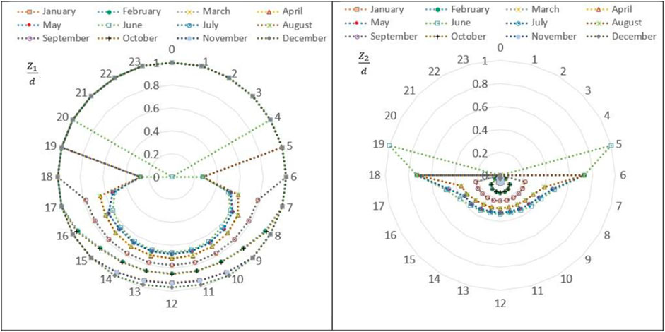
FIGURE 14. Aspect ratio of the shaded and unshaded zones $\frac{Z_1}{d}$ and $\frac{Z_2}{d}$ for the 21st of every month for given design parameters $\varnothing =32.815°N$, $\psi =0$, $\beta =20°$, $L\times W=200\times 6 m$, and.$d=9.0 m$

3.6.1 View Factor of the Second Row $F_{A_2}$

The view factor between surface of the second row and rear surface of the first row; ${\mathit{F}}_{{\mathit{A}}_2\to {\mathit{A}}_{1\mathit{r}}}$

The value of the view factor $F_{A_2\to A_{1r}}$ was obtained by solving the multi-integral presented in Eq. 11. A modified version of FORTRAN code developed by Nassar (2020) was used to numerically evaluate the view factor $F_{A_2\to A_{1r}}$. Result is given in Eq. 25.

$F_{A_2\to A_{1r}}=\mathrm{0.0244.}(25)$

The view factor between the surface of the second row and sky; ${\mathit{F}}_{{\mathit{A}}_2\to \mathit{s}}$

The view factor $F_{A_2\to s}$ is a constant value that depends only on design parameters; its value is obtained by applying the superposition rule. The second and subsequent rows see the sky in the same manner as the first row ($F_{A_1\to s}$), less blocking takes place due to the presence of the first row ($F_{A_2\to A_{1r}}$) and is given by the following equation:

$\begin{array}{l}{F}_{A_2\to s}=F_{A_1\to s}-F_{A_2\to A_{1r}}=\frac{1+cos\beta }{2}-F_{A_2\to A_{1r}}\\ F_{A_2\to s}=0.9699-0.0244=\mathrm{0.9454.}\end{array}(26)$

The view factor between the surface of the second row and space-separating rows; ${\mathit{F}}_{{\mathit{A}}_2\to ({\mathit{g}}_1+{\mathit{g}}_2)}$

The value view factor ${\mathit{F}}_{{\mathit{A}}_2\to ({\mathit{g}}_1+{\mathit{g}}_2)}$ is a constant value that depends only on design parameters. This view factor represents the view factor between the surface of the second row and space-separating rows ($Z_1+Z_2$). It is obtained by solving the multi-integral equation presented in Eq. 11. The value of $F_{A_2\to (g_1+g_2)}$ for given solar PV field characteristics was found as follows:

$F_{A_2\to (g_1+g_2)}=\mathrm{0.0179.}(27)$

The view factor between the surface of the second row and the sunny zone; ${\mathit{F}}_{{\mathit{A}}_2\to {\mathit{g}}_2}$

The value of the view factor $F_{A_2\to g_2}$ is obtained either by applying Eq. 9 or in the same manner as calculating $F_{A_2\to \left(g1+g2\right)}$ substituting the length of the unshaded zone $Z_2$ for d such that the aspect ratio becomes $\frac{W}{Z_2}$ and $\frac{L}{Z_2}$.

The view factor between the surface of the second row and the shaded zone; ${\mathit{F}}_{{\mathit{A}}_2\to {\mathit{g}}_1}$

The value of the view factor $F_{A_2\to g_1}$ is calculated directly from the superposition rule by subtracting $F_{A_2\to g_2}$ from $F_{A_2\to (g_1+g_2)}$, giving the following equation:

$F_{A_2\to g_1}=F_{A_2\to \left(g_1+g_2\right)}-F_{A_2\to g_2}.(28)$

The dynamic values of $F_{A_2\to g_1}$ and $F_{A_2\to g_2}$ are depicted in the form of a radar chart in Figure 15 for the 21st of every month.

FIGURE 15

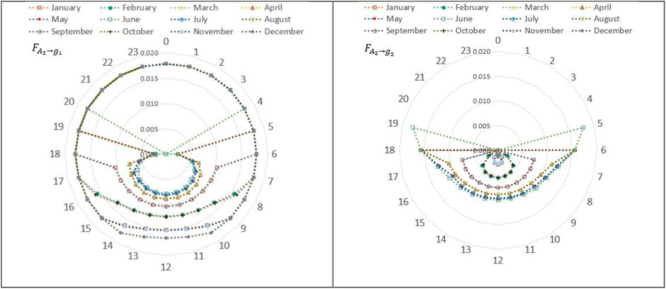
FIGURE 15. Radar chart representing $F_{A_2\to g_1}$ and $F_{A_2\to g_2}$ for the 21st of every month.

Since the values of $F_{A_2\to g_1}$ and $F_{A_2\to g_2}$ are complementary and dependent on shaded and unshaded profiles, increasing the shadow length leads to an increase in $F_{A_2\to g_1}$ and a decrease in $F_{A_2\to g_2}$, and vice versa. The symmetry of the two profiles can be observed in Figure 15.

The view factor between the surface of the second row and surrounding ground; ${\mathit{F}}_{{\mathit{A}}_2\to \mathit{g}}$

The subscription g refers to the ground surrounding the second, not including the space separating the rows ($g_1+g_2$) and assumed to be unshaded. The value of $F_{A_2\to g}$ is obtained by applying the summation rule as follows:

$\begin{array}{l}{F}_{A_2\to g}=1-\left(F_{A_2\to \left(g_1+g_2\right)}+F_{A_2\to sky}+F_{A_2\to A_{1r}}\right)\\ F_{A_2\to g}=1-\left(0.0179+0.9454+0.0244\right)=\mathrm{0.0123.}\end{array}(29)$

3.6.2 View Factor of the Rear Surface of the First Row $F_{A_{1r}}$

In actuality, the rear surface of the first row is a reverse image of the second row and deal in the same manner as the second row.

The view factor between the rear surface of the first row and space-separating rows; ${\mathit{F}}_{{\mathit{A}}_{1\mathit{r}}\to (\mathit{g}1+{\mathit{g}}_2)}$

The view factor $F_{A_{1r}\to (g1+g_2)}$ is a constant value dependent only on design parameters. It is determined from Eq. 18.

$F_{A_{1r}\to (g1+g_2)}=\mathrm{0.9176.}(30)$

The view factor between the rear surface of the first row and the shaded zone; ${\mathit{F}}_{{\mathit{A}}_{1\mathit{r}}\to {\mathit{g}}_1}$

The view factor between the rear surface of the first row and the shaded zone g₁ is calculated by applying Eq. 15.

The view factor between the surface of the second row and the sunny zone; ${\mathit{F}}_{{\mathit{A}}_{1\mathit{r}}\to {\mathit{g}}_2}$

The view factor between the rear surface of the first row and the unshaded zone g₂ is obtained by using the view factor algebra summation rule Eq. 2 by subtracting the value of $F_{A_{1r}\to g_1}$ from the view factor of the total space separating the rows $F_{A_{1r}\to (g1+g_2)}$.

$F_{A_{1r}\to g_2}=F_{A_{1r}\to \left(g_1+g_2\right)}-F_{A_{1r}\to g_1}.(31)$

The dynamic values of $F_{A_{1r}\to g_1}$ and $F_{A_{1r}\to g_2}$ are depicted in the form of radar charts in Figure 16 for the 21st of every month.

FIGURE 16

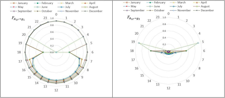
FIGURE 16. Hourly values of $F_{A_{1r}\to g_1}$ and $F_{A_{1r}\to g_2}$ for the 21st of every month.

The value of $F_{A_{1r}\to g_1}$ is high at low tilt angles, influenced largely by the width of the shaded zone Z₁. The relationship is clearly demonstrated by the similarities in Figure 16 in that the value of $F_{A_{1r}\to g_1}$ goes up with an increase in width of the shaded zone Z₁ and vice versa.

The view factor between the rear surface of the first row and surrounding ground; ${\mathit{F}}_{{\mathit{A}}_{1\mathit{r}}\to \mathit{g}}$

The view factor $F_{A_{1r}\to g}$ is treated in the same way as with sky view factor of the second row $F_{A_2\to sky}$ using the superposition rule. The rear surface of the first row sees the surrounding ground in the same manner as the first row sees the sky ($F_{A_1\to s}$), less blocking takes place due to the presence of the second row ($F_{A_2\to A_{1r}}$) and the space separating the rows, giving the following equation:

$\begin{array}{l}{F}_{A_{1r}\to g}=\frac{1+cos\beta }{2}-\left(F_{A_{1r}\to \left(g_1+g_2\right)}+F_{A_2\to A_{1r}}\right)\\ F_{A_{1r}\to g}=0.9698-\left(0.9176+0.0244\right)=\mathrm{0.0278.}\end{array}(32)$

This value represents what the row sees from the ground surrounding the row, assumed to be unshaded.

The view factor between the rear surface of the first row and sky; ${\mathit{F}}_{{\mathit{A}}_{1\mathit{r}}\to \mathit{s}}$

The view factor $F_{A_{1r}\to s}$ is a constant value and it is dependent only on the design parameters and treated in the same manner as $F_{A_2\to g}$ using the summation rule, giving the following equation:

$\begin{array}{l}{F}_{A_{1r}\to s}=1-\left(F_{A_1\to g}+F_{A_1\to \left(g_1+g_2\right)}+F_{A_2\to A_{1r}}\right)\\ F_{A_{1r}\to s}=1-(0.0278+0.9176+0.0244=\mathrm{0.0302.}\end{array}(33)$

4 Solar Irradiance Calculation

The main objective of this research is the estimation of solar irradiance incident on the second and subsequent rows of a horizontal plane fixed-mode solar PV fields. The classical approach for calculating solar irradiance incidents on a single-tilted surface is well documented in solar energy engineering textbooks (Nassar, 2006; Duffie and Beckman, 2013). Calculating global solar irradiance ($I_t$) incident on an inclined surface requires global horizontal ($I_h$) data. $I_h$ has two components direct beam ($I_{bh}$) and sky diffuse ($I_{dh}$) irradiance. The global horizontal solar irradiance ($I_h$) is given by the following equation:

$I_h=I_{bh}+I_{dh}.(34)$

$I_h$ and $I_{dh}$ can be measured and are obtainable from databases on solar energy websites. The horizontal solar radiation data used in this research is 13-years hourly time series obtained from Solargis (https://solargis.com/). Figures 17, 18 present the diffuse and beam solar irradiance as function of time for Tripoli and Ankara.

FIGURE 17

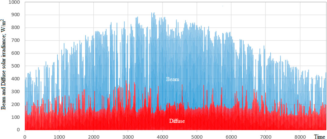
FIGURE 17. Hourly horizontal beam and diffuse solar irradiance for Tripoli ($32.815°N, 13.439°E$).

FIGURE 18

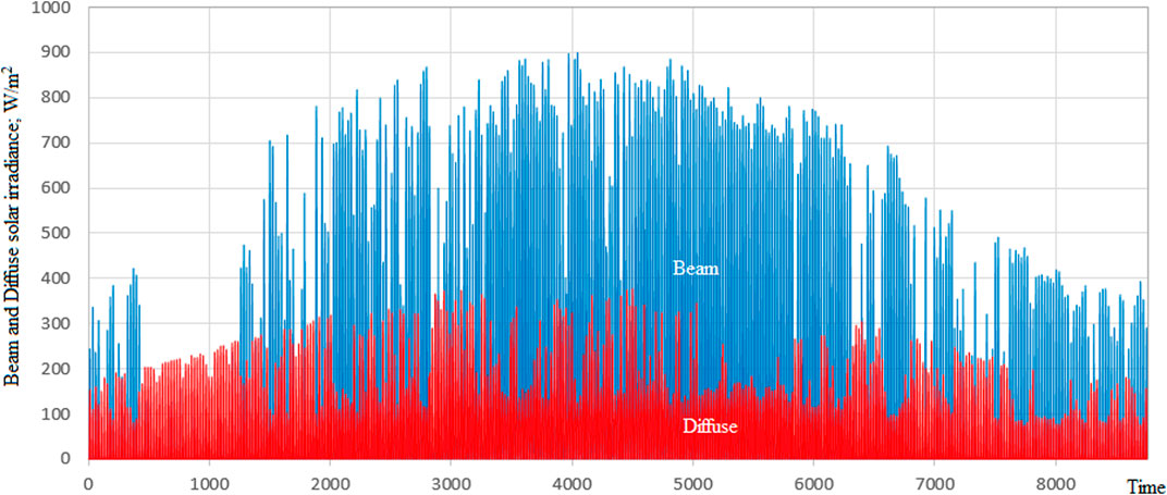
FIGURE 18. Hourly horizontal beam and diffuse solar irradiance for Ankara ($40.05°N, 32.867°E$).

Transposition models are used to transpose global horizontal solar irradiance to tilted irradiance, giving global irradiance for tilted surface ($I_t$) at a tilt angle (β) from the horizontal as follows:

$I_t=I_{bh}{R}_b+I_{dh}{F}_{A_1\to S}+I_h {\rho }_g F_{A_1\to g},(35)$

where ${\rho }_g$ is the albedo radiation factor, generally assumed to be 0.2. The transposition factor ($R_b$) is given as a function of geometrical parameters of inclined surface and position of the Sun:

$R_b=max\left(0,\frac{cos{\theta }_i}{cos{\theta }_z}\right),(36)$

where ${\theta }_i$ and ${\theta }_z$ are solar incidence and zenith angles, respectively.

Similarly, $F_{A_1\to g}$ is the view factor between a single surface and ground-reflected solar irradiance. It is given by the following equation:

$F_{A_1\to g}=\frac{1-\cos \beta }{2}.(37)$

The diffuse irradiance is due to the scattering of solar radiation by different elements of the atmosphere. Therefore, it has a naturally non-uniform distribution throughout the sky. However, some models consider diffuse irradiance uniform or isotropic, known as isotropic models. Other models are based on the assumption that all the diffuse irradiance can be represented by two parts the isotropic and the circumsolar. Other models try to depict the scattering process by adding the diffuse irradiance coming from the circumsolar region and the horizon band to the isotropic background. The last two approaches are known as anisotropic models. Therefore, the models used to estimate ($I_{dt}$) or the transposition models could be divided into two groups as follows: isotropic and anisotropic (Nassar et al., 2020).

The most popular model used in the isotropic family is the Liu-Jordan Model (Liu and Jordan, 1961), where the sky view factor ($F_{A_1\to S}$) is given by the following equation:

$F_{A_1\to S}=\frac{\left(1+\cos \beta \right)}{2}.(38)$

An example of the anisotropic approach is the Hay–Davies Model (Hay and Davies, 1978) expressed as follows:

$F_{A_1\to S}=F_{Hay}{R}_b+\left(1-F_{Hay}\right)\left(\frac{1+cos\beta }{2}\right),(39)$

where $F_{Hay}=I_{bh}/I_{sc}$ is the modified Hay’s factor.

The irradiance components associated with a solar PV field are more complex than those of a single surface. The classical approach accounts for beam (I_bh) irradiance, diffuse (I_dh) irradiance, and reflected irradiance from the ground (I_r) and from the rear of the front row. In reality, there are additional components that ought to be considered in a solar PV field, namely the view factors between the second and proceeding rows with the sky dome and with the ground surface.

Alsadi and Nassar (2017b) presented a mathematical form for an isotropic sky model as follows:

$I_{f,iso=}\{\begin{array}{l}{I}_{bh}{\forall }_{A_2}{R}_{b{A}_2}+\\ I_{dh}{F}_{A_2\to S}+\\ \left[\left(I_{bh}+I_{dh}\right)\left(\frac{Z_2}{W}{F}_{A_2\to g_2}+F_{A_2\to g}\right)+I_{dh}\frac{Z_1}{W}{F}_{A_2\to g_1}\right]{\rho }_g+\\ +\left[\begin{array}{l}{\rho }_g\left[\left(I_{bh}+I_{dh}\right)\left(\frac{Z_2}{W}{F}_{A_{1r}\to g_2}+F_{A_{1r}\to g}\right)+I_{dh}\frac{Z_1}{W}{F}_{A_{1r}\to g_1}\right]+\\ +\left[I_{bh}{\forall }_{A_{1r}}{R}_{b{A}_{1r}}+I_{dh}{F}_{A_{1r}\to S}\right]\end{array}\right]{\rho }_{A_{1r}}{F}_{A_2\to A_{1r}}\end{array}(40)$

where ${\forall }_{A_2}$ is the ratio of the unshaded area to the total surface area.

The Hay–Davies model may be rearrangement according to the definition of the problem stated graphically in Figure 1 as follows:

$I_{f,aniso=}\{\begin{array}{l}{I}_{bh}{\forall }_{A_2}{R}_{b{A}_2}\\ +I_{dh}\left[\left(F_{Hay}{R}_{b{A}_2}\right)+\left(1-F_{Hay}\right)F_{A_2\to s}\right]\\ \left[\left(I_{bh}+I_{dh}\right)\left(\frac{Z_2}{W}{F}_{A_2\to g_2}+F_{A_2\to g}\right)+I_{dh}\frac{Z_1}{W}{F}_{A_2\to g_1}\right]{\rho }_g+\\ +\left[\begin{array}{l}{\rho }_g\left[\left(I_{bh}+I_{dh}\right)\left(\frac{Z_2}{W}{F}_{A_2\to g_2}+F_{A_2\to g}\right)+I_{dh}\frac{Z_1}{W}{F}_{A_{1r}\to g_1}\right]+\\ +I_{dh}\left[\left(F_{Hay}{R}_{b{A}_{1r}}\right)+\left(1-F_{Hay}\right)F_{A_{1r}\to s}\right]\end{array}\right]{\rho }_{A_{1r}}{F}_{A_2\to A_{1r}}\end{array}(41)$

To illustrate the impact of view factors on the estimation of solar irradiance incident on a solar harvester, we will investigate the performance of three different solar PV systems; a solar PV field, a rooftop solar PV system, and a single PV surface. For the purpose of this comparison, the aspect ratio $\frac{L}{W}$ for the solar PV field and rooftop solar PV installation is assumed 33.33 and 5, respectively. The analysis was carried for two locations, Tripoli ($\varnothing ={32.8}^{°}N$) and Ankara ($\varnothing =40°N$).

First, we will consider the case where the solar PV field rows are shadow-free (${\forall }_{A_2}=1$). The obtained results are tabulated in Table 2.

TABLE 2

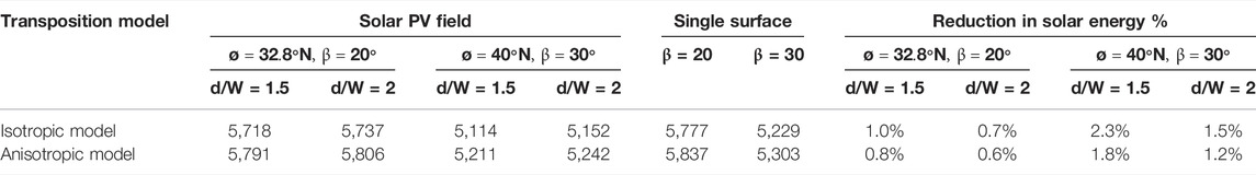
TABLE 2. Daily solar radiation [W/m²/day] incident on the solar PV field and the single surface, no shading conditions.$\left({\forall }_{A_2}=1\right)$

The analysis results (Table 2) clearly show reduced solar energy yield for the solar PV field compared to the single surface. The results also show the impact of location on solar energy yield, where energy reduction at high latitudes is more than twice than that at middle latitudes. The impact of location is directly related to the row’s tilt angle, optimized to receive maximum solar energy, and the distance separating the rows, which is governed by economic considerations.

Next, we will consider the effect of shadow falling on the solar PV field rows (${\forall }_{A_2}=0$). The hourly solar radiation incident on the surface of the second and subsequent rows can be calculated using Eq. 38 for the isotropic model and Eq. 39 for the anisotropic model. The obtained results are tabulated in Table 3.

TABLE 3

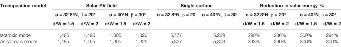
TABLE 3. Daily solar radiation [W/m²/day] incident on the solar PV field and the single surface, shading conditions (${\forall }_{A_2}=0$).

A side note of the results in Table 3 is the similarity of isotropic and anisotropic model results. This is a direct consequence of eliminating the beam component of solar radiation. The influence of the view factors, especially the sky view factor, become more pronounced and the reduction in solar radiation becomes dramatic (exceeding 300% at high latitudes).

An investigation for overcast sky leads to more specific results as tabulated in Table 4.

TABLE 4

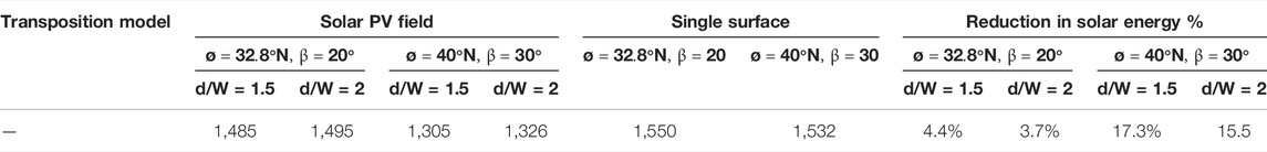
TABLE 4. Daily solar radiation [W/m²/day] incident on the solar PV field and the single surface, under overcast sky conditions.

Again, the performance of isotropic and anisotropic models is the same in the absence of beam radiation.

Table 4 shows that reduction in solar energy in the solar PV field is significantly higher compared to single surface under overcast sky conditions (exceeding 4 and 17% at mid and high latitudes, respectively). This is explained by the increase in the diffuse component of solar radiation, which in turn is a function of the sky view factor.

The other aspect of this investigation looks into the second type of solar PV installations, namely rooftop solar PV. The obtained results are tabulated in Table 5.

TABLE 5

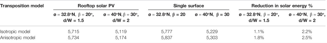
TABLE 5. Daily solar radiation [W/m2/day] incident on rooftop solar PV installation ($\frac{L}{W}=5$).

Table 5 shows that the solar energy incident on a rooftop solar PV installation is approximately 2% lower than that of a single surface.

5 Conclusion

This research used 3-D numerical analysis to calculate the view factors of a horizontal plane fixed-mode solar PV field. However, it can equally be applied to all types of solar fields, including rooftops and building façades. It only requires defining the view factors between the PV panels and the environment. The influence of the design parameters, location, and time are analyzed. The present study shows that the tilt angle has a higher weighting compared to other design parameters.

The key finding of this research is improved accuracy of estimation of solar PV field potential by introducing a model for estimating reduction in solar irradiance incident on the second and subsequent rows relative to the first row of a solar field. The obtained results showed that reduction in solar irradiance is higher at high latitudes, reaching 2.3%. In addition, the reduction in solar irradiance is high under overcast sky conditions, reaching 17% at high latitudes and up to 5% in the North African region, and 300% reduction in solar radiation for shaded zones. It is highly advisable that shading in solar fields can be avoided where possible measures might be affected, such as reducing the tilt angle and/or increasing the distance separating the rows. The latter measure has some economic implications which need to be considered.

The present research is also tested the validity of the CSM for wide ranges of distance separating rows and length aspect ratios, the obtained results show that, the CSM shows good agreements in both sky and the ground view factor in the range of the length aspect ratio greater than one, but it fails in the rear side view factor in the design ranges of PV solar fields, where the error rate was found about 11%, this result is important in the case of bifacial PV solar systems.

Data Availability Statement

The original contributions presented in the study are included in the article/Supplementary Material, further inquiries can be directed to the corresponding author.

Author Contributions

YN: conceptualization; methodology; programming; and writing—original draft. HE-K: formal analysis and writing—reviewing and editing. SB: programming and writing and editing. SA: data collection and formal analysis. NA: revising the manuscript; formal analysis.

Conflict of Interest

The authors declare that the research was conducted in the absence of any commercial or financial relationships that could be construed as a potential conflict of interest.

Publisher’s Note

All claims expressed in this article are solely those of the authors and do not necessarily represent those of their affiliated organizations, or those of the publisher, the editors, and the reviewers. Any product that may be evaluated in this article, or claim that may be made by its manufacturer, is not guaranteed or endorsed by the publisher.

References

Agha, K. R., and Sbita, M. N. (2000). On the Sizing Parameters for Stand-Alone Solar-Energy Systems. Appl. Energ. 65, 73–84. doi:10.1016/s0306-2619(99)00093-8

CrossRef Full Text | Google Scholar

Alam, M., Gul, M. S., and Muneer, T. (2019). Radiation View Factor for Building Applications: Comparison of Computation Environments. Energies 12, 3826. doi:10.3390/en12203826

CrossRef Full Text | Google Scholar

Alsadi, S. Y., and Nassar, Y. F. (2017). A Numerical Simulation of a Stationary Solar Field Augmented by Plane Reflectors: Optimum Design Parameters. Sgre 08, 221–239. doi:10.4236/sgre.2017.87015

CrossRef Full Text | Google Scholar

Alsadi, S. Y., and Nassar, Y. F. (2017). Estimation of Solar Irradiance on Solar Fields: An Analytical Approach and Experimental Results. IEEE Trans. Sustain. Energ. 8 (4), 1601–1608. doi:10.1109/TSTE.2017.2697913

CrossRef Full Text | Google Scholar

Alsadi, S. Y., and Nassar, Y. F. (2019). A General Expression for the Shadow Geometry for Fixed Mode Horizontal, Step-like Structure and Inclined Solar fields. Solar Energy 181, 53–69. doi:10.1016/j.solener.2019.01.090

CrossRef Full Text | Google Scholar

Alsadi, S., Nassar, Y., and Ali, K. (2016). General Polynomial for Optimizing the Tilt Angle of Flat Solar Energy Harvesters Based on ASHRAE clear Sky Model in Mid and High Latitudes. Energy and Power 6 (2), 29–38. doi:10.5923/j.ep.20160602.0

CrossRef Full Text | Google Scholar

Appelbaum, J., and Aronescu, A. (2016). View Factors of Photovoltaic Collectors on Roof Tops. J. Renew. Sust. Energ. 8, 025302. doi:10.1063/1.4943122

CrossRef Full Text | Google Scholar

Appelbaum, J. (2018). The Role of View Factors in Solar Photovoltaic fields. Renew. Sust. Energ. Rev. 81, 161–171. doi:10.1016/j.rser.2017.07.026

CrossRef Full Text | Google Scholar

Arias-Rosales, A., and LeDuc, P. R. (2020). Comparing View Factor Modeling Frameworks for the Estimation of Incident Solar Energy. Appl. Energ. 277, 115510. doi:10.1016/j.apenergy.2020.115510

CrossRef Full Text | Google Scholar

Baehr, H. D., and Karl, S. (2011). Heat and Mass Transfer. 3rd ed. Berlin, Heidelberg: Springer, 588.

Google Scholar

Duffie, J., and Beckman, W. (2013). Solar Engineering of Thermal Processes. 4th ed. New York: Wiley.

Google Scholar

Groumpos, P. P., and Khouzam, K. (1987). A Generic Approach to the Shadow Effect of Large Solar Power Systems. Solar Cells 22 (1), 29–46. doi:10.1016/0379-6787(87)90068-8

CrossRef Full Text | Google Scholar

Gupta, M. K., Bumtariya, K. J., Shukla, H., Patel, P., and Khan, Z. (2017). Methods for Evaluation of Radiation View Factor: A Review. Mater. Today Proc. 4, 1236–1243. doi:10.1016/j.matpr.2017.01.143

CrossRef Full Text | Google Scholar

Hay, J., and Davies, J. (1978). “Calculation of the Solar Radiation Incident on an Inclined Surface,” in Proceedings of the First Canadian Solar Radiation Data Workshop, April 17-19, 1978: Toronto, Ontario, Canada (Ottawa: Minister of Supply and Services Canada), 59–72.

Google Scholar

Howell, J. R. (2016). A Catalog of Radiation Heat Transfer Configuration Factors. Available at: http://www.thermalradiation.net/indexCat.html (Accessed date January 14, 2022).

Google Scholar

Liu, B., and Jordan, R. (1961). Daily Insolation on Surfaces Tilted towards Equator. ASHRAE Trans. 67, 526–541. Available at: https://www.osti.gov/scitech/biblio/5047843.

Google Scholar

Mubarak, R., Hofmann, M., Riechelmann, S., and Seckmeyer, G. (2017). Comparison of Modelled and Measured Tilted Solar Irradiance for Photovoltaic Applications. Energies 10, 1688. doi:10.3390/en10111688

CrossRef Full Text | Google Scholar

Nassar, Y. F., and Alsadi, S. Y. (2016). View Factors of Flat Solar Collectors Array in Flat, Inclined, and Step-like Solar Fields. ASME. J. Sol. Energ. Eng. 138 (6), 061005. doi:10.1115/1.4034549

CrossRef Full Text | Google Scholar

Nassar, Y. F., and Alsadi, S. Y. (2019). Assessment of Solar Energy Potential in Gaza Strip-Palestine. Sustainable Energ. Tech. Assessments 31, 318–328. doi:10.1016/j.seta.2018.12.010

CrossRef Full Text | Google Scholar

Nassar, Y. F., Hadi, H. H., and Salem, A. A. (2008). Time Tracking of the Shadow in the Solar Fields. J. Sebha Univ. 7 (2), 59–73.

Google Scholar

Nassar, Y. F., Hafez, A. A., and Alsadi, S. Y. (2020). Multi-Factorial Comparison for 24 Distinct Transposition Models for Inclined Surface Solar Irradiance Computation in the State of Palestine: A Case Study. Front. Energ. Res. 7, 163. doi:10.3389/fenrg.2019.00163

CrossRef Full Text | Google Scholar

Nassar, Y. (2005). Simulation of Solar Tracking Systems. Energ. Life J. 21, 81–90.

Google Scholar

Nassar, Y. F. (2006). Solar Energy Engineering-Active Applications. Libya: Sebha University.

Google Scholar

Nassar, Y. F. (2020). Analytical-Numerical Computation of View Factor for Several Arrangements of Two Rectangular Surfaces with Non-common Edge. Int. J. Heat mass transfer 159, 120130. doi:10.1016/j.ijheatmasstransfer.2020.120130

CrossRef Full Text | Google Scholar

Pomax, M. K. (2011). Gaussian Quadrature Weights and Abscissae. Available at: https://pomax.github.io/bezierinfo/legendre-gauss.html (Accessed date March 31, 2022).

Google Scholar

Refschneider, W. E. (1967). Radition Geometry in Measurement and Interpretation of Radiation Balance. Agric. Meteorol. 4, 255–265.

Google Scholar

Rehman, N. U., and Uzair, M. (2017). The Proper Interpretation of Analytical Sky View Factors for Isotropic Diffuse Solar Irradiance on Tilted Planes. J. Renew. Sust. Energ. 9, 053702. doi:10.1063/1.4993069

CrossRef Full Text | Google Scholar

Seme, S., Sredenšek, K., Štumberger, B., and Hadžiselimović, M. (2019). Analysis of the Performance of Photovoltaic Systems in Slovenia. Solar Energy 180 (1), 550–558. doi:10.1016/j.solener.2019.01.062

CrossRef Full Text | Google Scholar

Vokony, I., Hartmann, B., Talamon, A., and Viktor, R. (2018). On Selecting Optimum Tilt Angle for Solar Photovoltaic Farms. Int. J. Renew. Energ. Res. 8 (No.4), 1926–1935. doi:10.20508/ijrer.v8i4.8285.g7501

CrossRef Full Text | Google Scholar

Vujičić, M., Lavery, N., and Brown, S. (2016). Numerical Sensitivity and View Factor Calculation Using the Monte Carlo Method. Proc. Imeche Part. C: J. Mech. Eng. Sci. 220, 697–702. doi:10.1243/09544062JMES139

CrossRef Full Text | Google Scholar

Weisstein, E. W. (2013). Legendre-Gauss Quadrature, MathWorld--A Wolfram Web. Available at: https://mathworld.wolfram.com/Legendre-GaussQuadrature.html (Accessed date April 19, 2022).

Google Scholar

APPENDIX I

Two rectangles with one common edge and included angle Φ (Howell, 2016).

$A=\frac{a}{c}, B=\frac{b}{c}, C=A^2+B^2-2ABcos\varnothing , \text{and} D={\left(1+A^{2}si{n}^2\varnothing \right)}^{1/2}$

$\begin{array}{l}{F}_{1-2}=-\frac{\sin 2\Phi }{4\pi B}\left[AB\sin \Phi +\left(\frac{\pi }{2}-\Phi \right)\left(A^2+B^2\right)+B^2{\tan }^{-1}\left(\frac{A-B\cos \Phi }{B\sin \Phi }\right)+A^2{\tan }^{-1}\left(\frac{B-A\cos \Phi }{A\sin \Phi }\right)\right]\\ +\frac{{\sin }^2\Phi }{4\pi B}\left\{\left(\frac{2}{{\sin }^2\Phi }-1\right)\ln \left[\frac{\left(1+A^2\right)\left(1+B^2\right)}{1+C}\right]+B^2\ln \left[\frac{B^2(1+C)}{\left(1+B^2\right)C}\right]+A^2\ln \left[\frac{A^2{(1+A^2)}^{\cos 2\Phi }}{C{\left(1+C\right)}^{\cos 2\Phi }}\right]\right\}\\ +\frac{1}{\pi }{\tan }^{-1}\left(\frac{1}{B}\right)+\frac{A}{\pi B}{\tan }^{-1}\left(\frac{1}{A}\right)-\frac{\sqrt{C}}{\pi B}{\tan }^{-1}\left(\frac{1}{\sqrt{C}}\right)\\ +\frac{\sin \Phi \sin 2\Phi }{2\pi B}AD\left[{\tan }^{-1}\left(\frac{A\cos \Phi }{D}\right)+{\tan }^{-1}\left(\frac{B-A\cos \Phi }{D}\right)\right]\\ +\frac{\cos \Phi }{\pi B}{\displaystyle {\int }_0^B\sqrt{1+{\xi }^2{\sin }^2\Phi }}\left[{\tan }^{-1}\left(\frac{\xi \cos \Phi }{\sqrt{1+{\xi }^2{\sin }^2\Phi }}\right)+{\tan }^{-1}\left(\frac{A-\xi \cos \Phi }{\sqrt{1+{\xi }^2{\sin }^2\Phi }}\right)\right]d\xi \end{array}$

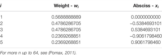
The last term remains unsolved. In this research, this term is solved numerically by means of Gaussian quadrature five-point rule. The weights ($w_i$) and abscissae ($x_i$) for use in performing Legendre–Gauss quadrature integral approximation, which tries to solve the following function (Weisstein, 2013):

$\underset{a}{\overset{b}{{\displaystyle \int }}}f\left(x\right)dx\cong {\displaystyle \sum }_{i=1}^n{w}_{i}f\left(x_i\right)$

$\underset{a}{\overset{b}{{\displaystyle \int }}}f\left(x\right)dx\cong \frac{b-a}{2}\underset{-1}{\overset{1}{{\displaystyle \int }}}f\left(\frac{b-a}{2}{x}_i+\frac{b+a}{2}\right)\cong \frac{b-a}{2}{\displaystyle \sum }_{i=1}^n{w}_i f\left(\frac{b-a}{2}{x}_i+\frac{b+a}{2}\right)$

Weights and Abscissae Table for n = 5 (Pomax, 2011).

Nomenclature

A Surface area; m²

$F_{i-j}$ View factor between surfaces i and j

d Distance separating rows of the solar field; m

W Width of row of the solar field; m

L Length of the row of the solar field; m Latitude angle

Z₁ Width of the shadow zone; m

Z₂ Width of the unshaded zone; m

$I_h$ Global horizontal solar irradiance; W/m²

$I_{bh}$ Beam horizontal solar irradiance; W/m²

$I_{dh}$ Sky diffuse solar irradiance on the horizontal surface; W/m²

$I_t$ Global tilted surface solar irradiance; W/m²

$I_f$ Global solar irradiance in the solar field; W/m²

β Surface tilt angle

$\psi$ Surface azimuth angle

$ø$ Solar azimuth angle

α Solar altitude angle

L Length of the row of the solar field; m Latitude angle

θi Solar incident angle

θz Solar zenith angle

ρ Reflectivity

∀ Shaded to total surface area ratio

Subscriptions:

g Ground

s Sky

g₁ ground shaded zone

g₂ ground unshaded zone

A₁ First row surface

A₂ Second row surface

A_1r rear surface of the first row

iso Isotropic sky analysis

aniso Anisotropic sky analysis