Reliability Synthesis and Prediction for Complex Electromechanical System: A Case Study

Introduction

Complex electromechanical systems (CEMSs) have been used in industry, civil machinery, aerospace, and so on (Mi et al., 2016; Wang et al., 2022). Reliability synthesis and prediction of CEMSs have long been critical issues within the field of reliability engineering. CEMSs are usually composed of optics, machinery, and electricity (Tang et al., 2021). Some CEMSs have very complex structures, some have huge volumes, some have long service life, and some are expensive (Han et al., 2021). Thus, reliability synthesis and prediction of CEMSs only relying on life testing are limited by multiple factors such as test scheme, test site, test time, test cost, and test conditions. However, at the stage of the project demonstration and initial design of CEMSs, reliability synthesis and prediction of CEMSs are necessary (Fuqiu et al., 2020). Therefore, it challenges the realization of reliability synthesis and prediction of CEMSs.

Since Buehler proposed a reliability synthesis method for a series system with two binomial components (Buehler, 1957), scholars from classical, Bayes, and fiducial schools have conducted a lot of research on reliability synthesis and prediction of systems. The classical school put forward the maximum likelihood estimation (MLE) method, modified maximum likelihood estimation (MML) method, sequential reduction (SR) method, combined MML and SR method (CMSR), and so on (Yu et al., 2013). The MLE method is only applicable to large sample tests, and the failure distribution is an unbounded symmetric normal distribution. The MML method is only applicable to binomial (pass–fail) component systems (Fo and Xiong, 2009). The disadvantage of the SR method is that successive compression of test data leads to information loss, resulting in large estimation variance and a more conservative confidence limit of system reliability (Zhu and J Sh, 1990). The algorithm of the CMSR method is complex, and it is not suitable for the system with zero failure number of unit test data. The Bayes method only solves the reliability interval estimation of binomial or exponential approximation for complex systems (Guo and Wilson, 2013). The fiducial method has been proved unsuitable for system reliability evaluation (Zhou and Weng, 1990). Therefore, it is difficult to use the abovementioned methods to synthesize and predict the CEMSs’ reliability, and reliability synthesis and prediction of CEMSs are still problems in reliability engineering (Peng et al., 2013). Although the Monte Carlo method can easily deal with the reliability synthesis problem of systems with different unit distributions (Yeh et al., 2010), the simple Monte Carlo method, bootstrap method, double Monte Carlo method, and asymptotic method introduced in many studies can only solve the lower confidence limit of system reliability, and the interval estimation problem of system life distribution types and parameters are unsolved (Meng and Wen-Tao, 2021). Despite decades of research, there is still no general method to realize the reliability synthesis and prediction of CEMSs (Kovacs et al., 2019).

It is well known that a CEMS is composed of several units (subsystems), and the system reliability depends on the reliability of its constituent units (subsystems) (Negi and Singh, 2015), (Liu et al., 2015). When the constituent units’ life of CEMS follows different distributions, it is difficult to synthesize and predict the CEMS reliability from units’ reliability data information (Weiyan et al., 2009). Hence, some scholars have conducted a lot of correlational research. For example, Guo et al. (2014) analyzed some theories and methods for system reliability synthesis, and the new idea was proposed for the problem aiming at specific engineering backgrounds. Considering that some CEMSs contain outsourced components, Sun et al. (2018) computed system reliability and component importance measures. According to the equal-principle first and second moment of reliability, Yu et al. (2013) investigated Bayes reliability confidence limit for a series-parallel system consisting of different distribution units. Graves and Hamada (2016) evaluated the likelihood for simultaneous failure time data when monitoring was stopped. In view of the lack of reliability data information of CEMSs, Wilson et al. (2006) and Yuan et al. (2019) discussed how to make full use of limited reliability data information of CMESs to synthesize and predict system reliability. Although scholars have discussed the reliability synthesis and prediction of CEMS from many aspects, there are still challenges by many factors such as difficulty in establishing a reliability model for CMES, lack of reliability data information, high test cost, and so on. It is necessary to be studied further.

In order to solve the above problems and realize the reliability synthesis and prediction of CEMS, a numerical analysis method based on the computer simulation and the Monte Carlo (MC) method is proposed in this article. The remainder of this article is organized as follows: In Section 2, we propose a method to obtain the life simulation values for the constituent units of CEMS when the life distribution types and distribution parameters of constituent units are known. In Section 3, we take a method to obtain the system life simulation value from the units’ life simulation values. One system life simulation value represents a reliability test of CEMS. Computer simulation can be realized instead of life test when there are enough system life simulation values. In Section 4, we carry out the initial selection of CMES life distribution types and goodness-of-fit test. In Section 5, a case study of a CMES is presented to demonstrate the effectiveness of our proposed method. Finally, conclusions are made in Section 6.

Life Simulation Values for the Constituent Units of Complex Electromechanical Systems

It is assumed that a CEMS is composed of n different life distribution units, and the life distribution and the appropriate parameters of each constituent unit are known. The life simulation values for n units are generated using the random variable simulation conversion equation and through Monte Carlo simulation (Yoshida and Akiyama, 2011; Wang et al., 2012; Zhang et al., 2014). According to the common distributions in engineering, such as the exponential distribution, Weibull distribution, normal distribution, logarithmic normal distribution, extreme value distribution, Gamma distribution etc., the respective random variable simulation conversion equations $g\left({\vartheta }_i\right)$ are deduced and listed in Table 1. If a unit is subject to any other distribution, its random variable simulation conversion equation can be solved similarly using the inverse function method.

TABLE 1

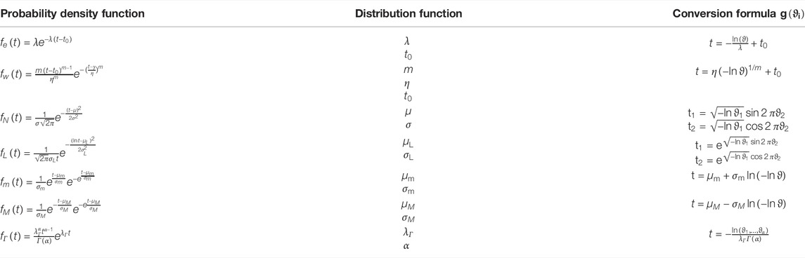
TABLE 1. Conversion formulas of different distributions.

In order to ensure that all units are independent of each other, the pseudo-random number is computer-generated for each unit and subject to 0-1uniform distribution.

${\mathit{\vartheta }}_i=\mathrm{R}\mathrm{N}\mathrm{D}\left(1\right)i=\mathrm{1,2},\cdots ,n.$

According to the life distribution and parameters of each constituent unit, the life simulation value $t_i$ for the corresponding unit can be obtained through logical operation.

$t_i=g\left({\mathit{\vartheta }}_i\right)i=\mathrm{1,2},\cdots ,n.$

In this way, a set of life simulation values of n units can be obtained, and the first simulation values are completed. The m groups of life simulation values are obtained after m cycles.

Life Simulation Values for the Complex Electromechanical Systems

For the CEMS composed of n units, the life simulation value for each unit can be obtained through each simulation, and they are denoted by $t_{j1},t_{j2},\cdots ,t_{jn}$. According to the reliability logical relationship between the CEMS and each component unit, the life simulation values for the CMES are obtained on the minimal path set method (Cancela et al., 2013; Schallert, 2014).

$\mathit{S}={\displaystyle \underset{h=1}{\overset{q}{\cup }}{\mathit{S}}_h}={\displaystyle \underset{h=1}{\overset{q}{\cup }}\left[{\displaystyle \underset{x_i,x_j,\cdots \in S_h}{\cap }\left(x_i,x_j,\cdots \right)}\right]},(1)$

where S denotes the CEMS, q denotes the number of the minimum path sets in the CEMS, $h=\mathrm{1,2},\cdots ,q$, and $S_h=\left(x_i,x_j,\cdots \right)$, $x_i,x_j$… is all the units in a minimum path set.

Therefore, the life simulation value $t_S$ for a CEMS can be obtained through logical operation after each simulation.

$t_S=\underset{1<h<q}{\mathit{max}}\left(t_{S_h}\right)=\underset{1<h<q}{\mathit{max}}\left[\underset{t_i,t_j\dots \in S_h}{\mathit{min}}\left(t_i,t_j,\dots \right)\right],(2)$

where $t_S$ is the life simulation value for the CEMS, $t_i,t_j$… is the life simulation value for each unit in the minimum path set, and $t_{S_h}$ is the life simulation value for the hth minimum path set.

The minimal path sets of the typical system are shown in Figure 1, and the system has four minimum path sets: $\left(x_1,x_5,x_4\right)$, $\left(x_2,x_5,x_3\right)$. The life simulation values for the system are obtained by the following equation (Hong-Bo and Guo, 2009):

$t_S=\max [\min \left(t_1,t_2\right),\min \left(t_3,t_4\right),\min \left(t_1,t_5,t_4\right),\min \left(t_3,t_5,t_2\right)].(3)$

FIGURE 1

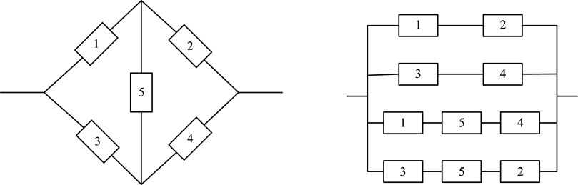
FIGURE 1. Minimal path sets of typical system.

In general, the CEMS is usually considered to be composed of several simple serial or parallel subsystems, and the following equations are established:

$t_{Sk}=\underset{t_i,t_j\dots \in S_k}{\mathit{min}}\left(t_i,t_j,\dots \right),(4)$

$t_{Sl}=\underset{t_i,t_j\dots \in S_l}{\max }\left(t_i,t_j,\dots \right),(5)$

where $t_{Sk}$ is the life simulation value for the serial subsystem and $t_{Sl}$ is the life simulation value for the parallel subsystem.

For any CEMS, the simulation value array $T\left(r\times n\right)$ for the units can be obtained by carrying out $r$ simulations over n component units.

$T\left(r\times n\right)=\left|\begin{array}{l}{t}_{11},t_{21},\cdots ,t_{n1}\\ t_{12},t_{22},\cdots ,t_{n2}\\ ⋮\\ t_{1r},t_{2r},\cdots ,t_{nr}\end{array}\right|.(6)$

Each simulation can yield a set of life simulation values for the units, and one life simulation value for the system can be obtained by Eq. 2. If r simulations are performed, r life simulation values can be obtained, namely, $t_{S1},t_{S2},\mathrm{...},t_{Sr}$, and t_Sr is equivalent to the full life test over r CEMSs. If r is large enough, the life distribution types for CEMSs can be counted and deduced from $t_{S1},t_{S2},\mathrm{...},t_{Sr}$. Therefore, the probability estimation for the reliability measures of the CEMS is taken.

Initial Selection of Life Distribution Types for the Complex Electromechanical Systems and Goodness-of-Fit Test

In order to determine the life distribution types for the system, this thesis makes use of the probability graph estimation method and goodness-of-fit test method. First, the probability graph for common distributions is designed and constructed on the computer, and $t_{S1},t_{S2},\mathrm{...},t_{Sr}$ is drawn and fit on the probability graph. Then, the residual sum of squares under each distribution is calculated, and the distribution whose residual sum of squares is minimal is selected as the initial distribution. Finally, the Pearson ${\chi }^2$ goodness-of-fit test is performed (Praks and Gono, 2011; Aguwa and Sadiku, 2012), and the life distribution type for the system is determined after the hypothesis test is accepted.

Data Processing and Initial Selection of Distribution Types

The basic principle for the probability idea design is to linearize the distribution function, and Table 2 shows the linearized conversion equations for seven common distributions. The system life data are drawn in the new coordinate system, respectively. According to the discretization of the fitting line, the life distribution types for the system are initially decided.

TABLE 2

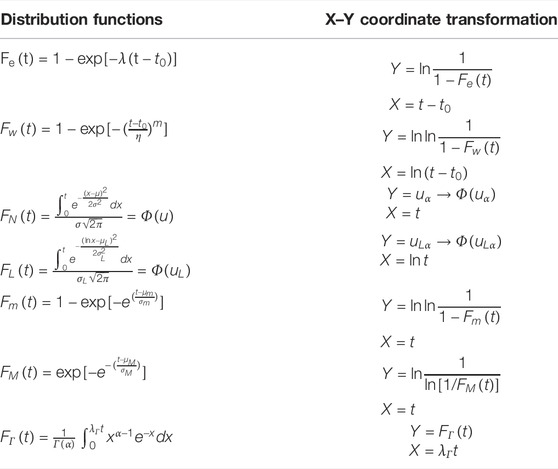
TABLE 2. Design of different probability plots.

To improve the accuracy of statistical inference, the value of $r$ is relatively larger. To reduce the amount of calculation, the life simulation values for the system $t_{Sj},\left(j=\mathrm{1,2},\mathrm{...},r\right)$ are arranged in ascending order of time.

$t_{s\left(1\right)}\le t_{s\left(2\right)}\le \dots \le t_{s\left(j\right)}\le \dots \le t_{s\left(r\right)}.$

Then $\left[t_{s\left(1\right)},t_{s\left(r\right)}\right]$ is evenly divided into p intervals, and p can be determined according to the number of simulations, r, generally $p=20\sim 100$. The time interval is calculated as follows:

$\mathrm{\Delta }{t}_{S,k}=t_{S,k+1}-t_{S,k}k=\mathrm{1,2}\cdots ,p,(7)$

where $t_{S,k+1}$, $t_{S,k}$ is the boundary of the kth interval and $\mathrm{\Delta }{t}_{S,k}$ is the kth interval space.

The median ${\overline{t}}_{S,k}$ of all intervals is denoted as follows:

${\overline{t}}_{S,k}=t_{S,k}+\frac{\mathrm{\Delta }{t}_{S,k}}{2}.(8)$

The frequency number of the life simulation value for the system in the kth interval $\left[t_{S,k+1},t_{S,k}\right]$ is denoted as $r_k$. ${\overline{t}}_{S,k}$, and the corresponding cumulative failure probability constitutes p scattered data pairs $\left[F\left({\overline{t}}_{S,k}\right),{\overline{t}}_{S,k}\right]$.

$\left[F\left({\overline{t}}_{S,k}\right)=\frac{1}{r}\left({\displaystyle \sum _{i=1}^k{r}_i}-\frac{r_k}{2}\right),{\overline{t}}_{S,k}=t_{S,k}+\frac{\mathrm{\Delta }{t}_{S,k}}{2}\right].(9)$

Each scattered data pair $\left[F\left({\overline{t}}_{S,k}\right),{\overline{t}}_{S,k}\right]$ corresponds to 1 point on the probability graph, and the least square method is used to fit the straight line.

$Y_j=a_j+b_j{X}_{j}j=\mathrm{1,2},\cdots ,q,$

where a_j and b_j are the linear parameters of the fitting line, and q is the number of the selected probability graphs.a_j and b_j and the residual sum of squares $Q_j$ are calculated on the probability graph, respectively.

$\{\begin{array}{l}{b}_j=\frac{p{\displaystyle \sum _{k=1}^p{X}_{jk}{Y}_{jk}-}{\displaystyle \sum _{k=1}^p{X}_{jk}{\displaystyle \sum _{k=1}^p{Y}_{jk}}}}{p{\displaystyle \sum _{k=1}^p{X}_{jk}^2-{\left({\displaystyle \sum _{k=1}^p{X}_{jk}}\right)}^2}}\\ a_j=\frac{1}{p}\left[{\displaystyle \sum _{k=1}^p{Y}_{jk}}-b_j{\displaystyle \sum _{k=1}^p{X}_{jk}}\right]\end{array},(10)$

$Q_j={\displaystyle \sum _{k=1}^p{\left(Y_{jk}-a_j-b_j{X}_{jk}\right)}^2},(11)$

where $X_{jk}$ and $Y_{jk}$ are the horizontal and vertical coordinate of the kth data point.

The values of $Q_j$ on different distribution probability graphs are compared, and the distribution corresponding to the minimum value of $Q_j$ is selected as the initial life distribution for the CEMS.

Pearson ${\chi }^2$ Goodness-of-Fit Test

The goodness-of-fit test should be performed after the initial distribution is determined.

The initial distribution function as $F_x\left(t\right)$ is set, and the sample observation is the median value of p intervals, ${\overline{t}}_{S,1},{\overline{t}}_{S,2},\mathrm{...},{\overline{t}}_{S,p}$. The Pearson ${\chi }^2$ goodness-of-fit test is performed as follows:

1) The hypotheses are established.

The original hypothesis $H_0$: the sample is from $F_x\left(t\right)$, and the alternative hypothesis: the sample is not from $F_x\left(t\right)$.

2) The point estimate value $\widehat{{\theta }_x}$ (or ${\widehat{\theta }}_{x1},{\widehat{\theta }}_{x2},\dots ,{\widehat{\theta }}_{xl}$) of $F_x\left(t\right)$ is estimated using the probability graph method.

The probability for p intervals is calculated as follows:

$P_k=F_x\left({\overline{t}}_{S,k+1},{\widehat{\theta }}_x\right)-F_x\left({\overline{t}}_{S,k},{\widehat{\theta }}_x\right)k=\mathrm{1,2}\cdots ,p.(12)$

3) The Pearson ${\chi }^2$ test statistics is calculated by

${\chi }^2={\displaystyle \sum _{k=1}^p\frac{{\left(r_k-r{p}_k\right)}^2}{r{p}_k}}.(13)$

4) When the confidence probability $\gamma$ is given, the following formula holds:

$P\left[{\chi }^2\le {\chi }_{\gamma }^2\left(v\right)\right]=\gamma ,(14)$

where v is the degree of freedom, $v=p-1-l$, and l is the number of parameters of initial distribution.

If ${\chi }^2\le {\chi }_{\gamma }^2\left(v\right)$, the original hypothesis is accepted at a high probability, and then, the sample can be identified from $F_x\left(t\right)$. Otherwise, the original hypothesis shall be rejected.

To facilitate the computer analysis, the Fisher approximation of ${\chi }_{\gamma }^2\left(v\right)$ is given

${\chi }_{\gamma }^2\left(v\right)\approx \frac{1}{2}{\left[\sqrt{2v-1}+u_{\gamma }\right]}^2,(15)$

where $u_{\gamma }$ is the $\gamma$ quantile of the standard normal distribution, which can be approximated as follows:

$u_{\gamma }\approx \frac{a_0+a_{1}z}{1+b_1+b_2{z}^2},(16)$

where a₀ = 2.3075; a₁ = 0.2706; b₁ = 0.9922; b₂ = 0.0448; and $z=\sqrt{\ln {\left(1-\gamma \right)}^{-2}}$.

Engineering Application–System Reliability Prediction on Wind Turbine

An MW wind turbine unit is mainly composed of impeller, gearbox, generator, yaw system, pitch system, brake system, lubrication system, electrical system, and frequency converter in serial connection, and its reliability block diagram (RBD) is shown in Figure 2.

FIGURE 2

FIGURE 2. Reliability block diagram of the wind turbine.

The given life distributions and parameters for all components in the wind power generator unit are listed in Table 3 (Tavner et al., 2007; Spinato et al., 2009; Guo et al., 2012).

TABLE 3

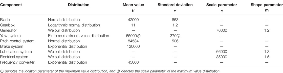
TABLE 3. Distribution parameters of the units.

According to the relevant parameters of each unit listed in Table 3, the life simulation value for each unit is generated using the simulation conversion equation in Table 1. We set $r=500$, and the 500 life simulation values for units are obtained as listed in Table 4 (excerpt). 500 life simulation values for the system are obtained through logical operation.

1) Initial selection of the life distribution types for the wind turbine.

TABLE 4

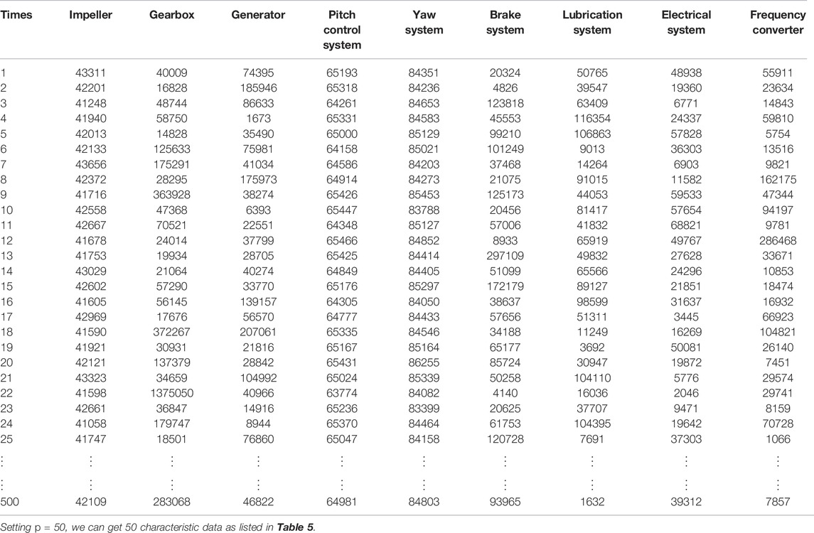
TABLE 4. Units’ life simulation data ($h$).

The characteristic data in Table 5 are processed using probability graph estimation to get the residual sum of squares under different distributions, $Q_j$, as listed in Table 6.

TABLE 5

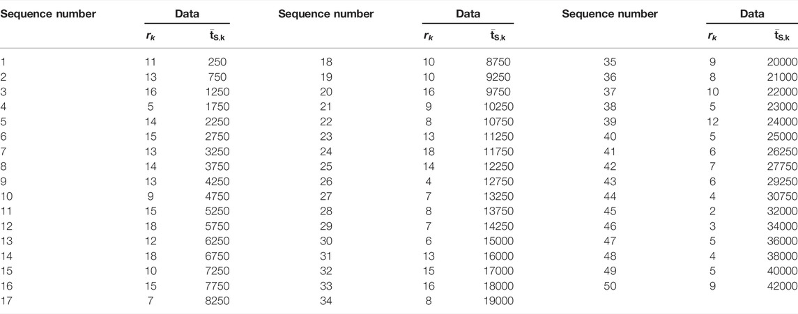
TABLE 5. The system simulation life data.

TABLE 6

TABLE 6. The life distribution deduction result.

It is shown in Table 6 that the residual sum of squares for the two-parameter Weibull distribution was the least, and it can be used as the initial distribution.

2) Goodness-of-fit test for the initial distribution.

According to the probability graph estimation, $m=1.1925$, $\eta =13207h$, the Pearson ${\chi }^2$ test statistics is obtained from Eqs 12 and 13:

${\chi }^2=\mathrm{58.7058.}$

Given the confidence probability $\gamma =0.9$, ${\chi }_{0.9}^2\left(47\right)$ is obtained from Eq. 15.

${\chi }_{0.9}^2\left(47\right)=\mathrm{60.0312.}$

We can obtain ${\chi }^2$ less than ${\chi }_{0.9}^2\left(47\right)$.

${\chi }^2<{\chi }_{0.9}^2\left(47\right).$

The hypothesis test is passed at a high probability, and then the life data of this wind turbine follows the two-parameter Weibull distribution, the distribution parameters, the point estimation and the interval estimation of reliability measures can be further solved.

We set ${\overline{t}}_{S,1},{\overline{t}}_{S,2},\mathrm{...},{\overline{t}}_{S,p}$ as a complete sample, the likelihood function for the two-factor Weibull distribution can be expressed as

$L\left(m,\eta \right)={\displaystyle \prod _{k=1}^p\frac{m}{\eta }}{\left(\frac{{\overline{t}}_{S,k}}{\eta }\right)}^{m-1}\exp \left[-{\left(\frac{{\overline{t}}_{S,k}}{\eta }\right)}^m\right].(17)$

The logarithm is taken from

$\ln L\left(m,\eta \right)=p\ln \frac{m}{\eta }+\left(m-1\right){\displaystyle \sum _{k=1}^p\ln }\frac{{\overline{t}}_{S,k}}{\eta }-{{\displaystyle \sum _{k=1}^p\left(\frac{{\overline{t}}_{S,k}}{\eta }\right)}}^m.(18)$

The constraint conditions are set as

$\frac{\partial \ln L}{\partial m}=0,\frac{\partial \ln L}{\partial \eta }=0.$

The likelihood equations are established and arranged as

$\{\begin{array}{l}\frac{{\displaystyle \sum _{k=1}^p{\left({\overline{t}}_{S,k}\right)}^m\ln {\overline{t}}_{S,k}}}{{\displaystyle \sum _{k=1}^p{\left({\overline{t}}_{S,k}\right)}^m}}-\frac{1}{m}=\frac{1}{p}{\displaystyle \sum _{k=1}^p\ln {\overline{t}}_{S,k}}\\ {\eta }^m=\frac{1}{p}{\displaystyle \sum _{k=1}^p{\left({\overline{t}}_{S,k}\right)}^m}\end{array},(19)$

${\overline{t}}_{S,1},{\overline{t}}_{S,2},\cdots ,{\overline{t}}_{S,50}$ are substituted into Eq. 19 to solve the maximum likelihood estimation for the parameter m, $\eta$.

$\{\begin{array}{l}\widehat{m}=1.2427\\ \widehat{\eta }=13114\end{array}.$

Therefore,

${\overline{T}}_S=\widehat{\eta }\mathrm{\Gamma }\left(1+\frac{1}{\widehat{m}}\right),(20)$

where ${\overline{T}}_S$ is the maximum likelihood estimation for the average life of the wind turbine.

As $\widehat{m}>1$, gamma function can be approximated as

$\begin{array}{l}\mathrm{\Gamma }\left(1+\frac{1}{\widehat{m}}\right)\approx 1-0.5748646\frac{1}{\widehat{m}}+0.9512363{\left(\frac{1}{\widehat{m}}\right)}^2-0.6998588{\left(\frac{1}{\widehat{m}}\right)}^3-\\ 0.6998588{\left(\frac{1}{\widehat{m}}\right)}^3+0.4245549{\left(\frac{1}{\widehat{m}}\right)}^4-0.1010678{\left(\frac{1}{\widehat{m}}\right)}^5.\end{array}(21)$

If $\widehat{m}\le 1$, the calculation can be simplified using the recursive equation and ${\overline{T}}_S$ can be calculated as follows:

${\overline{T}}_S=12287.02h.$

With the given t value, the maximum likelihood estimation for the reliability function $R\left(t\right)$ is

${\widehat{R}}_S\left(t\right)=\exp \left[-{\left(\frac{t}{\widehat{\eta }}\right)}^{\widehat{m}}\right].(22)$

Therefore, the maximum likelihood estimation for the failure rate function $\lambda \left(t\right)$ is

${\widehat{\lambda }}_S\left(t\right)=\frac{\widehat{m}}{\widehat{\eta }}{\left(\frac{t}{\widehat{\eta }}\right)}^{\widehat{m}-1}.(23)$

If the confidence probability is set as $1-\alpha$, the confidence interval for the distribution parameter m, $\eta$ is

$\{\begin{array}{l}{m}_L=\widehat{m}\exp \left(-u_{1-\frac{\alpha }{2}}\frac{1.0490}{\sqrt{p-1}}\right)\\ m_U=\widehat{m}\exp \left(u_{1-\frac{\alpha }{2}}\frac{1.0490}{\sqrt{p-1}}\right)\end{array},(24)$

$\{\begin{array}{l}{\eta }_L=\widehat{\eta }\exp \left(-u_{1-\frac{\alpha }{2}}\frac{1.0810}{\widehat{m}\sqrt{p-1}}\right)\\ {\eta }_U=\widehat{\eta }\exp \left(u_{1-\frac{\alpha }{2}}\frac{1.0810}{\widehat{m}\sqrt{p-1}}\right)\end{array},(25)$

where $u_{1-\frac{\alpha }{2}}$ is the quantile of standard normal distribution, and it can be calculated by Eq. 16.

To simplify the calculation, the shape parameter m can be taken as its maximum likelihood estimation, and it is taken as $\widehat{m}=1.2427$.

When the given confidence probabilities $1-\alpha$ are 0.9, 0.8, and 0.7, respectively, the confidence interval for the distribution parameter m, $\eta$, and lower confidence limit for the average life of the wind turbine are shown in Table 7.

${\left(R_S\left(t\right)\right)}_L=\exp \left[-{\left(\frac{t}{{\eta }_L}\right)}^{\widehat{m}}\right].(26)$

TABLE 7

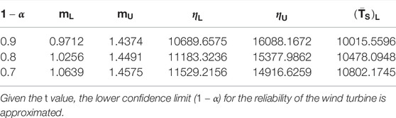
TABLE 7. The confidence interval for the distribution parameter and lower confidence limit for the average life of the wind turbine under different confidence probabilities.

The upper confidence limit ($1-\alpha$) for its failure rate is approximated as

${\left({\lambda }_S\left(t\right)\right)}_U=\frac{\widehat{m}}{{\eta }_L}{\left(\frac{t}{{\eta }_L}\right)}^{\widehat{m}-1}/\mathrm{h},(27)$

when t is 1000, 1500, 2000, 2500, and 3000h, and the confidence probabilities $1-\alpha$ are 0.9, 0.8, and 0.7, respectively, the reliability lower confidence limit ($1-\alpha$) and failure rate upper confidence limit ($1-\alpha$) of wind turbine are shown in Figure 3 and Figure 4, respectively.

FIGURE 3

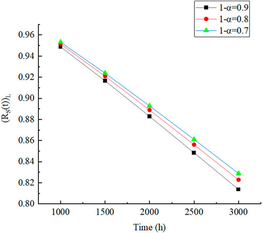
FIGURE 3. Reliability lower confidence limit ($1-\alpha$) of the wind turbine under different confidence probabilities and life.

FIGURE 4

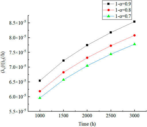
FIGURE 4. Failure rate upper confidence limit ($1-\alpha$) of the wind turbine under different confidence probabilities and life.

It can be seen from Figure 3 and Figure 4 that all lower limits of reliability ${\left(R_S\left(t\right)\right)}_L$ show a downward trend, while all failure rates show an upward trend under different confidence probabilities.

Conclusion

For the CEMS with many limiting factors, this article presented a method of replacing life test with computer analog simulation for CEMS. The life simulation values of system constituent units of CEMS could be obtained by their life distribution types and relevant distribution parameters. The life simulation values of CEMS were obtained according to the reliability logic relationship and reliability logic block diagram of the CEMS, and the simulation was instead of the life test of CEMS when the simulation times were enough. The method proposed in this thesis was of great significance to save test time and test cost, especially for the CEMSs that could not carry out reliability life test.

The method proposed in this thesis could solve the problems of system reliability synthesis and prediction of CEMS with different distributions of units. When the “pyramid model” was used for system reliability level by level synthesis and prediction. Compared with the traditional life test method of CMES, it could save a lot of test cost, test time, test site, and so on. This approach could be applied to the early program design, prototype development, trial production, and other stages of production. In engineering applications, the CMES reliability logic block diagram could be drawn by computer, and all the smallest path sets could be obtained by the node traversal optimization algorithm. Therefore, it has obvious application value in engineering.

Finally, the proposed method was applied to the wind turbine, and the reliability lower confidence limit ($1-\alpha$) and failure rate upper confidence limit ($1-\alpha$) of wind turbine were calculated with given the life time t. The method is also applicable to other CEMSs and can be utilized to provide guidance for system design, maintenance planning, and so on. This paper provides an effective and flexible method for reliability synthesis and prediction of CEMS, which can be easily implemented in engineering practices.

Data Availability Statement

The raw data supporting the conclusions of this article will be made available by the authors, without undue reservation.

Author Contributions

CY: writing, reviewing, and editing, YG: reviewing and drawing, and XY: funding acquisition.

Funding

This work was supported by the project of the Natural Science Foundation of Shandong Province, China (No. ZR2019PEE018) and Shandong Province Science and Technology SMES Innovation Ability Enhancement Project (No. 2021TSGC1063).

Conflict of Interest

The authors declare that the research was conducted in the absence of any commercial or financial relationships that could be construed as a potential conflict of interest.

Publisher’s Note

All claims expressed in this article are solely those of the authors and do not necessarily represent those of their affiliated organizations, or those of the publisher, the editors, and the reviewers. Any product that may be evaluated in this article, or claim that may be made by its manufacturer, is not guaranteed or endorsed by the publisher.

Acknowledgments

The authors thank all the editors and referees for their helpful suggestions.

References

Aguwa, J. I., and Sadiku, S. (2012). Reliability Studies on Timber Data from Nigerian Grown Iroko Tree (Chlorophora Excelsa) as Bridge Beam Material. Jera 8 (12), 17–35. doi:10.4028/www.scientific.net/jera.8.17

CrossRef Full Text | Google Scholar

Buehler, R. J. (1957). Confidence Intervals for the Product of Two Binomial Parameters. J. Am. Stat. Assoc. 52 (280), 482–493. doi:10.1080/01621459.1957.10501404

CrossRef Full Text | Google Scholar

Cancela, B., Ortega, M., Penedo, M. G., Novo, J., and Barreira, N. (2013). On the Use of a Minimal Path Approach for Target Trajectory Analysis. Pattern Recognition 46 (7), 2015–2027. doi:10.1016/j.patcog.2013.01.013

CrossRef Full Text | Google Scholar

Fo, X. C., and Xiong, H. L. (2009). MML Method and its Application in the Reliability Analysis of Navigating System. Electron. Product. Reliability Environ. Test. 27 (1), 16–19. doi:10.3969/j.issn.1672-5468.2009.01.005

CrossRef Full Text | Google Scholar

Fuqiu, L., Wang, Z., Xiaopeng, L., and Zhang, W. (2020). A Reliability Synthesis Method for Complicated Phased Mission Systems[J]. IEEE Access 8, 193681–193685. doi:10.1109/ACCESS.2020.3028303

CrossRef Full Text | Google Scholar

Graves, T. L., and Hamada, M. S. (2016). A Note on Incorporating Simultaneous Multi-Level Failure Time Data in System Reliability Assessments. Qual. Reliab. Engng. Int. 32, 1127–1135. doi:10.1002/qre.1820

CrossRef Full Text | Google Scholar

Guo, J., Sun, Y., and Wang, M. (2012). System Reliability Synthesis of Wind Turbine Based on Computer Simulation[J]. J. Mech. Eng. 48 (2), 1–7. doi:10.3901/JME.2021.02.002

CrossRef Full Text | Google Scholar

Guo, J., Sun, Y., Yu, C., Yuan, H., and Su, Z. (2014). Some Theory and Method for Complex Electromechanical System Reliability Prediction[J]. J. Mech. Eng. 50 (4), 1–13. doi:10.3901/jme.2014.14.001

CrossRef Full Text | Google Scholar

Guo, J., and Wilson, A. G. (2013). Bayesian Methods for Estimating System Reliability Using Heterogeneous Multilevel Information. Technometrics 55 (4), 461–472. doi:10.1080/00401706.2013.804441

CrossRef Full Text | Google Scholar

Han, S.-Y., Zhou, J., Chen, Y.-H., Zhang, Y.-F., Tang, G.-Y., and Wang, L. (2021). Active Fault-Tolerant Control for Discrete Vehicle Active Suspension via Reduced-Order Observer. IEEE Trans. Syst. Man. Cybern, Syst. 51 (11), 6701–6711. doi:10.1109/tsmc.2020.2964607

CrossRef Full Text | Google Scholar

Hong-Bo, Z., and Guo, J. (2009). Method of System Reliability Synthesis Based on Minimal Path Sets[J]. Transducer Microsystem Tech. 28 (8), 20–23. doi:10.13873/j.100-97872009.08.14

CrossRef Full Text | Google Scholar

Kovacs, Z., Orosz, A., and Friedler, F. (2019). Synthesis Algorithms for the Reliability Analysis of Processing Systems. Cent. Eur. J. Oper. Res. 27, 573–595. doi:10.1007/s10100-018-0577-0

CrossRef Full Text | Google Scholar

Liu, Y., Zuo, M. J., Li, Y.-F., and Huang, H.-Z. (2015). Dynamic Reliability Assessment for Multi-State Systems Utilizing System-Level Inspection Data. IEEE Trans. Rel. 64 (4), 1287–1299. doi:10.1109/tr.2015.2418294

CrossRef Full Text | Google Scholar

Meng, J., and Wen-Tao, Z. (2021). Research on the Reliability of Differential Protection Based on Monte Carlo[J]. Computer Simulation 38 (11), 112–116. doi:10.3969/j.issn.1006-9348.2021.11.023

CrossRef Full Text | Google Scholar

Mi, J., Li, Y. F., Yang, Y. J., Peng, W., and Huang, H. Z. (2016). Reliability Assessment of Complex Electromechanical Systems under Epistemic Uncertainty. Reliability Eng. Syst. Saf. 152 (8), 1–15. doi:10.1016/j.ress.2016.02.003

CrossRef Full Text | Google Scholar

Negi, S., and Singh, S. B. (2015). Reliability Analysis of Non-repairable Complex System with Weighted Subsystems Connected in Series. Appl. Math. Comput. 262 (262), 79–89. doi:10.1016/j.amc.2015.03.119

CrossRef Full Text | Google Scholar

Peng, W., Huang, H., Xie, M., Yang, Y., and Liu, Y. (2013). A Bayesian Approach for System Reliability Analysis with Multilevel Pass-Fail, Lifetime and Degradation Data Sets. IEEE Trans. Rel. 62 (3), 689–699. doi:10.1109/tr.2013.2270424

CrossRef Full Text | Google Scholar

Praks, P., and Gono, R. (2011). “Uncertainty Analysis of Failure Rate of Selected Transformers in a Power Distribution Network[C],” in Proceedings of the 12th International Scientific Conference Electric Power Engineering 2011, EPE 2011, 645–648.

Google Scholar

Schallert, C. (2014). A Safety Analysis via Minimal Path Sets Detection for Object-Oriented Models. ESREL, 2019–2027. doi:10.1201/b17399-277

CrossRef Full Text | Google Scholar

Spinato, F., Tavner, P. J., Bussel Van, G. J. W., and Koutoulakos, E. (2009). Reliability of Wind Turbines Subassemblies [J]. IET Renew. Power Generator 3 (4), 1–15. doi:10.1049/iet-rpg.2008.0060

CrossRef Full Text | Google Scholar

Sun, Y., Sun, T., Pecht, M. G., and Yu, C. (2018). Computing Lifetime Distributions and Reliability for Systems with Outsourced Components: A Case Study. IEEE Access 6, 31359–31366. doi:10.1109/access.2018.2843375

CrossRef Full Text | Google Scholar

Tang, S., Zhu, Y., and Yuan, S. (2021). An Improved Convolutional Neural Network with an Adaptable Learning Rate towards Multi-Signal Fault Diagnosis of Hydraulic Piston Pump. Adv. Eng. Inform. 50, 101406. doi:10.1016/j.aei.2021.101406

CrossRef Full Text | Google Scholar

Tavner, P. J., Xiang, J., and Spinato, F. (2007). Reliability Analysis for Wind Turbines. Wind Energy 10, 1–18. doi:10.1002/we.204

CrossRef Full Text | Google Scholar

Wang, H., Gong, Z., Huang, H. Z., Xiaoling, Z., and Zhiqiang, Lv. (2012). “System Reliability Based Design Optimization with Monte Carlo Simulation[C],” in 2012 International Conference on Quality, Reliability, Risk, Maintenance, and Safety Engineering, Chengdu, China, 15-18 June 2012, 1143–1147.

Google Scholar

Wang, Y., Zhou, J., Wang, R., Chen, L., Zhang, T., Han, S., et al. (2022). Transfer Collaborative Fuzzy Clustering in Distributed Peer-To-Peer Networks[J]. IEEE Trans. Fuzzy Syst. 30 (2), 500–514. doi:10.1109/TFUZZ.2020.3041191

CrossRef Full Text | Google Scholar

Weiyan, M., Xingzhong, X., and Shifeng, X. (2009). Inference on System Reliability for Independent Series Components[J]. Commun. Statistics-Theory Methods 38 (3), 409–418. doi:10.1080/03610920802220793

CrossRef Full Text | Google Scholar

Wilson, A. G., Graves, T. L., Hamada, M. S., and Reese, C. S. (2006). Advances in Data Combination, Analysis and Collection for System Reliability Assessment[J]. Stat. Sci. 21 (4), 514–531. doi:10.1214/088342306000000439

CrossRef Full Text | Google Scholar

Yeh, W., Lin, Y., Chung, Y., and Mingchang, C. (2010). A Particle Swarm Optimization Approach Based on Monte Carlo Simulation for Solving the Complex Network Reliability Problem. IEEE Trans. Rel. 59 (1), 212–221. doi:10.1109/tr.2009.2035796

CrossRef Full Text | Google Scholar

Yoshida, I., and Akiyama, M. (2011). “Reliability Estimation of Deteriorated RC-Structures Considering Various Observation Data[C],” in 11th International Conference on Applications of Statistics and Probability in Civil Engineering, 1231–1239. doi:10.1201/b11332-187

CrossRef Full Text | Google Scholar

Yu, C., Guo, J., Sun, Y., Su, Z., and Yuan, H. (2013). Bayes Confidence Limit of Reliability for Series-Parallel System Consisting of Different Distribution Units[J]. Chin. J. Scientific Instrument 34 (2), 428–433. doi:10.19650/j.cnki.cjsi.2013.02.028

CrossRef Full Text | Google Scholar

Yuan, R., Tang, M., Wang, H., and Li, H. (2019). A Reliability Analysis Method of Accelerated Performance Degradation Based on Bayesian Strategy. IEEE Access 7, 169047–169054. doi:10.1109/ACCESS.2019.2952337

CrossRef Full Text | Google Scholar

Zhang, M., Hu, Q., Xie, M., and Yu, D. (2014). Lower Confidence Limit for Reliability Based on Grouped Data Using a Quantile-Filling Algorithm. Comput. Stat. Data Anal. 75 (75), 96–111. doi:10.1016/j.csda.2014.01.010

CrossRef Full Text | Google Scholar

Zhou, Y. Q., and Weng, Z. X. (1990). Reliability evaluation[M]. Beijing: Science Press.

Google Scholar

Zhu, X. B., and J Sh, L. (1990). Combined MML & SR Method (CMSR) for System Reliability Assessment. J. Astronautics (2), 29–34.

Google Scholar