Best Practices in PEC Water Splitting: How to Reliably Measure Solar-to-Hydrogen Efficiency of Photoelectrodes

Introduction

Purpose of This Protocol

This protocol aims to provide guidance on the best practices for benchmarking the solar-to-hydrogen (STH) efficiency of photoelectrochemical (PEC) materials. STH efficiency is a key metric for judging the quality of new PEC materials and their feasibility for implementation in practical water-splitting devices. Direct measurement of hydrogen generated by the PEC material is required for an accurate characterization of STH efficiency. Some materials developed for water splitting may have low photocurrents, require an applied voltage to produce hydrogen, or have a lifetime too short to measure generated hydrogen. They still can be characterized by other metrics such as photocurrent density and device lifetime, but in that case STH efficiency values cannot be extrapolated from the measured current density, nor compared with others. In addition to communicating the need for this direct measurement, it is hoped that improved uniformity of experimental practices for performing this key measurement will facilitate the development of new materials.

The STH efficiency (η_STH) is calculated as follows:

${\text{η}}_{\text{STH}}=\frac{{\text{j}}_{\text{sc}}\left(\frac{\text{mA}}{{\text{cm}}^2}\right)\text{∗}1.23{\text{ V∗ η}}_{\text{F}}}{{\text{P}}_{\text{total}}\left(\frac{\text{mW}}{{\text{cm}}^2}\right)}.(1)$

Therefore, accurate calculation of η_STH relies on an accurate measurement of j_sc (photocurrent density at short circuit) and η_F (the system Faradaic efficiency), and calibration of P_total (the power density of the light source illuminating the sample). In Eq. 1, 1.23 V is the potential difference necessary to generate H₂ and O₂ under standard conditions (25°C). η_F can be defined as the quantity of hydrogen produced for a given current supplied

${\text{η}}_{\text{F},\text{ H}2}=\frac{\left({\text{H}}_2\text{produced}\right)}{\left(\text{measured current}\right)}=\frac{\left(\frac{\text{mol}}{\text{s}}{\text{H}}_2\text{∗}\frac{2{\text{e}}^{-}}{{\text{H}}_2}\text{∗F}\left(\frac{\text{C}}{\text{mol}}\right)\right)}{\text{I }\left(\text{A}\right)}.(2)$

The accurate measurement of P_total, H₂ produced, measured current, and measured current density requires attention to equipment calibration and sample preparation. These topics will be discussed in the remainder of this protocol. In addition, we will present the best practices for measuring and reporting the broadband and monochromatic photocurrent response of a material, considering spatial variability and reproducibility of the material fabrication, and the effect of the measurements on the material. Finally, durability measurements, combined with η_STH calculations to determine device lifetime, will be briefly discussed. Previously published guidelines for efficiency determination and reporting for PEC devices are presented in Chen et al. (2011) and in more detail in Chen et al. (2013).

PEC Experimental Design and Data Reporting

Prior to η_STH measurements, initial material characterization should be done by measuring the photocurrent of a representative sample of the synthesized PEC material under broadband and monochromatic light, to determine the reproducibility and variability of photocurrent. The order of broadband and monochromatic measurements on the photoelectrode pieces should be randomized to detect if one measurement affects the other. For example, if a representative sample of 10 is selected for each material, the monochromatic response is measured first in 5 of the 10, and the broadband response is measured first in the other 5. If a systematic discrepancy is seen between the two datasets, troubleshooting is warranted to decrease corrosion caused by the measurement. If no discrepancy is seen, the statistical robustness of the results will be strengthened.

As another consideration for experimental design, the variability of performance of a new PEC material—within each batch and between synthetic batches—should be reported. Many complex solar absorbers representing the top tier of the current PEC performance show varied performance between synthetic batches, so it remains important for the field to report not only the best result but also the average and range of measured efficiencies for a series of nominally identical syntheses. Many synthetic methods also display variability within the area of one growth/deposition. For example, there is often variation in layer thickness/quality between the center and the edge of the substrate for growth methods such as metalorganic vapor-phase epitaxy (MOVPE) and electrodeposition, as well as deposition from solution by spin coating. Physical vapor deposition and sputtering can also result in non-uniformities across the width of the substrate. Therefore, the sample selected from each batch should be selected to be truly representative of the spatial variability present for a given fabrication method.

Outliers should be removed from the dataset only in extreme cases. For instance, if the edge pieces for a wafer grown by MOVPE are systematically worse than the center pieces, they can be habitually discarded and not tested. While, in this protocol, we have looked at a specific synthetic methodology (MOVPE), considerations with respect to the utilized synthetic routes should be considered when defining outliers. For example, heterogeneities on samples can originate during sputtering deposition and electrodeposition or by deposition of pre-synthesized powders. In all these cases, our recommendation is to perform a combination of characterizations of photophysical, chemical, and photoelectrochemical properties on different sample regions. In addition, some surface modifications treat an entire undivided wafer (e.g., sputtering) while others, such as electrodeposition, are typically done on individual electrodes. In both cases, multiple electrodes from nominally identical treatments should be measured, compared, and reported. This approach should help in the outliers’ determination and may provide feedback on improving the deposition/fabrication of the photoelectrodes.

It is also important to mention that choosing the appropriate electrolyte, with respect to pH, requires consideration of the kinetic influence on performance and the chemistry of decomposition reactions on durability. In order to achieve maximum efficiency, a photocathode should be operated in an acidic electrolyte where the hydrogen evolution reaction (HER) is favored. Conversely, a photoanode should be operated in basic solution, where the oxygen evolution reaction (OER) is most kinetically favored. The choice of electrolyte pH for best overall performance is more nuanced. Some research groups have achieved higher durability in neutral, buffered electrolytes. However, these results come at the expense of a diminished efficiency due to kinetic factors, increased solution resistance, and the buildup of a pH gradient with time (Xu et al., 2021). Therefore, we recommend using an electrolyte that balances all of the above considerations and reporting the justification for its selection. If different electrolytes are used, for example, acid for photocathode efficiency and neutral for durability measurements, those details should be explicitly reported, as well included as part of the discussion of results.

Overview of the Remainder of the Document

With a focus on the characterization and η_STH benchmarking of a new photocathode material, this protocol is based on established best practices developed at LBNL (Lawrence Berkeley National Laboratory) and NREL (National Renewable Energy Laboratory) (Chen et al., 2011; Steiner et al., 2012; Chen et al., 2013; Döscher et al., 2016; Young et al., 2017). First, the fabrication of photoelectrodes to probe the performance and statistics of a new PEC material is shown, followed by broadband and monochromatic photocurrent testing of each electrode and suggestions to probe material durability. In this context, we also describe the calibration of light sources. Finally, methods for consistently testing η_F and η_STH will be provided, along with examples of their measurement. The testing vessel used herein for measuring η_F and η_STH is a sealed compression cell that accommodates a 1 cm² photoelectrode, and its assembly will also be described. Finally, there will be a brief discussion of durability testing, which allows tracking η_STH over time.

III–V Tandem Photoabsorber Example

To describe the steps of this protocol, we will use, as a model example, a III–V tandem photocathode material with GaInP and GaAs junctions that have band gaps of ∼1.8 eV (GaInP) and ∼1.4 eV (GaAs). In a cell with sufficient ionic conductivity and appropriate hydrogen and oxygen evolution catalysts, this material can evolve hydrogen under 1-sun illumination without externally applied bias. The structure of the photocathode is shown in Figure 1, with similar tandem photocathode materials having been previously reported (Döscher et al., 2016; Young et al., 2017). Note that the metallic back contact was deposited after growth.

FIGURE 1

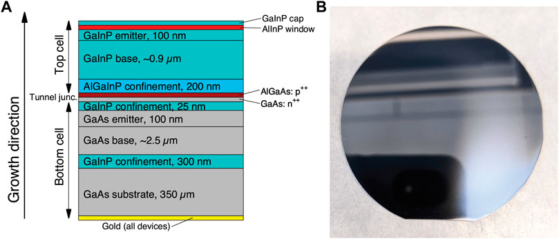
FIGURE 1. Tandem photoabsorber architecture. (A) The vertical structure of layers in the III–V tandem photocathode characterized in this document. (B) A 2″ wafer of (A), GaInP top surface.

PEC Electrode Fabrication and Integrated Testing Vessel

This section discusses the fabrication details of photoelectrodes for material characterization and assembly of the integrated testing vessel for η_F measurements. We provide detailed information about the material we tested to show a prototypical example for a procedure that can be adaptable and amenable to many different material systems.

Radial Strip Photoelectrodes: Fabrication and Area Determination

For PEC materials grown on wafers by MOVPE, as the III–V tandem photocathode was, the full diameter of the wafer should be characterized to probe the spatial variation in the material growth quality between the edge and center. Here, we take a 5 mm wide strip from the center of the 2″ wafer, as shown in Figures 2A,B, and divide it into ten 5 × 5 mm squares. After obtaining the 5 × 5 mm squares, the next step in the photoelectrode fabrication is mounting each square on a glass handle for ease of PEC testing. For PEC materials deposited by other methods and on other substrates, a representative sample should be tested by considering the variations introduced by processing methodologies.

FIGURE 2

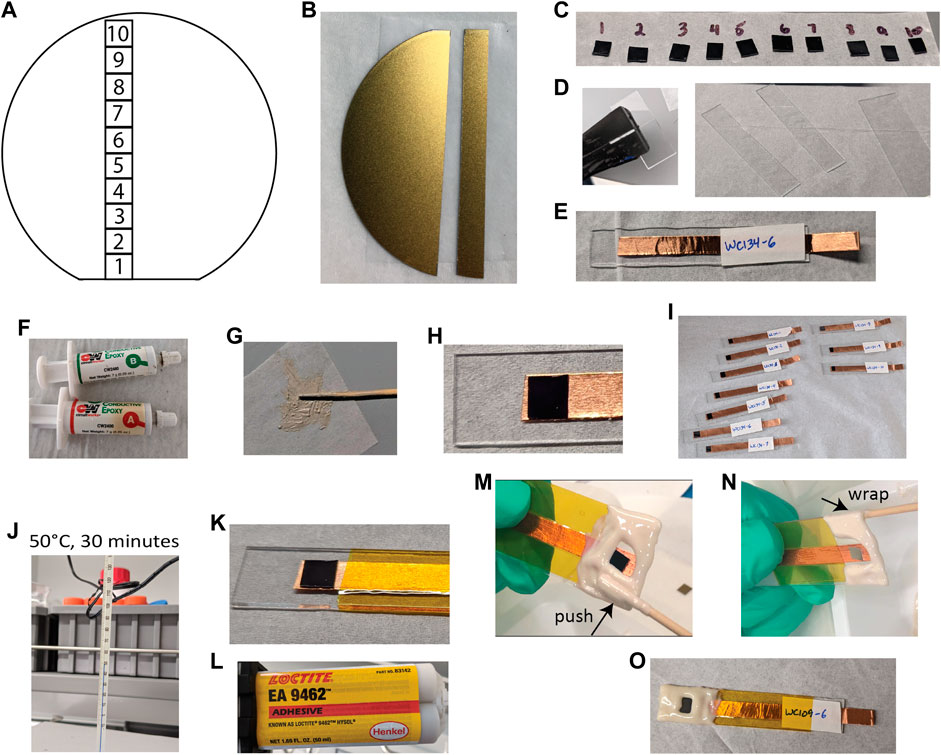
FIGURE 2. Photoelectrode preparation. (A) Schematic of a 2″ wafer showing ten 5 × 5 mm squares in a radial strip. (B) A 5 mm strip cleaved from a GaInP/GaAs wafer, showing back ohmic contact. (C) 5 × 5 mm squares from the wafer. (D) Running pliers and prepared glass slide handles. (E) Copper tape and label applied to one handle. (F) CircuitWorks CW2400 silver epoxy. (G) Prepared silver epoxy. (H) 5 mm square adhered to copper tape with a small amount of silver epoxy. (I) Ten electrodes prepared for curing. (J) Electrodes are cured at 50°C for 30 min. (K) Kapton tape added to cover most of the exposed tape. (L) Loctite EA 9462 epoxy. (M,N) Defining surface area and sealing photoelectrode edges. (O) Completed electrodes after 24 h of curing EA 9462 epoxy.

Experimental Setup

The following components are needed for the fabrication of photoelectrodes:

1. Photoelectrode material or tandem junction with or without suitable catalyst deposited.

2. 1″ × 3″ glass microscope slides.

3. Diamond scribe.

4. Glass running pliers.

5. ¼″ copper tape (or other conductive tape).

6. For materials without an existing ohmic back contact: indium-gallium (InGa) eutectic (e.g., from Thermo Scientific or Millipore Sigma) and InGa-dedicated diamond scribe.

7. Silver epoxy (CircuitWorks CW2400).

8. ½″ or 1″ Kapton tape.

9. Non-conductive epoxy (opaque, e.g., Loctite Hysol EA 9462, or transparent, e.g., Epo-Tek 302-3M) that is compatible with the electrolyte planned.

10. Plastic-tipped tweezers to avoid metal contamination.

11. 50°C oven for curing.

12. Computer hardware and software for area determination including a flatbed scanner (resolution at least 1200 dpi) and a computer with free ImageJ software installed.

Photoelectrode Fabrication Procedure

The workflow for the photoelectrode fabrication is summarized in Figure 2 and described as follows:

1. Cut 5 mm squares of the PEC material. If starting with a crystalline wafer, one option is to place it facedown on a scratch-free surface such as lens paper and then isolate a 5 mm strip by lightly scoring a line down the back with a diamond scribe, guided by a glass slide or cover slip. Then, grip the edge on either side of the line with forceps or gloved fingers, and gently flex away from the score until it breaks. For many wafers, a tick mark at the edge is sufficient rather than a full score—the required method for neatly dicing the material under study should be tested on a small piece first. For glass or FTO/ITO substrate, dice in the same way as for glass slides (see below), being mindful to not cause damage to the deposited material. Figure 2C shows 5 mm squares cut from a radial strip of a GaInP/GaAs wafer.

2. Prepare the glass handles for the electrodes (Figure 2D). The handle width depends on the particular testing vessel planned for the PEC measurements--if there is 1″ or ½″ opening. For a ½″ wide handle, score a glass slide lengthwise once only, with firm pressure, using a diamond scribe and ruler, and break along the score with running pliers. For a 1″ wide handle, use an entire glass slide for each electrode.

3. Cut a piece of copper tape slightly longer than the microscope slide, then remove the paper backing, apply lengthwise to the middle of the glass, and stop around 5–10 mm short of one end. Fold the other end over to provide a connection for an alligator clip (Figure 2E). Repeat to prepare handles for as many electrodes as desired. Label each electrode with a unique identifier.

4. If the back of the material does not have an integrated ohmic contact and forms a native oxide layer (e.g., a Si substrate), apply a small amount of InGa eutectic, then scratch lightly with the InGa-dedicated diamond scribe, and remove the native oxide layer while spreading the eutectic to form an ohmic contact. This can result in a better electrical contact than scratching through the oxide first, followed by InGa application, because SiO₂ and other native oxides begin to reform quickly after exposure to air.

5. To connect the ohmic contact to the copper tape, mix a small amount of two-part silver epoxy, such as CW2400, on a piece of weighing paper using a wooden applicator (Figures 2F,G). Apply a minimal amount to the copper tape near the end, and place the 5 mm square ohmic contact down onto the silver epoxy, leveling by pressing the corners with plastic-tipped tweezers (Figure 2H). Caution: if too much silver epoxy is applied, leading to it contacting the edges of the sample, a short may occur, or the components of the silver epoxy may create additional features in the current density-voltage (J-V) curves. Apply only as much as needed to adhere to the sample. If the epoxy is observed to ooze up the edges of the sample after it is pressed down, too much has been added.

6. Place samples in an oven to cure (50°C for 30 min, when using CW2400) (Figure 2J).

7. After the silver epoxy is cured, remove the electrodes from the oven and apply Kapton tape to tightly cover most of the copper tape (Figure 2K). Covering more of the tape here decreases the amount of epoxy needed in the next step.

8. Use the non-conductive epoxy to seal the remainder of the copper tape and the electrode edges from the electrolyte. Mix Loctite Hysol EA 9462 (Figure 2L) or another inert epoxy in a weigh boat or the other suitable surface with a separate wooden applicator (not the same one used for the silver epoxy to avoid inadvertent contamination with conductive particles), and spread the mixed epoxy to cover the edges of the photoelectrode. Roll the applicator, push a thick ridge of epoxy slightly over the photoelectrode edges to create a good surface area definition (Figure 2M), and wrap the epoxy slightly around the edges of the glass handle to create a good seal (Figure 2N). While defining the surface area, leave as large an exposed surface area as possible while still sealing the edges from electrolyte exposure. A well-defined edge is particularly important if the epoxy around the electrode surface is nominally opaque yet appears transparent when applied in a thin layer. Transparency at the edges will lead to area underestimation of the surface area that is exposed to light and, therefore, overestimation of current density. (For the purposes of this protocol, we neglect the imperfect transparency of “transparent epoxy” at short wavelengths.)

9. Allow Loctite 9462 epoxy to cure at room temperature overnight or allow other epoxy to cure as stated. A better quality of cured epoxy may be obtained for 9462 if done at room temperature rather than elevated temperature.

Illuminated Area Measurement

The electrode area exposed to electrolyte and/or illumination is directly proportional to the magnitude of the photocurrent. Therefore, it is important to accurately and consistently measure the exposed surface area of each electrode prior to commencing PEC measurements.

Once the epoxy is cured, the exposed geometric surface area must be measured, with the process summarized in Figure 3. A flatbed scanner is recommended for this purpose because it is accurate and typically readily available. Other imaging techniques, as long as they provide high resolution and are accurate, can be used to determine the area. One example is a camera with a macro lens, immobilized and calibrated at a set distance from the test surface and with corrections for lens distortion (Dunbar et al., 2015). Note: If instead of a nominally opaque epoxy, a transparent epoxy such as Epo-Tek 302-3M is used to seal the photoelectrode, the entire 5 mm square area will be used to calculate the current density. However, the surface should still be scanned to measure the 5 mm square area accurately.

1. Place the electrode on the flatbed scanner, so the electrode surface is held parallel to the scanner glass, and scan in grayscale with at least 1200 dpi resolution. Save as a .tif file. Lower resolution scans should not be used for measuring the surface area because they can introduce errors by the pixilation of the boundary between the electrode surface and the epoxy surface.

2. From the resolution of the scan, calculate the number of pixels/cm² as (dpi/2.54)². For example, for 2400 dpi, the conversion is 892802 pixels/cm².

3. Install free ImageJ software if not already installed. Load the scanned .tif file into ImageJ, and then select a region around the electrode surface with the rectangle tool and crop the image (Ctrl + Shift + X) (Figure 3A).

4. Find the surface of the electrode bordered by epoxy. Select Image > Adjust > Threshold (Ctrl + Shift + T), and move the bottom slider such that the red region covers the electrode area, leaving the area covered with epoxy gray. Click “Apply” (Figure 3B).

5. Select the electrode area with the magic wand tool and then Edit > Fill, and Edit > Clear Outside (Figure 3C).

6. Count the pixels using the histogram tool: Select Analyze > Histogram (Ctrl + H), observe if the electrode area corresponds to 0 or 255 on the grayscale, and then click “List” to get a count of the number of black and white pixels (Figure 3D). Divide the pixel count of the electrode surface area by the pixels/cm² from the scanner resolution to get the electrode surface area in square centimeters (Figure 3E). Alternatively, select Analyze > Measure to obtain the pixel count.

FIGURE 3

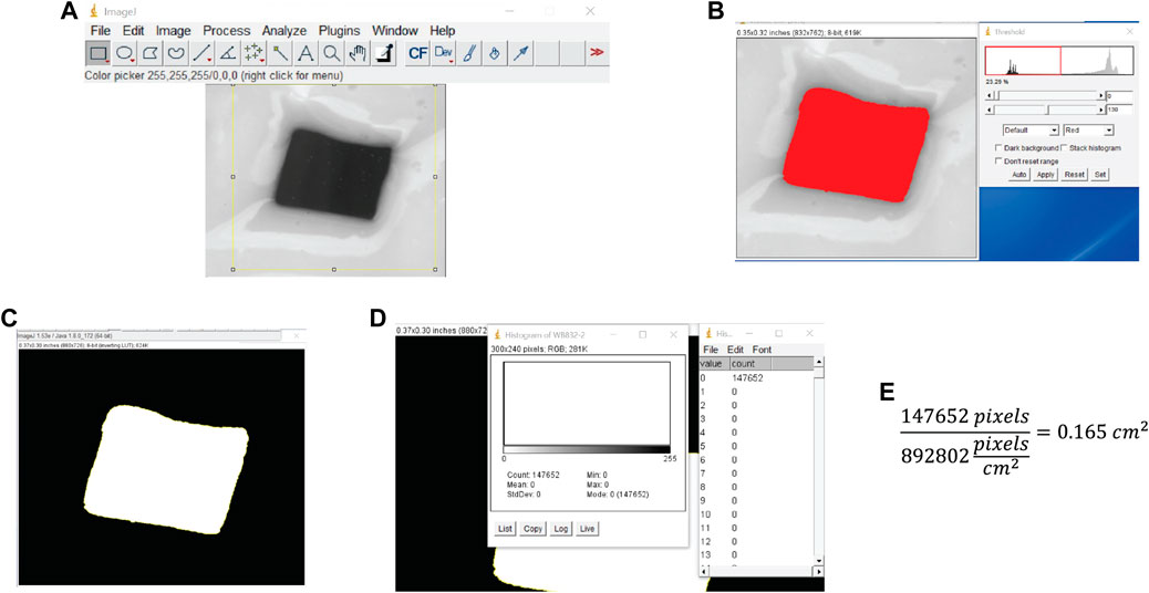
FIGURE 3. Test electrode area determination. (A) Image is cropped to isolate the electrode surface. (B) The threshold is set by adjusting the slider to fill the entire electrode area while excluding surrounding epoxy. (C) The area is selected and filled to get a black and white image. (D) The number of pixels in the electrode surface area is determined using the histogram. (E) The surface area is computed by dividing the number of pixels in the surface area by the scan resolution in pixels/cm².

To quantify the PEC properties of each electrode, skip to the section on PEC measurements. To perform testing vessel assembly for η_STH measurement of a 1 cm² sample, continue with Photoelectrode Integration section.

Photoelectrode Integration Into η_STH Testing Vessel

In order to measure the η_STH for a photocathode, the hydrogen produced must be accurately quantified while simultaneously measuring the photocurrent. To quantify the evolved hydrogen, gas chromatography (GC) should be used. To prevent leakage of H₂ and O₂ after their generation and separation, a well-sealed testing vessel is needed, which incorporates the photocathode (working electrode, or WE), counter electrode (CE), and a membrane separating the anode and cathode chambers. A reference electrode (RE) can be used for measuring η_F of a catalyst but should not be used in measuring or reporting η_F or η_STH of an integrated photocathode. In a PEC device deployed in the field, the anode and cathode compartments will be separated by a proton exchange membrane (PEM) or anion exchange membrane (AEM), depending on the pH of the electrolyte, to allow the collection of H₂ and O₂ without risking their loss or reaction through recombination. Because the membrane will have a potential drop across it, the presence of a membrane will change the output characteristics compared to a PEC cell with no membrane, and higher potentials may be needed for the integrated cell when a membrane is used. Therefore, the membrane separating the compartments is an integral part of accurately measuring η_STH, and the testing vessel used must accommodate it.

In this protocol, we use a testing vessel that accommodates a 1 cm² surface area photocathode and dual anode chambers, with the anodes oriented at 90° angles to the photocathode (Figure 4). Dual anodes and the 90° orientation between the photocathode and each anode are chosen to minimize asymmetric corrosion of the photocathode during a stability test. Compared to the 5 mm squares used in the previous section, the larger surface area used for this demonstrates the practical application of the PEC materials and demands a higher quality standard for photocathode synthesis. An ion exchange membrane is placed between the anode and cathode compartments to separate products, and the testing vessel is amenable to the front or back illumination of the photoelectrode. During PEC measurements, the electrolyte flows through the anode and cathode chambers and transports products out for quantification by the GC. The testing vessel can also be used for a 1 cm² photoanode and dual cathodes.

FIGURE 4

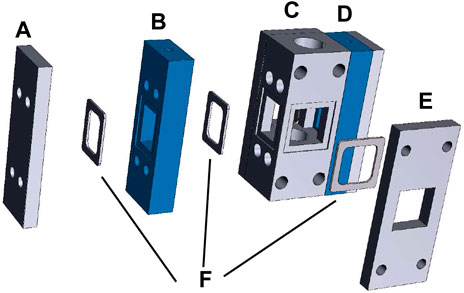
FIGURE 4. Testing vessel design. (A) Compression plate for anode compartment 1. (B) Anode compartment 1. (C) Cathode compartment. (D) Assembled anode compartment 2. (E) Compression plate for cathode compartment. (F) Gaskets and O-rings to form gas- and liquid-tight seals.

The milling machine, laser cutter, and 3D printer files for building the testing vessel are available on request.

Experimental Setup

The following components are required to assemble the testing vessel (Figures 5A–P):

1. The main body of cathode and anode compartments milled from polyether ether ketone (PEEK) plastic, assembled with threaded fittings and with glued (Epo-Tek 302-3M) PEEK tubing.

2. 3D-printed polylactic acid (PLA) compression plates for anodes, window, and cathode.

3. Silicone or Viton gaskets for sealing the photocathode and window.

4. Silicone or Viton O-rings for sealing between the anode, anode compartment, and membrane, and Nafion or other PEM.

5. 2–56 stainless steel screws for installing printed compression plates and hex wrench for assembly. Varying lengths needed depending on electrode and window thicknesses.

6. Fused silica or quartz window for front illumination, around 1.5 × 1.5 cm.

7. Two counter anodes with integrated electrical connections, no more than 1.2 cm wide, and two rectangles of Nafion approximately 0.5 × 1.2 cm.

8. Photocathode with ohmic contact and electrical connection, cut into 1.1 × 1.1 cm for a 1 cm² surface area that will be exposed to the electrolyte.

9. Reference electrode (Innovative Instruments 1 mm OD Ag/AgCl Ref Electrode) for three-electrode measurements or a sham RE made from sealed 1/16″ PEEK tubing if RE will not be needed.

10. Fittings for RE or sham RE assembly:

 a. IDEX M-650X Ferrules,

 b. IDEX M-644-03X flangeless nut,

 c. F-252 tubing sleeve for reference electrode (0.042″ ID × 1/16″ OD, for 1 mm OD tubing).

FIGURE 5

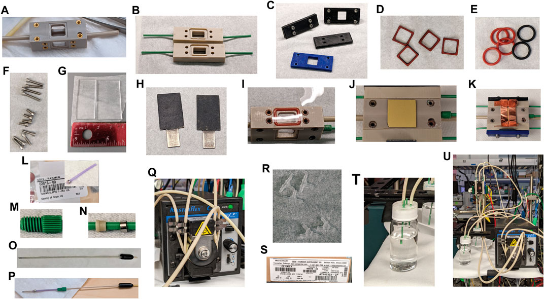
FIGURE 5. Components of the testing vessel. (A) PEEK cathode compartment. (B) PEEK anode compartments. (C) 3D-printed PLA compression plates. (D) Laser-cut silicone gaskets. (E) Size 013 silicone and Viton O-rings. (F) 2–56 stainless steel screws. (G) Quartz glass window. (H) Iridium oxide anodes with integrated electrical connection. (I) Nafion 115 cut to fit. (J) 1.1 cm square photocathode with a back ohmic contact. (K) An electrical connection, like copper tape, to the photocathode. (L) F-252 tubing sleeve for the reference electrode. (M) IDEX M-644-03X flangeless nut. (N) IDEX M-650X ferrules. (O) LF-1 Ag/AgCl reference electrode. (P) Complete reference electrode assembly. (Q) Masterflex peristaltic pump. (R) 1/16″ PVDF barbed “Y” or “T” fittings. (S) 1.42 mm ID PharMed BPT tubing. (T) Electrolyte reservoirs. (U) Assembled cell, pump, and reservoirs.

The following fluidics components are required for electrolyte circulation through the testing vessel during measurement (Figures 5Q–T):

1. A two-channel peristaltic pump (e.g., Masterflex from Cole Parmer), which provides the desired flow rate, approximately 5–10 ml/min.

2. Tubing: PharMed BPT, 1.42 mm ID, ColeParmer #95809-34.

3. 1/16″ polyvinylidene fluoride (PVDF) barbed “Y” or “T” fittings.

4. Anolyte and catholyte reservoirs. For this example, 2 × 20 ml glass scintillation vials were assembled with four pieces of 1/16″ PEEK tubing sealed into the caps with epoxy. One piece of tubing should extend into the vial far enough to draw up electrolyte from the bottom, while the other three should be short enough to not contact electrolyte when the measurement is running. An air-tight epoxy seal can be obtained by running a lip of tape around each cap to make a well, adding the four tubing pieces, then filling the well ∼1 mm deep with epoxy and allowing it to cure. One possible epoxy for this purpose is Epo-Tek 302-3M, used here. The “epoxy well” method of producing a thick epoxy layer produces a durable seal around the PEEK tubing, particularly when using corrosive electrolytes. An O-ring of appropriate size and material inside the cap is also required for an air-tight seal. One completed reservoir is shown in Figure 5T.

Parts should be cleaned before use: laser-cut gaskets should be sonicated in 10% nitric acid or soap and water prior to use. The leak-free reference electrode LF-1 should be stored assembled with the end submerged in 50 mM H₂SO₄. The quartz window should be cleaned with ethanol and dried with N₂. The Nafion PEM can be used dry (as-received) or soaked in electrolyte before assembly, with more difficult assembly with a soaked membrane but potentially also with quicker equilibration of the membrane and PEC cell through pre-hydration of the membrane.

Testing Vessel Assembly Procedure

The procedure is summarized in Figure 6:

1. Cut a piece of quartz glass or fused silica to 1.5 × 1.5 cm using the diamond scribe and running pliers. Place one of the square gaskets in the cell body on the side further from the RE inlet, and add the window (Figure 6A). Fix the front plate over a window with four screws, selecting screws long enough that there is even pressure on all sides, but avoiding bottoming out the screws, which may pull out threaded inserts and prevent sealing.

2. Using a diamond scribe dice the photocathode to ∼1.1 × ∼1.1 cm to fit the WE gasket (Figure 6B, inset).

3. If not already present, ohmic contact to the back should be made using the InGa eutectic alloy. Basically, for the material without preexisting ohmic contact, the steps discussed above for a photocathode without ohmic contact should be followed. The best process for the particular material should be determined by the experimenter. Care should be taken throughout this process to not generate uneven surfaces that will result in asymmetric pressures upon installation of the compression plate.

4. For photoelectrodes with an integrated ohmic contact as used here, InGa is not needed, and contact can be made by placing doubled conductive tape or other strong, pliable conductor on the back of the photoelectrode as in Figure 6B and holding it in place with the compression plate.

5. Place the second square gasket on the opposite side of the cell body, and add the prepared photocathode, followed by the second compression plate, arranging the electrical connector so it can be accessed from the long or short edge as desired. Add four screws of an appropriate length and tighten until just secured (Figure 6D). Overtightening the front and back plates can make them bend, eventually leading to electrolyte leaks, cracking a fragile sample, or pulling the threaded inserts out of the PEEK body.

6. Install O-rings in all six grooves of the anode compartments (Figure 6E). Viton O-rings can be used in contact with the counter electrode if transferring marks from silicone to the surface of the electrode is a concern. Use tweezers to add a piece of Nafion to one side (Figure 6F) and sandwich the Nafion with an anode compartment (Figure 6G). Add one anode and a compression plate with four long screws, and tighten the first anode compartment down (Figure 6H). To fully seat the O-rings and attain a good seal, tighten the screws until no gaps are visible between the main PEEK body and the PEEK anode compartment. Repeat to add the second anode.

7. Remove the RE assembly from the storage solution and screw it in firmly, or if not using a RE, the mockup/sham RE can be left installed between uses. Install the RE so that the tip extends into the chamber, as in Figure 6I. To prepare the RE or mockup for the first time, assemble components as illustrated in Figure 6J and screw them firmly into the RE port to set the ferrule and attain a permanent seal.

8. Attach tubing and a peristaltic pump between the cell and the electrolyte reservoirs and check for fluid leaks. See Figure 6K for suggested connections. The two CE chambers should be joined with Y- or T-connectors, or else three pump channels could be used. It is recommended that the cell be tested for electrolyte leaks with deionized water prior to adding an electrolyte to the reservoirs.

FIGURE 6

FIGURE 6. Assembly of the testing vessel. (A) Placing window. (B) Placing a placing a photoelectrode with integrated ohmic contact and folded copper tape for the connector. (C) Photoelectrode with ohmic contact added using InGa eutectic, silver epoxy, and copper tape. (D) Compression plate added to WE. (E) O-rings added to anode chambers. (F) Nafion added. (G) Anode chamber added. (H) Assembled with one anode compartment. (I) Depth for reference electrode in the cell. (J) RE and sham assembly. (K) Tubing connections and flow direction. (L) Pump, testing vessel, and reservoirs.

The use of this testing vessel for η_F and η_STH determination will be discussed below.

PEC Measurements

Light Source Calibration

Broadband measurements used to measure the saturation current level, onset potential, and STH efficiency are done under illumination by a solar simulator that mimics natural sunlight. The individual solar simulator to be used should be calibrated against the known spectrum of the sun prior to broadband current density-voltage (J-V) or η_STH measurements. The absorption losses due to the absorption of quartz windows and water electrolytes are negligible for most photoelectrodes. However, absorption in water becomes important for λ > 1000 nm for water film thicknesses of a typical PEC testing vessel (∼1 cm) and has to be accounted for smaller band gap absorbers and tandem absorber configurations (Döscher et al., 2014; Cendula et al., 2018; Moon et al., 2020). However, a PEC device in the field would experience similar UV/IR losses. Therefore, the reference spectrum and intensity should be calibrated at the front surface of the vessel to avoid errors that lead to artificially inflated performance values (Young et al., 2017). Additionally, careful calibration is needed for monochromatic light sources to accurately measure quantum efficiencies.

The output of the sun is attenuated by the atmosphere to varying degrees depending on the latitude on earth, because of the different angles of the incidence of sunlight. The angle of incidence governs the air mass (AM) that the light has to travel through. The standardized solar spectrum used for testing is the AM1.5 spectrum, illustrated in Figure 7. It is used as the reference spectrum for terrestrial solar testing because it corresponds to the sunlight reaching the ground through the average air mass above global mid-latitude locations. The AM1.5G (global) spectrum has a total irradiance of 1000 W/m² and includes both direct and diffuse radiation, where diffuse radiation encompasses reflected and scattered light and is roughly 10% of the AM1.5G irradiance. The AM1.5D (direct) spectrum does not provide the diffuse component, only the direct component, and has a total irradiance of about 900 W/m². Because AM1.5G is more representative of real-world conditions, it is the standard for most terrestrial solar applications.

FIGURE 7

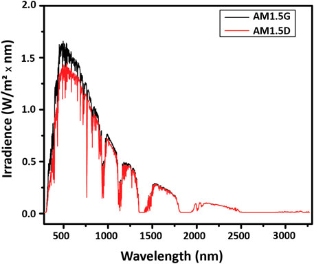
FIGURE 7. Terrestrial spectral irradiance. Available at https://www.nrel.gov/grid/solar-resource/spectra-am1.5.html.

Broadband Solar Simulator Calibration

Solar simulators vary in their ability to replicate the AM1.5G spectrum, and in general, their intensity may be adjusted to provide the correct total irradiance to the test device. The intensity adjustment can be done using a calibrated reference cell, ideally one with a band gap equal to that of the test cell. The reference cell used here consists of a Si photovoltaic cell with a calibrated short-circuit current value of 27.2 mA under the AM1.5G spectrum. The reference cell is calibrated separately (often by an external standards laboratory) to give the short-circuit current under a particular reference spectrum at a well-defined total irradiance.

The reference cell (RC) is placed at a set distance from the simulator, and its short-circuit current (I_sim,RC) is measured. Then, the irradiance falling on the reference cell is adjusted until the output current equals the calibration value. The irradiance is adjusted by moving the reference cell closer to or farther from the solar simulator. While the total irradiance can also be adjusted by varying the power going to the lamp, changing the current can change the spectral output of the lamp, so this is not recommended. The adjustment is complete when the measured short-circuit current from the reference cell equals the calibrated short-circuit current under the reference spectrum I_sim,RC:

$I_{sim,RC}=I_{ref,RC}=27.2mA.$

For this to be accurate, the band gap of the reference cell should match the band gap of the limiting junction of the photoabsorber under study. A Si reference cell will permit calibration for a Si photoabsorber, or another material with an equal band gap, to a reasonably high accuracy. However, a given photoabsorber that is studied may not have a band-gap-matched reference cell. In this situation, a reference cell of a different band gap may be used, with additional measurements made to compensate for the mismatch and accurately calibrate the solar simulator to deliver 1-sun illumination to the test cell.

Here, a Si reference cell with a band gap of 1.1 eV (1127 nm) is used to calibrate the total intensity of a xenon arc solar simulator to measure a GaInP test cell with a band gap of 1.8 eV (689 nm). In order to illustrate the issue that the mismatched band gaps can create, the spectrum of the lamp compared with the AM1.5G spectrum is shown in Figure 8. The total irradiance delivered to the Si reference cell corresponds to the integral from 1127 to 280 nm, and the total irradiance delivered to a GaInP test cell corresponds to the integral from 689 to 280 nm.

FIGURE 8

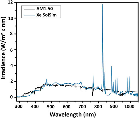
FIGURE 8. Spectral mismatch. The spectral shape of the lamp (Xe SolSim) differs from that of the reference spectrum, particularly due to the strong emission lines of Xe lamps around 800 nm. For accurate calibration, either a band gap-matched, calibrated reference cell or a spectral mismatch calculation is required.

Because of the strong emission lines from Xe lamps above 800 nm, by setting the intensity of the lamp using a Si reference cell such that there is the correct total irradiance below 1127 nm, the total irradiance for GaInP is too low. This means that if the total irradiance is calibrated without adjusting for the spectral mismatch, the photocurrent of the GaInP cell under reference conditions will be underestimated.

The solar simulator output is adjusted using a spectral mismatch factor M to address this issue (derivation in (Osterwald, 1986)):

${\text{I}}_{\text{sim},\text{RC}}=\frac{{\text{I}}_{\text{ref},\text{RC}}}{\text{M}}.(3)$

To calculate M, the spectrum of the solar simulator E_sim, the reference spectrum E_ref, and the spectral response of the reference and test cells, S_ref and S_test, must be known. The spectrum of the solar simulator can be found using an irradiance calibrated spectrometer, while the AM1.5G reference spectrum is widely available, for instance, from https://www.nrel.gov/grid/solar-resource/spectra-am1.5.html.

Spectral response is determined by measuring the quantum efficiency (QE) of the test and reference cells, which will be discussed more in later sections.

$M=\frac{{{\displaystyle \int }}_a^b{E}_{ref}\left(\lambda \right)\text{∗}{S}_{ref}\left(\lambda \right)d\lambda }{{{\displaystyle \int }}_a^b{E}_{sim}\left(\lambda \right)\text{∗}{S}_{ref}\left(\lambda \right)d\lambda }\text{∗}\frac{{{\displaystyle \int }}_a^b{E}_{sim}\left(\lambda \right)\text{∗}{S}_{test}\left(\lambda \right)d\lambda }{{{\displaystyle \int }}_a^b{E}_{ref}\left(\lambda \right)\text{∗}{S}_{test}\left(\lambda \right)d\lambda }.(4)$

The spectral response S(λ) is calculated from the QE by correcting for the relative energy of photons with different wavelengths:

$S\left(\lambda \right)\left(\frac{A}{W}\right)=\frac{q\lambda }{hc}\text{∗}QE\left(\lambda \right)\left(\frac{electrons}{photon}\right)=\frac{QE\left(\lambda \right)\text{∗}\lambda \left(nm\right)}{1239.8}.(5)$

The quantum efficiency and spectral response of the reference and test cells are shown in Figures 9A,B for this example. In Figure 9A, the Si and GaInP test cells absorb light between the UV limit and their respective band gaps.

FIGURE 9

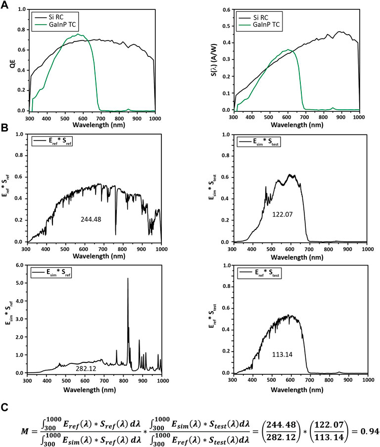
FIGURE 9. Calculating M for a Si reference cell (RC) and a GaInP test cell (TC). (A) Quantum efficiency and spectral response S(λ) from 300 to 1,000 nm. (B) Each product plotted against wavelength for calculating M, with the integral noted under the curve. (C) M is calculated to be 0.94 for this system, indicating the test cell should be moved closer to the solar simulator (vide infra). Specifically, the mismatch factor can be calculated with Eq. 4.

The spectral mismatch calculation is shown in Figure 9C. Numerical integration is done over the combined set of all wavelengths, with missing values filled in for each measurement by linear interpolation.

The details of the numerical methods during data collection and calculation can significantly affect the accuracy and precision of the calculated result. Because the various spectra were likely acquired at different sets of discrete wavelengths, it is necessary to interpolate the datasets to a common wavelength set for subsequent calculations. The best practice is to generate a single set of wavelengths that includes all of the various measurement wavelengths and then interpolate each spectrum to that common set. This scheme thereby preserves all of the original measurement information. The next-best option is to use the most granular of the individual datasets as the common wavelength set. For example, if the AM1.5G reference spectrum is measured every 0.5 nm but the spectral response is measured only every 10 nm, interpolate the spectral response data to the reference spectra wavelengths to generate the additional values.

In one suggested method for accomplishing this in an automated fashion, each spectrum can be imported into a Pandas dataframe in Python, followed by concatenation of the spectral response, solar simulator spectrum, and AM1.5G spectrum dataframes, and sorting by the wavelength column, for example:

df_all_list = [df_SR, df_sol_sim, df_am1pt5]

df_all = pd.concat(df_all_list, ignore_index = True)

df_all.sort_values(by = “nm”, ascending = True, inplace = True)

Linear interpolation may then be done (a simple method uses Excel), followed by numerical integration and calculation of M.

Once the mismatch parameter is obtained, the absolute irradiance of the solar simulator can be set using the reference cell to complete calibration.

$I_{sim,RC}=\frac{I_{ref,RC}}{M}=\frac{27.2mA}{0.94}=28.9mA.(6)$

Additional information on this calculation, modifying the solar simulator spectrum by adding light emitting diodes (LEDs) to increase the intensity at specific wavelengths, and application to multijunction cells can be found in the literature (Osterwald, 1986; Moriarty et al., 2012). Note that the spectral mismatch M should be considered a correction factor rather than a random error. Failing to account for the mismatch systematically reduces the accuracy of the measurement by changing the irradiance. It does not simply increase the uncertainty of the measurement. A full treatment of the problems associated with large values of M is beyond the scope of this protocol.

For a multijunction material consisting of components with different light absorption properties, it may be difficult to set the absolute irradiance to satisfy all constituent cells with a given solar simulator. In general, one needs adjustable LEDs or narrow-band light sources and separate reference cells for each junction in the multijunction cell. If those features are not available, the irradiance should be set to provide 1 sun to the current-limiting junction, which can usually be determined from the QE or incident photon to current efficiency (IPCE) (below). This should be noted in the publication. In the example here, GaInP is the current-limiting junction, so the light source calibration was done to deliver 1 sun to that junction. It is also a good idea to estimate the irradiance to the other junctions using the spectral mismatch procedure described above to make sure that the assumed non-limiting junctions are, in fact, not limiting.

Monochromatic Light Source Calibration

Measuring QE for the reference and test cell in the previous section requires a monochromatic light source, typically consisting of a white light source combined with a monochromator. For determining QE, the photocurrent is measured as the wavelength is scanned; then, the photocurrent at each wavelength is normalized by the monochromatic light output. The light output is measured at each session using a photodiode (PD) of a known (calibrated) QE. Photodiodes with measured, NIST-traceable QE can be obtained from Thorlabs (e.g., ThorLabs FDS1010-CAL) or other vendors, or any other stable photodiodes can be calibrated using a spectrometer. The calibration data of the photodiodes are typically collected at short circuit, and they should be measured at short circuit here as well. The band gap of the PD has to be equal to or lower than the band gap of the investigated material.

The simplest method to find the monochromatic light power is to use a photodiode with an up-to-date factory calibration of spectral responsivity. Herein, a ThorLabs FDS1010-CAL photodiode was used to determine the output of the monochromator by measuring the photocurrent output at each wavelength and dividing by the value of the spectral responsivity at that wavelength (Figure 10A).

FIGURE 10

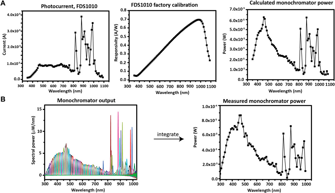
FIGURE 10. Photodiode application and calibration. (A) Using a calibrated photodiode to measure monochromator output. (B) Measuring the monochromator output with a spectrometer in order to calibrate a photodiode.

To calibrate a photodiode which was not factory calibrated, the monochromator power can be measured with a spectrometer; then, the responsivity plot can be generated from the ratio—at each wavelength—between the photodiode current and the measured power. In Figure 10B, the measured spectrum of each monochromatic wavelength of interest (300–1010 nm, in increments of 10 nm) is shown overlaid. The spectra were measured with an OceanOptics HR+C2276 spectrometer with a cosine corrector. The total optical power at each wavelength of the monochromator is found by integrating each spectrum. After the power spectrum is obtained, it can be used to calculate the responsivity curve of the photodiode that will be used during IPCE. Note a slight difference in scale between the measured and calculated monochromator power due to a different spot size used for the two photodiode measurements. However, the spot size will not affect the IPCE measurement because an underfill spot (only a fraction of the active area is illuminated) is used on the photodiode and sample at each measurement.

Monochromatic Photocurrent Measurement via Incident Photon-to-Current Efficiency

The photocurrent under a monochromatic light source is used to determine the spectral response of a PEC cell. QE—the efficiency with which photons are absorbed and converted into mobile electrons (i.e., current)—is a key measurement for PEC materials, just as it is important for characterizing photovoltaic (PV) materials. QE is also needed to calculate the spectral mismatch factor for light source calibration as in the previous section. For PEC, QE is measured by IPCE, where the photocurrent, as a function of wavelength, is determined for the photoelectrode. The wavelength of a monochromator is scanned while the short-circuit current is recorded, and the current is normalized to the light flux from the monochromatic source. The IPCE shows values between 0 and 1 in the region of the spectrum where the photoabsorber is sensitive. IPCE is generally a direct current measurement, in contrast to the QE measurement of solar cells, which is typically an alternating current measurement done with chopped monochromatic light and a lock-in amplifier.

Experimental Setup

Equipment:

1. Photoelectrodes prepared as above from 5 mm square samples.

2. Potentiostat.

3. IPCE testing vessel, that is, an electrochemical cell with optical glass/other optically transparent windows.

4. Counter electrode.

5. Reference electrode (if a bias must be applied to split water).

6. Broadband light source, monochromator, and second-order/order-sorting filters.

7. Bias light source(s), for example, high-power LEDs.

8. Calibrated photodiode.

9. Measurement automation, for example LabVIEW, to control the monochromator and potentiostat throughout the wavelength sweep, and control the shutter for measuring dark and light current.

Two examples of IPCE setups are shown in Figure 11, with components labeled, but other arrangements are possible.

FIGURE 11

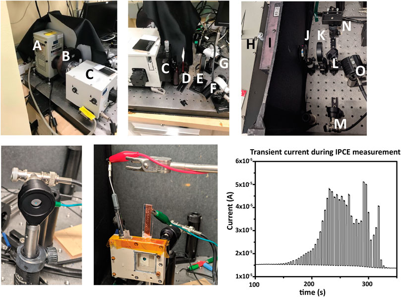
FIGURE 11. IPCE measurement. Top row, two examples of instrumentational setup. (A) a Xe arc lamp, (B) computer-controlled shutter for generating light/dark conditions, (C,H) monochromators, (D,I) second-order filter(s) (E,K) lenses to focus monochromatic light to an underfilled spot on the sample, (F,O) high-power LEDs for applying bias light, and (G,N) the sample locations. Also shown is the option of using a mirror (L) to alternate directing the monochromatic light from the PD (M) and the sample (N). An iris (J) can restrict or increase the total light intensity if needed. A dark box or enclosure surrounding the light path from the monochromator aperture to the sample is required to eliminate stray light from the measurement. Bottom row: at the start of each IPCE measurement, the photodiode current is measured to determine monochromator spectral output for the underfill spot. The underfilled spot is then aligned to the photoelectrode in the electrochemical cell, and bias lights and any electrical bias are set. Chronoamperometry is then measured simultaneously with the wavelength scan. Light and dark measurements can be shown during acquisition in the form of a transient photocurrent graph.

Because the photocurrents measured during IPCE are relatively small, a dark box/enclosure must be used to enclose the entire optical path to eliminate interference from stray light.

Different experimental setups with respect to the electrical and light bias applied should be used depending on the type of the analyzed photocathode.

In all cases, the monochromatic light should fall fully within the photoelectrode active surface area and the active surface area of the calibrated photodiode. This is referred to below as forming an “underfill spot” on the photoelectrode/photodiode and is required to obtain meaningful results from an IPCE measurement.

For photocathodes that spontaneously split water, a two-electrode setup is used, with 0 V bias applied between the WE and CE. The CE should be a high-quality OER catalyst such as IrO_x. Report the CE and any other conditions used along with the IPCE.

For photocathodes that do not spontaneously split water, in order to apply a controlled bias during the measurement to attain water splitting, a three-electrode setup is used. The required bias is applied between the WE and RE as the wavelength is scanned and the photocurrent monitored. It is good practice to report these conditions along with the IPCE results.

In addition to an electrical bias, a light bias is often used, for instance, through illuminating the sample with a high-power LED.

For single-junction photoelectrodes, a white light bias is often needed. A high-power LED such as a 1,000 mA Mightex fiber-coupled LED light source, outputting up to around 10 mW of illumination, can be used. A bias light is needed because the flux from the monochromator is typically much lower than that of an AM1.5G source in a given wavelength range, and additional illumination is needed to increase the signal/noise ratio of the photocurrent and fill trap states that would otherwise interfere with the measurement by artificially inflating the onset potential. The power of the bias light is set so that the photocurrent with the bias light, plus any electrical bias, is around 37% of the saturation photocurrent for the device (Chen et al., 2013), with adjustments made as needed after initial data are acquired.

For tandem or multijunction photoelectrodes, the total device photocurrent is that of the current-limiting junction (we neglect luminescent coupling effects here (Steiner et al., 2012). Thus, to measure the IPCE of each junction individually, the other junction is illuminated with a bias light of an appropriate wavelength. The intensity of the bias light is set high enough to saturate the second cell and make the first the current-limiting junction (and vice versa) so that the measured current from the PEC cell will correspond only to the photocurrent of the investigated junction. For the GaInP/GaAs tandem junction photoelectrode discussed in this study, a 470 nm LED bias light is used to saturate the GaInP cell while measuring IPCE of the GaAs subcell, and an 850 nm LED bias light is used to saturate the GaAs cell while measuring the IPCE of GaInP.

The flux of the LED should typically be several times that of the flux from the monochromatic source to ensure that the measured subcell is current-limiting at all wavelengths. To prevent issues resulting from this, the experimenter should make sure no features from the monochromator are observed in the IPCE measurement. For example, a Xe-based monochromatic light source will have several very large emission peaks in the IR. If corresponding features are observed in the IPCE measurement of the GaAs subcell of GaInP/GaAs, the bias light intensity to the GaInP subcell is not sufficiently high. Another way to assure high enough bias light intensity is with a calibrated photodiode or irradiance calibrated spectrometer. For example, the 470 nm LED was set to 0.3 A to attain power from the LED of 1 mW after it was determined that the monochromator had around 400 µW reaching the GaInP cell.

For the GaInP/GaAs tandem photocathode, with a 1.8 eV/689 nm GaInP top junction and 1.4 eV/886 nm GaAs bottom junction, water is split at 0 V applied bias under an AM1.5G illumination source, so no electrical bias is used. As a multijunction photocathode, in order to measure the IPCE of the top GaInP cell, the bottom cell is illuminated with a high-power 850 nm LED while the monochromatic response of the cell as a whole is scanned. The infrared light causes excitation of the smaller band gap GaAs only, rendering the larger band gap GaInP current-limiting. To measure the IPCE of the bottom GaAs cell, the top cell is illuminated with a high-power 470 nm LED while the short-circuit current of the cell is measured (Young et al., 2017). The measured IPCE for this photocathode from 300 to 1000 nm is shown in Figure 12A.

FIGURE 12

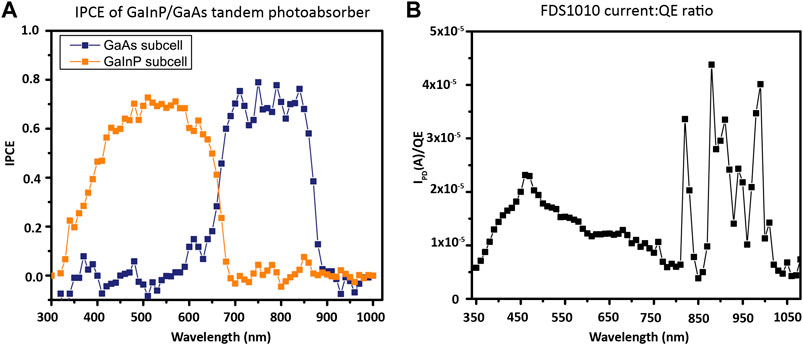
FIGURE 12. IPCE calculation. (A) Two-electrode, 0 V bias, IPCE of GaInP/GaAs photocathode, acquired with 1 mW bias light illuminating the junction not being measured. (B) Calibrated photodiode photocurrent:QE ratio. Because the calibration of FDS1010 is done from 350 to 1050 nm, the x-axis between the two samples differs slightly.

A range of different electrochemical cell architectures can be used as a testing vessel for measuring IPCE, so long as an optically transparent window is present. Compression cells allow for easy sample mounting and make it possible to expose an identical surface area for each sample. On the other hand, as shown in Figure 11, a cuvette cell allows for rapid WE exchange and typically more flexibility in WE dimensions and in the used type of CE and/or RE. Here, we used a cuvette cell for characterization.

The IPCE spot size is also important. An underfill spot, where the monochromatic light spot is fully contained in the photodiode and WE surface area, is used for IPCE measurements. This means total irradiance is used in determining IPCE rather than spectral power density over the spot area. This is done to remove errors resulting from the relative concentration of the monochromatic spot in the PEC cell compared to the photodiode. Because all solar simulators have a diverging beam and J-V measurements are generally conducted with illumination overfilling the active area, the light is concentrated when passing through the air/glass/electrolyte interfaces of PEC cells (Döscher et al., 2016). This error is generally 10% or more for top-of-the-line commercial solar simulators but also depends on sample area and light pathlength through the electrolyte. Because the amount of concentration in the PEC cell compared to the photodiode (which has no electrolyte-caused concentration of light) is unknown, using an overfill spot will introduce a potentially large error into the experiment and should be avoided. Thus, IPCE measurements are performed with a spot size smaller than the active area of the sample (i.e., underfill illumination, with examples seen on both the photodiode and the WE in Figure 11) to serve as a validation measurement that is active-area independent and absent of the PEC cell concentration error. Focusing the light to an underfill spot for both the sample and the calibration photodiode also simplifies the calculation of IPCE, which would otherwise require measurement of the illuminated region of the sample and the photodiode.

Procedure

Because the output of the monochromator will vary as the lamp ages, the light output must be measured with the photodiode at a minimum at the start of each IPCE session, following lamp warmup. Most lamps require about 20 min of operation before the time-stable output is achieved, so this should be done before beginning measurements.

1. Turn on the lamp 20+ min before starting a measurement.

2. As lamp warms up, set up the PEC cell with the WE, CE, and optionally RE in the IPCE testing vessel. Confirm that the WE surface is fully immersed in the electrolyte solution.

3. The monochromator spot can also be aligned during the warm-up period. Set the monochromator to 550 nm, and focus the light to make an underfilled spot (light falls fully within the active area) on the photodiode (PD). Then, replace the PD with the assembled PEC cell, and adjust the location of the electrodes and cell so that the monochromatic light forms an underfill spot on the center of the WE. If needed, adjust the lens, iris, and/or mirror locations, distances, and angles to obtain a focused underfill spot on both the PD and WE when one is simply switched for the other without adjusting optical angles. It is important not to inadvertently alter the light path between the PD measurement and the sample measurements.

4. Select a wavelength range over which to measure based on the expected band gap(s). A shutter should be employed to permit measuring light and dark current at each wavelength.

• Non-ideal photoelectrodes that exhibit transient, capacitive current should allow sufficient time at each wavelength for the photocurrent to stabilize. Otherwise, the IPCE data will be inflated. Typical stabilization times can be several seconds or longer and chopping frequencies of 1 Hz or faster generally lead to error—hence a shutter is preferred to a chopper as the switching frequencies should be set to 0.2 Hz or slower to allow any capacitive currents to settle out.

5. To identify the suitable potential for IPCE measurements, for photoelectrodes that do not split water at zero bias, broadband J-V and/or chronoamperometry (CA) measurements should be carried out in a three-electrode setup. Generally, the bias may be selected based on the desired current density.

• A direct translation between performance under 1-sun broadband and that of IPCE measurements is generally not expected. Because IPCE is measured at low light flux (uA), the kinetic overpotentials are lower than under broadband illumination (mA) and thus, this loss channel may not be accounted for in the IPCE measurement. For this reason, the integrated IPCE measurement should be considered the best-case, upper limit of photocurrent under broadband illumination.

6. Using the calibrated photodiode, measure the short-circuit current at each wavelength in the desired range with the chosen step size (typically 5–10 nm, but restricted by the peak width of the monochromatic light at each wavelength). During this measurement, the positioning should ensure that all of the monochromatic light is focused within the photodiode active area, and the photodiode should not be placed in a filled/empty beaker or any other “simulated” PEC condition. Dark current should be avoided or subtracted out using dark current measurements.

7. Following photodiode measurement, direct the monochromatic beam to an underfill spot on the photoelectrode in the PEC cell, turn on the bias light if needed, start the zero-bias or applied-bias CA measurement, and begin the monochromatic light sweep.

• An example of an automation sequence that may be done in LabVIEW or other available software: the monochromator moves to a new wavelength, the shutter opens, potentiostat continuously records current, photocurrent is allowed to stabilize, a period of data points after stabilization is averaged, the shutter closes, potentiostat continues to record current, the current is allowed to stabilize, and a period of dark current data points after stabilization is averaged. If automation is not possible with available equipment, stepping the monochromator in a single step from a long wavelength corresponding to sub-band-gap photon energies to a short wavelength characterized by above-band-gap photon energy at the start of the sweep will create an instantaneous capacitance current that can be read in the measured current to identify the time at which the sweep began.

Other experimental considerations are presented below.

Luminescent coupling of multi-junction cells, where radiative recombination of carriers in one junction generates additional photocurrent in a neighboring junction, can lead to non-linear response as a function of the broadband light intensity. To determine if there is concern that this is a factor for the multijunction cell used, we can perform measurements at several bias light intensities for junctions other than the top junction and assess the linearity of response (Steiner and Geisz, 2012).

If reaction kinetics are limiting, a comparison of measurements with and without a facile redox couple could be used. If a redox couple is used that has absorption features overlapping with those of the measured photoelectrode, the electrolyte solution should be prepared with a low enough concentration of the redox couple to ensure that parasitic light absorption by the couple is minimized. Alternately, the absorption coefficients of the redox couple, combined with the known path length of the cell, can be used to correct the irradiance of the incident light to account for absorption by the redox couple. The presence of a redox couple should be reported along with the data.

Calculating IPCE

The QE of the calibrated photodiode is easily determined from its spectral responsivity (with an example of the factory calibration shown in the center panel of Figure 10A). From the QE of the photodiode (QE_PD) and the photocurrents of the photodiode and the photoelectrode (I_PD and I_PEC, respectively), the photoelectrode sample IPCE (QE_PEC) can be calculated by setting equal the ratios of the photocurrent/QE:

$\frac{{\text{I}}_{\text{PEC}}}{{\text{QE}}_{\text{PEC}}}=\frac{{\text{I}}_{\text{PD}}}{{\text{QE}}_{\text{PD}}}.(7)$

Therefore, at each wavelength, IPCE should be calculated as I_PEC divided by I_PD/QE_PD (Figure 12). Prior to this calculation, the measured dark current should be subtracted from the measured current under illumination to obtain the photocurrent for each wavelength.

Broadband Photocurrent Measurement

The broadband photocurrent is measured under a solar simulator spanning all the wavelengths present in the AM1.5G spectrum. The photocurrent is a function not only of the photoelectrode but also of the specifics of the PEC cell setup, including the presence of a membrane and the electrolyte, and whether it is a two- or three-electrode configuration. In the case of a two-electrode configuration, the properties of the counter electrode are important. Therefore, each of these details should be reported precisely in publications and kept constant between measurements of a particular photoelectrode material. In addition, testing vessels for PEC water splitting may have various shapes and configurations that can affect the iR drop in the photoelectrochemical system. High concentrations of the electrolyte can help mitigate this issue.

Two broadband measurements will be discussed here. First, linear sweep voltammetry (LSV) can measure current J-V characteristics of the photoelectrode under the calibrated broadband source and provide photocurrent onset potential and current density at the desired operating potential. Second, the photocurrent can be measured over a period of time, designed to mimic operational conditions to track stability (chronoamperometry). The J-V characteristics of the cell prior to, during, and following the stability test can be used to understand changes in the performance of the photoelectrode and cell over time. Additionally, the measurement of the potential required to maintain a constant current (chronopotentiometry) can also provide information on the stability of the photoelectrode. Photoelectrode corrosion products can be tracked by inductively coupled plasma mass spectrometry (ICP-MS) of the used electrolyte and X-ray photoelectron spectroscopy (XPS) of the photoelectrode following completion of the durability test, although describing these measurements is outside the scope of this work.

LSV is used to measure the J-V characteristics of a PEC cell. The saturation current density, expressed in mA per cm² of electrode surface area, is a key metric for determining η_STH of a material. Onset potential determines if a PEC cell will generate enough photovoltage to operate bias-free. Figures 13A,B show a characteristic J-V curve when applying a bias negative of the onset of photocurrent in two- and three-electrode configurations.

FIGURE 13

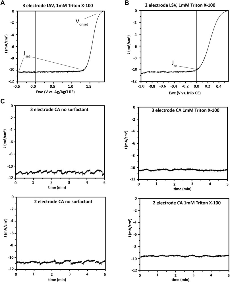
FIGURE 13. Broadband PEC characterization. (A), three-electrode and (B), two-electrode linear sweep voltammetry (LSV or J-V) showing onset potential, saturation current density, and short-circuit current density for a III–V photoelectrode, in 0.5 M H₂SO₄ with 1 mM Triton X-100 surfactant. (C), Photocurrent at 1-sun illumination and 0 V applied potential for a III–V photoelectrode. A comparison is made between two- and three-electrode bias free water splitting, and another between electrolyte with and without 1 mM Triton X-100 as surfactant effects on bias free water splitting. The electrode is seen to have similar currents in two- and three-electrode formats, with less variation in current over time when surfactant was used in the electrolyte. Surfactants such as Triton X-100 decrease the size of hydrogen bubbles formed, which prevents formation of large bubbles blocking portions of the photoelectrode. However, surfactant may decrease the average current, as seen here, while providing less variation over time by eliminating large bubbles.

CA is used to determine photoelectrode stability. In CA, the operation potential of the cell—0 V for a bias-free water-splitting material in a two-electrode configuration, or a non-zero applied potential in a three-electrode configuration if a bias is needed—is applied and the current is measured as a function of time under illumination. Alternatively, with chronopotentiometry (CP), a specific current density is maintained in the cell by altering the potential applied, and the applied potential is tracked. CA is often chosen for measuring the stability of photoelectrodes. In contrast, CP may be chosen to monitor the stability of stand-alone catalyst layers to determine how long the current density of interest can be driven through them before they fail. Prior to CP or CA, LSV is done and the operating point is selected (0 V in the case of the example here, as shown by the J_sc point in Figure 13B).

Following the stability test (1, 10, or 100 h, etc.), another LSV is done to monitor degradation in performance. During longer stability tests, it is common to stop the CP or CA periodically, for instance, every hour, and collect additional LSV so that changes in the J-V characteristics can be recorded over time. For example, recently, the J-V characteristics of a GaN/Si photocathode were tracked every 1–2 h over a 10 h CA measurement, and it was seen that the largest change in onset potential occurred during the first hour (Zeng et al., 2021).

Figure 13 illustrates the difference that surfactant in the electrolyte makes in the current profile of a CA measurement with 0 V applied bias. A surfactant lowers surface tension and encourages the formation of small bubbles, which are easily released from the photocathode surface. Large bubbles that form without a surfactant block part of the photocathode surface from light and electrolyte. This effect reduces the current until the bubble releases from the surface and generates a periodic fluctuation of the photocurrent.

Both two- and three-electrode measurements are useful for broadband measurements of a new PEC material.

In a three-electrode measurement, a known potential is applied between the WE and RE, and the properties of the WE are determined. In this measurement, the potential is dropped solely between the RE and the WE, and the potential of the RE remains essentially constant under small applied potentials. Therefore, sensitive measurement of the properties of the working photoelectrode in the specific cell and electrolyte can be made. In this case, the potential required to drive the hydrogen evolution reaction for a given photocathode can be determined independently of the CE reactions.

In a two-electrode measurement, on the contrary, the potential is applied between the WE and CE, and because the counter electrode has an unknown and undefined potential in the system, the onset potential measured in a two-electrode setup is the potential required for that system, with no independent values calculable for the photocathode specifically. Because of this difference, two-electrode properties such as η_STH of an integrated photoelectrode cannot be extrapolated from data collected in a three-electrode setup. In contrast, materials that do not split water at zero bias may still be quantified as to the amount of hydrogen produced. A three-electrode setup is used for this case, and a potential is applied between the RE and WE to provide the voltage needed for water splitting. However, these conditions must be reported, and the values obtained cannot be compared with two-electrode short-circuit water-splitting efficiencies since that attempts to replicate conditions that will be suitable to use in the field.

Two-electrode measurements are vital for demonstrating bias-free water splitting and quantifying η_STH because they mimic the real-world conditions of a PEC water-splitting device with only sunlight as an input. For example, Figure 13 shows the two-electrode J-V and durability measurements for a GaInP/GaAs photocathode and an IrO_x anode. The J-V measurement illustrates that the material will perform bias-free water splitting, while the CA shows a slow decrease in photocurrent over the first hour of bias-free water splitting.

Experimental Setup

Equipment and supplies for broadband measurements:

1. Photoelectrode(s) as the working electrode.

2. Potentiostat.

3. Testing vessel (can be the same used for IPCE).

4. Counter electrode.

5. Reference electrode.

6. Broadband light source.

The PEC cell should be set up the same way as IPCE, except that a reference electrode is needed to obtain three-electrode measurements, irrespective of if the photocathode splits water at 0 V applied bias. Three-electrode measurements allow the characterization of the new PEC material alone, independent of the CE, and can be informative for material development.

Procedure

J-V analysis:

1. Prior to a measurement, warm up the lamp for 20+ min with the shutter closed. During that time, set up the PEC cell in a three-electrode format (WE, CE, and RE, each clipped to the appropriate potentiostat lead). The WE should be fully immersed, and at least, an equal area of the CE should also be immersed in the electrolyte.

2. Set the potentiostat to perform LSV in the region of interest. For cathodic currents for HER, with the photocathode as the WE, the potential should scan from negative values to the open-circuit voltage (V_oc). If anodic currents are known to damage the photocathode, it is important to stop the scan before the current crosses the x-axis (i.e., becomes positive) and to scan from negative values toward V_oc, which prevents a small anodic current from being drawn through variation of the V_oc between the initial measurement and the start of the LSV scan. Input the surface area of the WE measured previously into the potentiostat software. The scan rate should be set to no more than 10–20 mV/s to avoid non-Faradaic current contributions that artificially inflate measured current values. The potential range and scan rate should both be reported when publishing.

3. With the shutter still closed, perform an LSV scan in the dark to confirm there is minimal dark current. Then, open the shutter and collect an illuminated LSV scan. Alternatively, a single scan where the light is chopped every other 100 mV can collect dark and illuminated responses in a single run, but illumination should not be blocked within a few 100 mV of V_oc.

4. Unclip the potentiostat lead from the RE in the PEC cell, and clip it onto the CE to short the potentiostat RE and CE leads. Run a two-electrode LSV.

5. Finally, replace the RE lead and run a second three-electrode LSV. This can later be used for a comparison with the first scan.

6. Repeat the 3-2-3 series of measurements with additional photoelectrodes.

Stability:

1. Prior to a stability test, measure dark and light LSV in the same format (two- vs. three-electrode) as is planned for the stability test.

2. Set up the potentiostat for CA with a constant voltage (can be 0 V) applied. It can also be set up to periodically measure LSV, for example, alternating 1 h of CA with an LSV measurement. One important consideration is the total length of the file—if many hours or days of data will be collected, it is best to collect a data point only once per second or once per 5 s. Otherwise, it is possible to produce unmanageably large files.

3. Run the CA.

Data

In the software of your choice, divide the current from the potentiostat in mA by the measured area in cm² before plotting LSV, CA, or CP. See above for surface area measurement. Some potentiostat software may permit exporting data in terms of current density if the surface area is entered into the experimental parameters, and most software will show a plot of current density as the experiment is running if the surface area has been entered as a parameter.

Record the saturation current density and the onset potential for each LSV. We find that the definition of onset potential for a photoelectrochemical reaction may have different descriptions across the field (Zou and Zhang, 2015). It is sometimes defined by the potential at which the current density reaches a certain value, for instance, 1–10 mA/cm², or as the potential at the intersection of a line fit to the squared photocurrent in the region near the onset potential of the LSV with the voltage axis (Chen et al., 2013). When reporting results, state clearly how the onset potential is defined for your system, along with reporting its values.

Measurement of Faradaic Efficiency and Solar-to-Hydrogen Efficiency

The Faradaic efficiency η_F, is the efficiency with which electrical current is converted into hydrogen and oxygen in an electrochemical cell; see Eq. 8. Hydrogen consumes two electrons per molecule H₂ produced, while oxygen produces four electrons per O₂ molecule produced.

${\text{η}}_{\text{F},\text{ H}2}=\frac{\left({\text{H}}_2\text{produced}\right)}{\left(\text{measured current}\right)}=\frac{\left(\frac{\text{mol}}{\text{s}}{\text{H}}_2\text{∗}\frac{2{\text{e}}^{-}}{{\text{H}}_2}\text{∗F}\left(\frac{\text{C}}{\text{mol}}\right)\right)}{\text{I }\left(\text{A}\right)}$

${\text{η}}_{\text{F},\text{ O}2}=\frac{\left({\text{O}}_2\text{produced}\right)}{\left(\text{measured current}\right)}=\frac{\left(\frac{\text{mol}}{\text{s}}{\text{O}}_2\text{∗}\frac{4{\text{e}}^{-}}{{\text{O}}_2}\text{∗F}\left(\frac{\text{C}}{\text{mol}}\right)\right)}{\text{I }\left(\text{A}\right)}.(8)$

This is equivalent to the fraction of current measured in the PEC circuit consumed in the water reduction and oxidation half-reactions, not considering product losses. A less than 100% η_F indicates competing electrochemical reactions, recombination of products prior to collection, loss of products prior to measurement, and/or membrane crossover in the testing vessel.

STH efficiency or η_STH is the efficiency with which incident sunlight is turned into hydrogen (and oxygen).

η_STH can be calculated by first measuring η_F and then using Eq. 1 (repeated) here:

${\text{η}}_{\text{STH}}=\frac{{\text{j}}_{\text{sc}}\left(\frac{\text{mA}}{{\text{cm}}^2}\right)\text{∗}1.23{\text{V∗ η}}_{\text{F}}}{{\text{P}}_{\text{total}}\left(\frac{\text{mW}}{{\text{cm}}^2}\right)}.$

In this equation, J_sc is the short-circuit current density from a two-electrode measurement (not from a three-electrode measurement). The amount of H₂ produced is best measured with a GC, though volumetric methods (i.e., the Hofmann apparatus used by Chen et al. (2011)) can also be used if corrected using the vapor pressure of water at the collection temperature. While the evolved gas can be quantified by GC either by periodically sampling with a syringe or using a continuous purge of carrier gas, the latter method is preferred because sampling with a syringe may be subjected to sample contamination with air (Wang et al., 2021). Therefore, a closed electrolyte loop and a closed carrier gas channel loop through the electrolyte reservoir’s head space is used in this protocol as a demonstration.

For determining η_F, a two-electrode CA at 0 V WE/CE bias under 1-sun illumination is run, and the amount of H₂ produced is measured. The sealed compression cell presented above can be used as the testing vessel for this purpose, as done here for GaInP/GaAs. For materials that do not split water at zero bias, a three-electrode CA can be done with a voltage applied between the WE and RE, but this alternative setup must be clearly stated in reporting results, and the results cannot be extrapolated to indicate η_STH of the photoelectrode.

Experimental Setup

Required equipment:

1. Sealed compression cell described above.

2. Gas-tight electrolyte reservoirs and tubing connections.

3. Gas-tight traps to prevent liquid from entering the GC.

4. WE and CE of appropriate form factors for compression cell.

5. Reference electrode (if a bias must be applied to split water).

6. GC.

7. Broadband light source.

8. Computer hardware and software such that timestamps can be synchronized between CA and GC output data to correlate changes in products with changes in current. The log files of mass flow meters may be used to quantify product streams for accurate η_F/η_STH calculation.

The specifics of GC operation will differ depending on the system, and we provide here an overview of the process of η_F measurement using an Agilent GC. Adjustments should be made based on the equipment available. Figure 14 details the experimental setup used here with the above equipment.

FIGURE 14

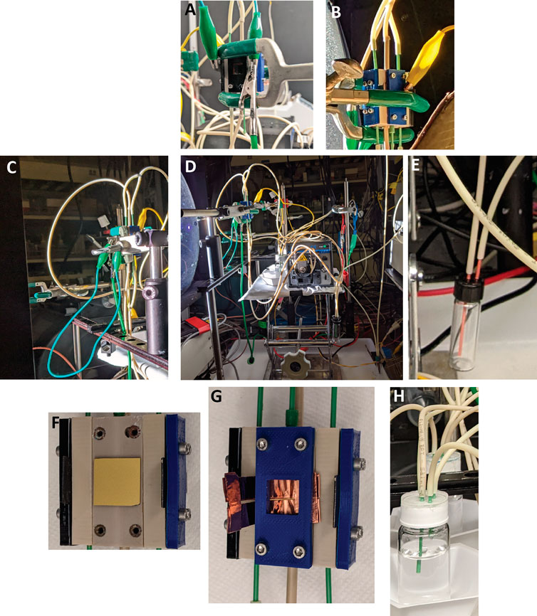
FIGURE 14. Schematic of η_F measurement. (A) Anode connections to potentiostat. (B) Photocathode connection to potentiostat. (C) Testing vessel clamped at a distance of 1-sun from the solar simulator. (D) Test vessel setup: solar simulator on left, electrolyte pump, and reservoirs in the center, and GC traps leading to the GC on the right. (E) A liquid trap placed between the electrolyte reservoir head space and the GC to prevent liquid from being drawn into the GC. (F) Photocathode. (G) Electrical connection for photocathode and compression plate. (H) Two electrolyte reservoirs with carrier gas inlets and outlets connected to the GC traps, in addition to the electrolyte circulation inlet and outlet.

An inert gas, N₂ or Ar, is used as a carrier gas flowing through the head space of both electrolyte reservoirs. It is beneficial to measure both H₂ and O₂ production to confirm no leaks in the system (see data analysis section) and detect possible corrosion reactions (Kistler et al., 2019). Therefore, the head space of both anolyte and catholyte reservoirs should be sampled. The carrier gas flow rate should be chosen accordingly to place the concentration of H₂ and O₂ within the calibration range of the GC and speed up the equilibration of the system and GC readings. Greater flow rates have the benefit of resulting in quicker measurement of the generated H₂ because it is pushed faster from the reservoir head space to the GC. However, a too high flow rate will decrease the signal-to-noise ratio of the GC peaks. In extreme cases, it can also dilute the H₂ beyond the limit of detection of the GC, so some experimentation may be required to find the optimal flow rate. Faster equilibration may be obtained by first flushing the electrolyte reservoir headspaces with carrier gas for 20 min before beginning the experiment. The choice of the carrier gas can be determined by the location of the N₂ peak in the particular GC spectrum. If it overlaps with the peak of interest, Ar can be used instead.

Prior to measurement, the GC should be calibrated by delivering a series of known concentrations of H₂ and O₂ using calibrated flow controllers/meters, ideally at the flow rate used in the η_F measurement.

Warm up the calibrated solar simulator for 20+ min before taking any measurements. The flow rates of carrier gas are ideally controlled programmatically, for example, by LabVIEW.

1. Testing vessel setup:

a. Assemble the compression cell, including WE, CE, and optional RE, and attach anode and cathode chambers to the electrolyte reservoirs with tubing. Circulate the electrolyte with a previously calibrated peristaltic pump. The flow rate used for the examples here is 10 ml/min.

i. Clamp the cell such that the photoelectrode is in the plane of the 1-sun calibration for the solar simulator.

2. Mass flow controller (MFC) setup:

a. Typically, the inlet of the carrier gas will be controlled by one MFC, and a mass flow meter (MFM) will measure the flow rate at the outlet of the GC column. Confirm that the correct gas (N₂ or Ar) is selected on each MFC and MFM.

b. Set the flow rate of the carrier gas to 1 SCCM (standard cubic centimeter per minute) to prevent liquid from the reservoir that is pushed up into the MFC. Attach the tubing from each of the two GC inlets to the outlet of an air-tight trap, and then attach the trap inlets to the anolyte and catholyte reservoirs. The traps are required to prevent the electrolyte from entering the GC. The volume in the trap should be minimized to decrease the dead volume between the reservoirs and the GC, which will decrease the time to the equilibrium of H₂ and O₂ peaks. However, during longer tests, the volume in the trap should still be sufficient to protect the GC.

3. GC setup:

a. Load a sequence that samples from the H₂ and O₂ reservoirs, either simultaneously or alternately. The sequence should repeat for a minimum of 2 h the first time a photoelectrode is measured, so equilibration time and stability can be assessed. Depending on the column, measurements are taken approximately every 10 min. With the Agilent GC used here, one is taken every 7.5 min. Specifics will be determined by the GC used.

4. Potentiostat setup:

a. Connect the WE and CE (and RE if used) of the PEC cell to the appropriate leads to the potentiostat. If doing a two-electrode measurement with no RE, short the potentiostat RE and CE leads.

b. Input the appropriate surface area (1 cm² for the testing vessel used here) as the area of the WE, and set the desired potentials for LSV. The potentials required may be higher than those observed during broadband PEC measurements due to the dimensions of the compression cell and the presence of a membrane between the WE and CE chambers.

c. Collect a dark current LSV, then open the shutter to the solar simulator, and collect an illuminated LSV.

d. Select the potential or current to run the CP or CA. For a short-circuit photoabsorber measurement of η_F and η_STH, run CA and set the potential in the potentiostat software at 0 V between the WE and the CE. If measuring catalyst η_F with no photoabsorber, run CP at the desired current density (e.g., 10 mA/cm²) instead.

Procedure

Control sample measurement:

Prior to measuring η_STH from a test sample, the testing vessel and the airtight seal of the setup should be validated by performing two-electrode electrolysis of water with good HER and OER electrodes (such as Pt and IrO_x) in an acidic electrolyte such as 0.5 M H₂SO₄. The H₂ and O₂ generated should be quantified by GC over a period of at least a few hours to confirm that near 100% η_F is measured. Note: Tilt the cell to a 45° angle during operation to improve bubble clearance and FE measurement if the FE measured here is below 95%.

Test sample measurement:

1. Increase the flow rates for carrier gas to the desired set point, and confirm that the pressure holds within the system by checking the measured mass flow rates at the outlet are equal to those at the inlet.

2. Begin the GC sequence, and monitor the O₂ peak until it stabilizes. This indicates that the remaining oxygen in the system has been flushed out.

3. Once the GC measures a stable baseline, start the CA measurement and open the shutter to the light source.

4. Monitor peak heights in the GCs and confirm they increase from baseline and become stable if the measured photocurrent is stable. Run until sufficient data are collected or the photocurrent from the sample dies off, recording the flow rate at the GC outlet mass flow meters prior to each injection.

5. Export data from the potentiostat, GC, and mass flow meters for analysis.

Calculations

Peak areas are converted into mol/s product generated. The measured photocurrent is aligned with the peaks by matching potentiostat and GC timestamps.

1. Convert peak areas to mol/s:

a. Find the concentration (in ppm) for each peak using the GC calibration for H₂.

b. Calculate mol/s H₂ produced for each peak by multiplying the measured concentration with the mass flow rate at the GC outlet converted to mol/s.

2. Calculate η_F from the mol/s H₂ produced and the measured current.

3. Line up the calculated η_F with the CA data for H₂ and O₂.

4. From η_F, calculate η_STH as discussed above. $P_{total}$ is taken as the total irradiance of the AM1.5G reference spectrum of 100 mW/cm².

5. In the present example, the initial Pt/IrO_x electrolysis benchmark in a two-electrode configuration, 20 mA/cm² CP, displays η_F of around 100% for H₂ and O₂, indicating that the system has minimal product losses (see Figure 15A). After benchmarking with Pt/IrO_x, the η_F of GaInP/GaAs was measured in the same testing vessel, ranging between 70% and 100%. Due to the short lifetime of the photocathode, only a limited number of measurements could be taken before the current density dropped off (Figure 15C). The η_STH calculated is shown in Figure 15D. While the photocurrent and hydrogen production from the sample dies off in under an hour, η_STH is shown to be 1.2%–1.9% for the tandem photocathode over that time.

FIGURE 15

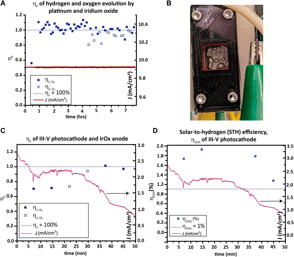
FIGURE 15. η_F and η_STH. (A) Hydrogen and oxygen evolution faradaic efficiency (η_F) of a Pt WE and IrO_x CE in 0.5 M H₂SO₄ over 7 h. Average measured η_F is 103% +/− 5% for HER and 93% +/− 6% for OER, with likely sources of loss being minor system leaks and minor crossover and recombination. (B) Hydrogen evolution from a Pt foil electrode in the test vessel during the η_F measurement in (A). (C) H₂ and O₂ η_F of a GaInP/GaAs photocathode and IrO_x anode in a two-electrode CA measurement. (D) η_STH calculated from (C).

Membrane Crossover Quantification

While proton exchange membranes such as Nafion selectively transport protons while excluding anionic species, they have some permeability to gases. The permeation of H₂ from the cathode chamber to the anode chamber through the membrane (i.e., membrane crossover) is estimated by quantifying the H₂ detected in the anode outlet with GC. This provides a lower bound to the crossover because H₂/O₂ recombination may occur when mixed in the anolyte, which may lead to underestimation of crossover. Because crossover decreases η_STH of a photocathode, anything observed should be reported along with η_STH.

Durability Characterization

Durability testing can be done simultaneously with η_STH measurement to obtain the total H₂ evolved over the device lifetime and the rate changes of H₂ evolution with time. For the development of materials that are viable for deployment in bias-free solar water-splitting devices that can compete with hydrocarbon-based hydrogen generation, it is thought that a lifetime of over 30,000 h on the sun will be required (Nandjou and Haussener, 2017). Given that today many devices do not survive for 100 h, it is clear that measuring and improving durability is important.

Definitions and Acronyms for PEC Water Splitting

This section presents the acronyms used in PEC water splitting to ensure that the literature is consistent between research groups.

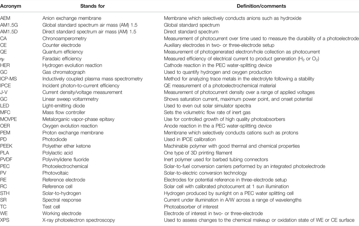
Current sign: the convention in the PEC field is for cathodic currents, with electrons flowing into the electrolyte from the photoelectrode, to be designated as negative. Anodic currents are designated as positive.

Data availability statement

The raw data supporting the conclusions of this article will be made available by the authors without undue reservation and at HydroGEN Data Hub (http://datahub.h2awsm.org/).

Author Contributions

All the authors contributed to and read the final version of the manuscript.

Conflict of Interest

The authors declare that the research was conducted in the absence of any commercial or financial relationships that could be construed as a potential conflict of interest.

The handling editor CX declared a past co-authorship with the author TD.

Publisher’s Note

All claims expressed in this article are solely those of the authors and do not necessarily represent those of their affiliated organizations or those of the publisher, the editors, and the reviewers. Any product that may be evaluated in this article, or claim that may be made by its manufacturer, is not guaranteed or endorsed by the publisher.

Acknowledgments

The authors gratefully acknowledge research support from the HydroGEN Advanced Water Splitting Materials Consortium, established as part of the Energy Materials Network under the U.S. Department of Energy, Office of Energy Efficiency and Renewable Energy, Hydrogen and Fuel Cell Technologies Office. This work was authored in part by the National Renewable Energy Laboratory, operated by Alliance for Sustainable Energy, LLC, for the U.S. Department of Energy under Contract Number DE-AC36-08GO28308 for National Renewable Energy Lab and under Contract no. DE-AC02-05CH11231 for Lawrence Berkeley National Laboratory. The views expressed in the article do not necessarily represent the views of the DOE or the U.S. Government. By accepting the article for publication, the publisher acknowledges that the U.S. Government retains a nonexclusive, paid-up, irrevocable, worldwide license to publish or reproduce the published form of this work or allow others to do so for the U.S. Government purposes. The authors thank Peter Agbo for the insightful discussions.

References

Cendula, P., Steier, L., Losio, P. A., Grätzel, M., and Schumacher, J. O. (2018). Analysis of Optical Losses in a Photoelectrochemical Cell: A Tool for Precise Absorptance Estimation. Adv. Funct. Mat. 28 (1), 1702768. doi:10.1002/adfm.201702768

CrossRef Full Text | Google Scholar

Chen, Z., Dinh, H. N., and Miller, E. (2013). Photoelectrochemical Water Splitting. Springer.

Google Scholar

Chen, Z., Jaramillo, T. F., Deutsch, T. G., Kleiman-Shwarsctein, A., Forman, A. J., Gaillard, N., et al. (2011). Accelerating Materials Development for Photoelectrochemical Hydrogen Production: Standards for Methods, Definitions, and Reporting Protocols. J. Mat. Res. 25 (1), 3–16. doi:10.1557/jmr.2010.0020

CrossRef Full Text | Google Scholar

Döscher, H., Geisz, J. F., Deutsch, T. G., and Turner, J. A. (2014). Sunlight Absorption in Water – Efficiency and Design Implications for Photoelectrochemical Devices. Energy & Environ. Sci. 7 (9), 2951–2956.

Google Scholar

Döscher, H., Young, J. L., Geisz, J. F., Turner, J. A., and Deutsch, T. G. (2016). Solar-to-hydrogen Efficiency: Shining Light on Photoelectrochemical Device Performance. Energy & Environ. Sci. 9 (1), 74–80.

CrossRef Full Text | Google Scholar

Dunbar, R. B., Barbe, A., and Fell, C. J. (2015). An Optical Imaging Method for High-Accuracy Solar Cell Area Measurement. IEEE J. Photovoltaics 5 (5), 1422–1427. doi:10.1109/jphotov.2015.2457297

CrossRef Full Text | Google Scholar

Kistler, T. A., Danilovic, N., and Agbo, P. (2019). Editors' Choice-A Monolithic Photoelectrochemical Device Evolving Hydrogen in Pure Water. J. Electrochem. Soc. 166 (13), H656–H661. doi:10.1149/2.1151913jes

CrossRef Full Text | Google Scholar

Moon, C., Seger, B., Vesborg, P. C. K., Hansen, O., and Chorkendorff, I. (2020). Wireless Photoelectrochemical Water Splitting Using Triple-Junction Solar Cell Protected by TiO2. Cell Rep. Phys. Sci. 1 (12), 100261. doi:10.1016/j.xcrp.2020.100261

CrossRef Full Text | Google Scholar

Moriarty, T., Jablonski, J., and Emery, K. (2012). Algorithm for Building a Spectrum for NREL's One-Sun Multi-Source Simulator, 001291-001295. Golden, CO, United States: National Renewable Energy Lab.

Google Scholar

Nandjou, F., and Haussener, S. (2017). Degradation in Photoelectrochemical Devices: Review with an Illustrative Case Study. J. Phys. D. Appl. Phys. 50 (12), 124002. doi:10.1088/1361-6463/aa5b11

CrossRef Full Text | Google Scholar

Osterwald, C. R. (1986). Translation of Device Performance Measurements to Reference Conditions. Sol. Cells 18 (3), 269–279. doi:10.1016/0379-6787(86)90126-2

CrossRef Full Text | Google Scholar

Steiner, M. A., and Geisz, J. F. (2012). Non-linear Luminescent Coupling in Series-Connected Multijunction Solar Cells. Appl. Phys. Lett. 100 (25), 251106. doi:10.1063/1.4729827

CrossRef Full Text | Google Scholar

Steiner, M. A., Kurtz, S. R., Geisz, J. F., Mcmahon, W. E., and Olson, J. M. (2012). Using Phase Effects to Understand Measurements of the Quantum Efficiency and Related Luminescent Coupling in a Multijunction Solar Cell. IEEE J. Photovoltaics 2 (4), 424–433. doi:10.1109/jphotov.2012.2206566

CrossRef Full Text | Google Scholar

Wang, Z., Hisatomi, T., Li, R., Sayama, K., Liu, G., Domen, K., et al. (2021). Efficiency Accreditation and Testing Protocols for Particulate Photocatalysts toward Solar Fuel Production. Joule 5 (2), 344–359. doi:10.1016/j.joule.2021.01.001

CrossRef Full Text | Google Scholar

Xu, Y., Wang, C., Huang, Y., and Fu, J. (2021). Recent Advances in Electrocatalysts for Neutral and Large-Current-Density Water Electrolysis. Nano Energy 80, 105545. doi:10.1016/j.nanoen.2020.105545

CrossRef Full Text | Google Scholar

Young, J. L., Steiner, M. A., Döscher, H., France, R. M., Turner, J. A., and Deutsch, T. G. (2017). Direct Solar-To-Hydrogen Conversion via Inverted Metamorphic Multi-Junction Semiconductor Architectures. Nat. Energy 2 (4), 17028. doi:10.1038/nenergy.2017.28

CrossRef Full Text | Google Scholar

Zeng, G., Pham, T. A., Vanka, S., Liu, G., Song, C., Cooper, J. K., et al. (2021). Development of a Photoelectrochemically Self-Improving Si/GaN Photocathode for Efficient and Durable H2 Production. Nat. Mat. 20 (8), 1130–1135. doi:10.1038/s41563-021-00965-w

CrossRef Full Text | Google Scholar

Zou, X., and Zhang, Y. (2015). Noble Metal-free Hydrogen Evolution Catalysts for Water Splitting. Chem. Soc. Rev. 44 (15), 5148–5180. doi:10.1039/c4cs00448e

CrossRef Full Text | Google Scholar