Time-Adaptive Transient Stability Assessment Based on the Gating Spatiotemporal Graph Neural Network and Gated Recurrent Unit

1 Introduction

Power system transient stability refers to the ability of each generator to maintain synchronous operation after a power system is greatly disturbed. At present, with the continuous expansion of the power system scale and the continuous growth of power consumption, accidents occur frequently when the system load reaches the limit transmission capacity. It leads the system closer to the limit of safe and stable operation. As long as the disturbance is slightly increased, the system will produce obvious voltage and frequency offsets, which will further lead to more serious transient stability problems (Liu et al., 2007). Therefore, the real-time assessment of transient stability after disturbance has attracted much attention.

Traditionally, transient stability assessment (TSA) has been modeled by solving a set of high-order differential algebraic equations (DAEs). It uses a direct method (Kang et al., 2021) based on a simplified model and a time domain simulation method (Wu and Ding, 2010) based on a trajectory model to evaluate system stability. Since 1980s, the transient energy function used by the direct method has been used to evaluate system stability (Hiskens and Hill., 1989; Owusu-Mireku and Chiang., 2018). However, in the actual large-scale AC/DC hybrid system, the direct method is based on the composition equation of the second-order simplified model of the generator, which leads to inaccurate evaluation. The time domain simulation method requires complete power grid and disturbance information, which consumes a lot of computing time.

With the innovative application of synchronous vector measurement technology and high-performance calculation methods, system variables can be sampled in the form of synchronization. In order to use the abovementioned technology for accurate and fast TSA, Song et al. (2005), Gomez et al. (2011), and Huang et al. (2019) carried out some experiments on TSA using synchronous vector measurements. It can make accurate and fast TSA for specific power systems. By extracting the relationship between the historical transient data set and the stability condition, the constraints of the system from an unstable state to a stable state can be confirmed accurately. Among them, the shallow layer neural network (Tang et al., 2019) had many applications, such as the support vector machine (SVM) method mentioned in Tian et al. (2017), which is suitable for small-scale training samples with a short evaluation time. However, there is a certain randomness in manual parameter adjustment based on experience. For different research objects, the model should have different forms and parameters to improve the accuracy of online evaluation. In addition, the poor adaptability of topology also affects the accuracy of online evaluation. In recent years, a series of deep learning methods (Tan et al., 2019; Tian et al., 2020) have been developed, which are suitable for automatically extracting data features from large samples. This method is used in TSA processes, such as the long- and short-term memory (LSTM) networks (Sun et al., 2020) and the gated recurrent unit (GRU) network (Chen and Wang., 2021) in the recurrent neural network (RNN), which rely on the timeliness of data for rapid evaluation. However, this method only considers the independent time series data of each node. The significant impact of the time-varying topology on TSA is ignored. The graph neural network (GNN) model (Scarselli et al., 2009) solves the problem of topological structure influence, such as the graph convolutional neural (GCN) network in Li et al. (2020) and the graph attention network (GAT) in Zong et al. (2021). They are embedded in power grid topology. When this characteristic information is input, the spatial correlation information between nodes is extracted to improve the evaluation accuracy. However, the method outputs the evaluation results at all times. It results in a large amount of computational data and prolongs the evaluation time. It is not beneficial for the stable recovery of the system.

The abovementioned deep learning models only consider the time-varying or topological space-varying data. They have a limitation between the time and accuracy of coordinated evaluation. At present, this model has been proven to be superior in graph data structure and time series information analysis in many fields, including traffic flow prediction (Zhao et al., 2020). However, this model has not been applied in the field of power systems. The complex traffic road structure is similar to the power grid structure. It is a complex network structure connected by points and lines. Therefore, the combined model of RNN and GNN provides a new solution for quickly extracting accurate dynamic spatial topology and time information.

Therefore, based on the two models, a gating spatiotemporal graph neural network (GSTGNN) framework with embedded topology and time series information is proposed. An adaptive method (Li et al., 2018) was adopted to improve the accuracy and speed of the assessment. Compared with the GAT model using multiple attention heads equally, the GSTGNN model is used in this study. The GSTGNN model is used to extract topological information of nodes and improve the accuracy of TSA. At the same time, the time requirement of TSA for a large-scale power network emergency control center is not more than 0.04 s (Ding, 2016). The general conventional model is to aggregate all fixed time data for TSA. Therefore, an adaptive TSA method is proposed, which uses the GRU model to aggregate less time data and get accurate evaluation results quickly. In addition, the improved weighted cross entropy loss function of the K-nearest neighbor (KNN) method (Wang and Ye, 2020) was used to improve the evaluation performance. Compared with several TSA models, the proposed model can extract the sampling information of nodes more accurately and evaluate the transient stability of AC/DC heterogeneous multisource networks.

The arrangement of this study is as follows: the second part describes the improvement of the GAT network and puts forward the GSTGNN network. The combination of GSTGNN and GRU networks is introduced in detail to form the evaluation model of this study. The third part describes the adaptive TSA process based on the model in detail, including off-line training and online evaluation. Finally, the fourth part compares the evaluation performance of the proposed method with other methods through experiments and draws a conclusion.

2 Neural Network Framework of the Gated Spatiotemporal Graph

2.1 Graph Neural Network and Attention Mechanism

The graph neural network uses the $\text{G}\left(x,A\right)$ matrix to describe the topological relationship of the power system network, where x represents the collected power grid information feature vector and A represents the adjacency matrix of the topology. The application of the graph neural network in the power system is to aggregate the information of $\text{G}\left(x,A\right)$ having a topological relationship. It can aggregate the characteristics of nodes themselves and neighbors and generate a new feature $\text{G}\left(\tilde{x},A\right)$. $\text{G}\left(\tilde{x},A\right)$, containing original information and topological information, has a higher correlation with the output results. $\tilde{x}$ represents a new feature vector with higher correlation with the evaluation results, as shown in Figure 1.

FIGURE 1

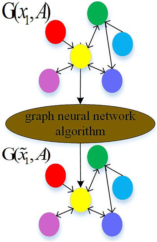
FIGURE 1. Graph of the neural network algorithm process.

The attention mechanism is introduced to weighted summation of the features of adjacent nodes. The weight is completely determined by the features of nodes, which is not affected by the dynamic topology. Each node in the model represents a monitoring node in the grid topology. The input of the attention layer of the graph is the node feature vector set x, as given below:

$x={\left(\overrightarrow{x_1},\overrightarrow{x_2},\dots ,\overrightarrow{x_N}\right)}^T, \overrightarrow{x_i}\in R^F.(1)$

Here, $\overrightarrow{x_i}$ is the eigenvector of node i, N is the number of system nodes, and F is the characteristic number of nodes.

The output of each layer is a new node feature vector set $\tilde{x}$, as given below:

$\tilde{x}={\left(\overrightarrow{\widetilde{x_1}},\overrightarrow{\widetilde{x_2}},\dots ,\overrightarrow{\widetilde{x_N}}\right)}^T,\overrightarrow{\widetilde{x_i}}\in R^F.(2)$

Here, $F^{\prime }$ is the feature number of the new node, similar to the feature extractor.

For N nodes, input node features predict output new node features. The operation of $\text{G}\left(\tilde{x},A\right)$ obtained from $\text{G}\left(x,A\right)$ first needs to calculate the attention coefficient $a_{ij}$, as given below:

$a_{ij}=softmax\left(e_{ij}\right)=\frac{\text{exp}\left(\eta \left(\beta \cos \left(W\overrightarrow{x_i},W\overrightarrow{x_j}\right)\right)\right)}{{{\displaystyle \sum }}_{k\in N_i}\text{exp}\left(\eta \left(\beta \cos \left(W\overrightarrow{x_i},W\overrightarrow{x_k}\right)\right)\right)}.(3)$

Here, the matrix W is initialized, β is the training parameter, cos is the cosine similarity, and $\eta$ is the LeakyReLU nonlinear activation function.$\widetilde{a_{ij}}$ is determined in Eq. 4 through the adjacency matrix A

$\widetilde{a_{ij}}=\{\begin{array}{l}{a}_{ij } A_{ij}=1\\ 0 A_{ij}=0\end{array}.(4)$

Different attention coefficients are generated during each training. Therefore, this study proposes a network structure using a new attention head mechanism. It sets the weight for the important attention head containing topology information, that is, 0 to 1. The model pays attention to the node information of the important attention head and improves the interpretability of the model.

For a GAT layer with k attention heads, each attention head contains a different set of parameters W and $a_{ij}$. $m_i$ represents a vector composed of k attention head weights. The working process is shown in Figure 2.

FIGURE 2

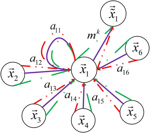
FIGURE 2. Characteristic extraction process.

Among them, node 1 has three attention heads in its neighborhood. Different arrow styles and colors represent independent attention heads. Different soft gates aggregate and control the features of each head to get more relevant feature vectors. The weight formula of attention head is shown below:

$\begin{array}{l}{m}_i=\left[m_i^{\left(1\right)},m_i^{\left(2\right)},\dots ,m_i^{\left(k\right)}\right],\\ =F{C}_{{\theta }_m}^{\alpha }\left(x_i\oplus {max}_{j\in N_i}\left(\left\{F{C}_{{\theta }_g}\left(x_j\right)\right\}\right)\oplus \frac{{{\displaystyle \sum }}_{j\in N_i}{x}_j}{\left|N_i\right|}\right),\end{array}(5)$

Here, the combined maximum pool and average pool are used to construct the network. $x_j$ is the adjacent node of node i, ${\theta }_g$ means to map the features of neighbor nodes to the vector of g dimensions as small as possible, $N_i$ is the number of neighbor nodes of node i, $F{C}_{\theta }^{\alpha }=\alpha \left(wx+b\right)$ represents the single and full connection layers, $\alpha$ is the sigmoid activation function, $\oplus$ is the linker, k is the number of attention heads, ${\theta }_m$ maps connected features to the k-dimensional space, and $m_i^{\left(k\right)}$ is the weight of the kth attention head of the ith node.

Each node i aggregates the new output features of the attention head topology information, as follows:

$\widetilde{x_i}={\parallel }_{k=1}^K{m}_i^{\left(k\right)}\sigma \left({\displaystyle \sum }_{j\mathit{ϵ}{N}_j}\widetilde{a_{ij}^k}{W}^k{x}_j\right).(6)$

Here, after $\widetilde{x_i}$ going by the GSTGNN layer, node i contains the output new features of the feature information of different spatial adjacent nodes. The attention head k satisfies inequality $k\ge 2$. σ represents the GELU activation function (Hendrycks and Gimpel., 2016).

In order to prevent overfitting of the model, the random regularization idea is introduced to control the performance on the training set, as follows:

$\begin{array}{l}\text{GELU}s\left(x\right)=x\varphi \left(x\right),\\ =0.5x\left(1+tanh\left[\sqrt{\frac{2}{\pi }}\left(x +0.044715x^3\right)\right]\right).\end{array}(7)$

Here, $\phi \left(x\right)$ uses N (0,1) normal distribution.

When x decreases, the output value will depend on the input value randomly according to the probability. It improves the generalization ability of the model.

2.2 Gated Recurrent Unit

As mentioned before, GSTGNN is introduced to extract power grid topology information to improve the evaluation accuracy. However, the evaluation time is not considered. The system studied in this study is a high-dimensional dynamic system. Not only each node has power grid topology information but also its physical quantity has time series characteristics. The GRU network has the characteristics of forgetting and selective memory. It learns and retains the timing characteristics of input data for later use. In transient assessment, the stability after fault removal can be deduced from the fault state. Therefore, the GRU layer is added to capture the historical sequence and current information of nodes and predict the future time stability. It does not need to input all time data. Thus, it can shorten the evaluation time.

In conclusion, in order to process the sequence information with a complex topological structure and time correlation, GSTGNN and GRU are combined to form a gated spatiotemporal GNN framework. At each time, the input $x_t$ and hidden state $h_{t-1}$ get new features ${\tilde{x}}_t$, ${\tilde{h}}_{t-1}$ with topology information through the GSTGNN layer, as follows:

$\begin{array}{l} {\tilde{x}}_t=\text{G}\left(x_t,A\right),\\ {\tilde{h}}_{t-1}=\text{G}\left(h_{t-1},A\right).\end{array}(8)$

Here, two gating states $z_t$ and $r_t$ are obtained by the state transmitted from the previous node $\widetilde{h_{t-1}}$ and the input of the current node $\widetilde{x_t}$; $z_t$ is the gating of control update, which decides the unit to update its active content to reduce the risk of gradient disappearance; $r_t$ is the gating of control reset, which determines the degree of combining the new input information with the previous memory state features. The expression is shown as follows:

$\begin{array}{l}{z}_t=\alpha \left(W_z\widetilde{x_t\left[i,:\right]}+b_z\right),\\ r=\alpha \left(W_r\widetilde{x_t\left[i,:\right]}+U_r\widetilde{h_{t-1}\left[i,:\right]}+b_r\right).\end{array}(9)$

Here, α is the sigmoid activation function with a range of (0,1).

Through $r_t$, the new memory will store the information related to the past in the following:

$\widehat{h_t\left[i,:\right]}=\text{tanh}\left(W_h\widetilde{x_t\left[i,:\right]}+U_h\left(r_t\odot U_h\widetilde{h_{t-1}\left[i,:\right]}\right)+b_h\right).(10)$

Here, $\odot$ means the Hadamard product and multiplies the corresponding elements in the matrix to identify retained and forgotten previous information. $\widehat{h_t\left[i,:\right]}$ remembers the state of previous time by resetting.

The memory state of current time step $h_t\left[i,:\right]$ needs $z_t$ to forget and select memory at the same time as follows:

$h_t\left[i,:\right]=\left(1-z_t\right)\odot \widetilde{h_{t-1}\left[i,:\right]}+z_t\odot \widehat{h_t\left[i,:\right]}.(11)$

Here, $\left(1-z_t\right)\odot \widetilde{h_{t-1}\left[i,:\right]}$ means selective “forgetting” of the original hidden state and removing unimportant information. $z_t\odot \widehat{h_t\left[i,:\right]}$ selects some information in $\widehat{h_t\left[i,:\right]}$, which means forgetting the state information of the past moment and adding some state information input by the current node. In order to improve the generalization ability and evaluation accuracy of the model, topology information is included in the transmission of the abovementioned state information.

Finally, new features aggregated are input into the softmax separator for classification. The output prediction value $\tilde{y}$ at the last time is obtained in Eq. 12. The value range is (0,1)

$\tilde{y}=softmax\left(W_o{h}_{last}\left[i,:\right]+b_o\right).(12)$

Here, $W_o$ and $b_o$ are the parameters learned by gradient back propagation.

3 Adaptive Transient Stability Assessment

3.1 Principle

In order to start the emergency control immediately after the fault is removed, TSA needs to be performed quickly and accurately. In Sun et al. (2020) and Tian et al. (2020), most of the existing TSA methods use a fixed length observation window; that is, the evaluation time is constant. However, this static evaluation time may not be able to cope with fast transient instability. The system models with different fault degrees need different observation window lengths. After the fault is removed, the dynamic data of the system are observed in the dynamic time window. The stability of the system is evaluated in the future time window, and the observation time window is gradually adjusted. As long as the evaluation system loses stability in the future, the emergency control will be started immediately.

3.2 Off-Line Training

3.2.1 Generate Data Set

The purpose of the evaluation model is to obtain the evaluation results from the sampling data. The input data need to fully reflect the dynamic behavior of the system. In this study, the transient stability of the power system after fault removal is studied. Rajapakse et al. (2009) proposed to use PMU to sample the generator voltage amplitude after fault as input. Due to the inertia of the rotor, it takes a long time to display the change of generator rotor speed and angle after fault. In contrast, the generator voltage amplitude reflects the fault faster than the rotor angle variable. It has been verified that the voltage amplitude can accurately evaluate the transient stability of the system. Gomez et al. (2011) further proved that the use of voltage amplitude has a higher evaluation accuracy than mechanical variables (rotor angle and angular velocity). Therefore, this study selects voltage amplitude as the input variable. In addition, other node dynamic variables are selected to form the input data together with the voltage amplitude to improve the evaluation accuracy. Li et al. (2021) selected the initial characteristics reflecting the system dynamics to construct the input characteristics of TSA. The input characteristics include voltage amplitude, phase angle, injected active power, and injected reactive power of each node on all buses.

Analog measurements are used by 50 Hz sampling. In order to better simulate the system response after various faults are removed, different contingencies are simulated to generate the whole data set. Input x is expressed in the form of time as follows:

$x={\left(x_1,x_2,\dots ,x_T\right)}^T={\left(\begin{array}{cc}{\left(\begin{array}{ccc}{u}_{\mathrm{1,1}}& \dots & u_{T,1}\\ \dots & u_{t,n}& \dots \\ u_{1,N+1}& \dots & u_{T,N+1}\end{array}\right)}^T,& {\left(\begin{array}{ccc}{\delta }_{\mathrm{1,1}}& \dots & {\delta }_{T,1}\\ \dots & {\delta }_{t,n}& \dots \\ {\delta }_{1,N+1}& \dots & {\delta }_{T,N+1}\end{array}\right)}^T,\\ {\left(\begin{array}{ccc}{p}_{\mathrm{1,1}}& \dots & p_{T,1}\\ \dots & p_{t,n}& \dots \\ p_{1,N+1}& \dots & p_{T,N+1}\end{array}\right)}^T,& {\left(\begin{array}{ccc}{q}_{\mathrm{1,1}}& \dots & q_{T,1}\\ \dots & q_{t,n}& \dots \\ q_{1,N+1}& \dots & q_{T,N+1}\end{array}\right)}^T,\end{array}\right)}^T,(13)$

Here, $u_{t,n}$, ${\delta }_{t,n}$, and $p_{t,n}$ and $q_{t,n}$ are the node voltage amplitude, phase angle, and active and reactive power, respectively; T is the observation time window, which affects the accuracy and complexity of GRU evaluation; and N is the number of nodes, which is determined by the grid topology.

The transient stability index (TSI) of the power angle after fault removal is used to judge the sample stability. The expression is shown as follows:

$y_i=\{\begin{array}{c}1 \left(Stable\right) t\succ 0\\ 0 \left(Unstable\right) t\le 0\end{array} i=\mathrm{1,2},\mathrm{...},T.(14)$

Here, t satisfies the formula $t=\frac{360-{\delta }_{max}}{360+{\delta }_{max}}$. ${\delta }_{max}$ is the maximum power angle difference of any two synchronous generators at the end of the simulation, and $y_i$ is the label of the real category (Xie et al., 2021). A complete data set is established.

3.2.2 Improved Weighted Cross Entropy Loss Function

In a really large power grid, because the number of stable samples is much larger than the number of unstable samples, that is, “imbalance”, some important unstable situations may be misjudged as stable. In practical applications, more attention is paid to the accurate evaluation of unstable samples. Conventional methods dealing with data imbalance only consider the imbalance of the number of two types of samples, while ignoring the spatial distribution information of the number of two types of samples (Chen et al., 2017).

The KNN method (Wang and Ye, 2020) can obtain the spatial distribution information of each sample so as to solve the problem of data imbalance. First, the distance between each sample and the nearest sample of the opposite category is calculated. It is the reference position of the sample, which is used to divide the region. Then, the number of unstable and stable data of a series of location regions is obtained, which is the spatial distribution of the sample.

The study sets the total space to have a areas. The formula is shown as follows:

$w_{A_i}=\frac{F_{B_i}}{F_{A_i}+F_{B_i}}{w}_{B_i}=\frac{F_{A_i}}{F_{A_i}+F_{B_i}},(15)$

Here, $F_{A_i}$ and $F_{B_i}$ are the number of unstable and stable samples in ith region. $w_{A_i}$ (i = 1,2, …, a) and $w_{B_i}$ (i = 1,2, …, a) are the weights of samples in the ith region.

In this study, an improved weighted cross entropy loss function is used to increase the cost of misjudgment, as follows:

$L=-\frac{1}{N}{\displaystyle \sum }_{j=1}^N\left(w_{A_i}{y}_{j}log\left({\tilde{y}}_j\right)+w_{B_i}\left(1-y_j\right)log\left(1-{\tilde{y}}_j\right)\right).(16)$

Here, N is the number of single training samples, $y_j$ is the label of real class, and ${\tilde{y}}_j$ is the probability of evaluation class.

The purpose of off-line training is to get the optimal w and b by using the Adam optimizer to train the model under the condition of minimum loss function L. The abovementioned methods are used to reduce the impact of unbalanced data.

3.3 Online Evaluation

The stability threshold is used to evaluate the evaluation results. Because the GRU layer is used in this study, ${\tilde{\text{y}}}_i$ only focuses on the stability index generated at time T. When i = 1, 2,..., T − 1 is ignored, the rule is shown as follows:

$Stability=\{\begin{array}{l}Stable 1\ge {\tilde{y}}_i>\delta \\ Unstable {\tilde{y}}_i<1-\delta i=\mathrm{1,2},\mathrm{...},T\\ Unknow Others\end{array}.(17)$

Here, $\delta \in \left(0.5,1\right)$ is the stability threshold.

It is necessary to search and set the appropriate threshold $\delta$ to balance the accuracy of TSA with the average evaluation time. An adaptive TSA process is proposed in Figure 3.

FIGURE 3

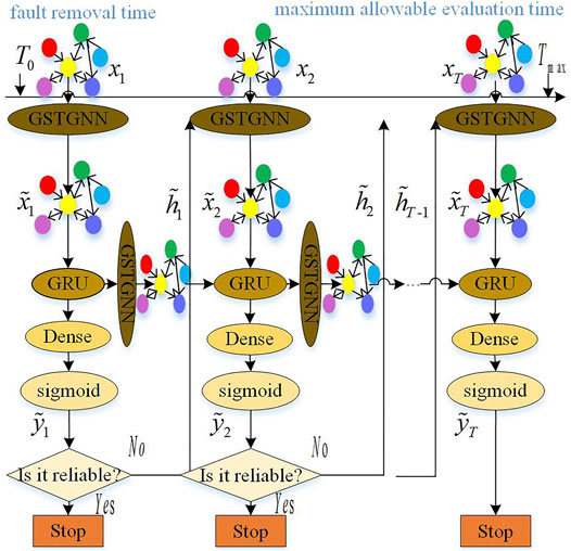
FIGURE 3. Adaptive TSA process.

In this study, $x_i$ is input to the model according to the observation time window after fault removal. The evaluation results are predicted moment by moment. When it is within the judgment range, the results are directly output. Otherwise, the hidden state $h_i$ at this time and the next time $x_{i+1}$ are input to the next neuron for TSA. If the evaluation time exceeds the observation time window, the sliding time window method is adopted until the reliable evaluation result. $\widetilde{y_i}$ is obtained, or the maximum allowable evaluation time $\left(T_{max}\right)$ is reached. If $T_{max}$ has not been determined, it is regarded as unstable. In this process, $h_i$ and $x_{i+1}$ are needed to go through the GSTGNN layer to get $h_i$ and $x_{i+1}$ with topological relationship and inputed to the next evaluation time. It is found that $T_{max}$ is generally set to 10 cycles.

3.4 TSA Performance Comparison

With the continuous development of machine learning, for the classification problem, the index based on the confusion matrix in Table 1 can better evaluate the applicability of the classification model than only using the accuracy.

TABLE 1

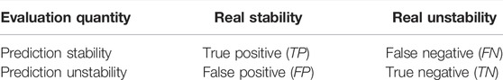
TABLE 1. Confusion matrix for TSA.

In the power system transient stability analysis, researchers pay more attention to whether the instability is classified correctly. As a result, the following evaluation indexes are mainly based on whether the instability can be correctly judged. In Table 1, TP is the number of stable samples correctly predicted, FP is the number of unstable samples incorrectly predicted, FN is the number of mispredicted stable samples, and TN is the number of unstable samples correctly predicted. In the confusion matrix, the more the number of TP and TN is, the better the number of FP and FN is. However, there are a large number of sample data. It is difficult to measure the model only by the number. Therefore, in order to comprehensively evaluate the TSA performance, four indexes are obtained as follows to calculate the accuracy (ACC), miscalculation rate (recall), precision, and comprehensive evaluation index $\left(F_1\right)$ of the model instability.

ACC is the proportion of the number of correct assessments to the total number of assessments, defined as follows:

$ACC=\frac{TP+TN}{TP+TN+FP+FN}\times 100\% .(18)$

Once an unstable situation is misjudged as a stable situation, it may lead to a large area power outage of the system. Thus, the unstability recall is used to express the misjudgment rate. The closer the recall is to 1, the lower the possibility of misjudgment of the unstability situation. The formula of recall is shown as follows:

$recall=\frac{TN}{TN+FP}\times 100\% .(19)$

Unstability precision is the proportion of correctly predicted unstable samples, defined as follows:

$precision=\frac{TN}{TN+FN}.(20)$

The higher the precision is, the more accurate it is to predict the unstable situation. However, recall and precision are inversely proportional and cannot reach a high ratio at the same time. Therefore, $F_1$, the weighted harmonic average of precision and recall, is introduced in Eq. 21. The two performance indicators are comprehensively considered. $F_1$ is distributed between [0,1]. The closer it is to 1, the stronger the feature extraction ability of the model and the better the evaluation performance

$F_1=\frac{2\times precision\times recall}{precision\times recall}.(21)$

The accuracy mainly includes ACC and $F_1$. Although the deep learning algorithm studied in this study can reach 1 (or 100%) in theory, it will lead to overfitting of the model. The data model does not have enough prediction ability. Therefore, this study introduces the idea of stochastic regularization, which is as close as 100% when the prediction requirements are met.

Besides the accuracy, the average response time (ART) in Eq. 22 is also an important index to evaluate the performance of TSA

$ART={\displaystyle \sum }_{i=1}^{T_{max}}\left[T_i\times C\left(T_i\right)\right]/{\displaystyle \sum }_{i=1}^{T_{max}}C\left(T_i\right).(22)$

Here, $T_{max}$ is the maximum allowable evaluation time (10 cycles). $C\left(T_i\right)$ is the total number of classified instances in the current evaluation cycle. ART refers to the average TSA time after fault removal.

3.5 Total Evaluation Process

The total TSA process is shown in Figure 4:

FIGURE 4

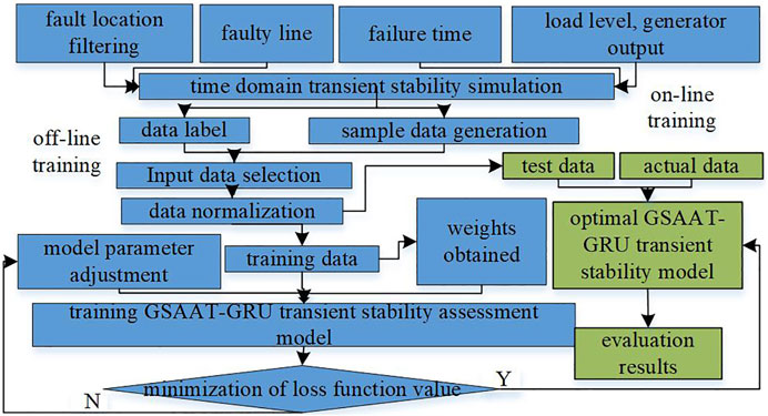
FIGURE 4. General evaluation flow chart.

1) Off-line training: In this study, the three-phase permanent short-circuit fault is set under different fault points of different lines. It can realize the diversity of sample data. The time domain simulation method generates data, including voltage amplitude, phase angle, injected active power, injected reactive power, and the maximum power angle difference ${\delta }_{max}$ at the end of the simulation. ${\delta }_{max}$ obtains the stability index t; when t > 0, it indicates the system transient stability, and the label is “1"; on the contrary, the system is unstable and the label is “0". This study selects the dynamic data of each node on the bus as the input data to determine the system stability in order to be limited to a certain range to reduce the difference of the data. The training data and test data are generally normalized. The weights under instability and stability are obtained from the training data so as to form a weighted cross entropy loss function. The model parameters are continuously adjusted. The Adam method is used to minimize the loss function until the optimal evaluation model is obtained.

2) Online evaluation: Test data and actual data are added, and performance is evaluated by using the best trained model.

4 Numerical Example

4.1 Generation of Sample Data Sets

This study uses a representative New England 10-machine 39-node power system in Figure 5 to evaluate the performance of the method. The reference frequency is 50 Hz. The time domain simulation data of PSA-BPA software is used, similar to the data generated by PMU in real time. Python is used to program.

FIGURE 5

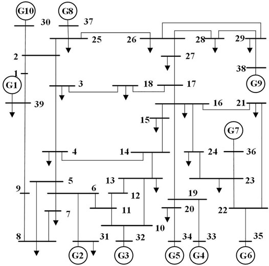
FIGURE 5. New England 10-machine 39-bus power system.

The sampling step is set as 0.02 s. Various faults are simulated in various scenarios to obtain complete data sets. A total of 11 load levels of 75–125% (step size 5%) are set. Generator output is changed accordingly to ensure power flow convergence. The Three-phase permanent short-circuit fault is set for the fault type. Fault points are set for 0, 25, 50, 75, and 100% of lines. The fault clearing time is set for 0.2 s. The simulation time is 5 s. Fault samples are selected considering the whole wiring system and N-1 accident. The fault samples are 8855. A total of 6000 training set samples are randomly selected, and test set samples are selected according to 4:1, including 5211 stable samples and 2289 unstable samples.

In order to train the evaluation model with the best performance, these control parameters are defined later. In terms of the model structure, this study sets up two GSTGNN input layers to avoid excessive smoothing caused by too many layers. One GSTGNN middle layer and four attention heads are set to extract and aggregate the features with the topological structure of the power grid. The GRU layer is set to two layers, with 128 batch sizes in each layer, which further improves the evaluation speed. The last layer is the dense layer, which uses the nonlinear activation function to fit the nonlinear problem to improve the evaluation accuracy. In terms of training parameters, the dropout is set to 0.05. The learning rate is set to 0.001. The training iterations are set to 300. The aforementioned settings can improve the performance of the evaluation model.

In the test, each evaluation cycle of the adaptive TSA method based on the sampling step is 0.02 s. The maximum evaluation time is set to 0.2 s ($T_{\max }$ = 10). The observation window T and δ are set to 8 and 0.62, respectively. The specific setting experiment is described later.

4.2 Handling Unbalanced Data

In this study, the idea of KNN is introduced to calculate the weight of each sample. The weight is added to the training parameters in the loss function to obtain the best model. A total of 6000 samples with or without imbalance are taken as the training data. The number of iterations is 300. When T = 8, δ = 62; the training process is shown in Figure 6.

FIGURE 6

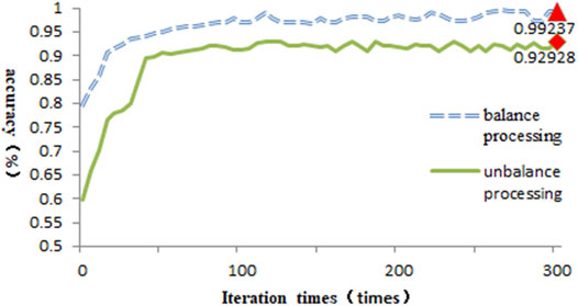
FIGURE 6. Relationship between iteration times and accuracy.

After the fault occurs, with the increase of iteration times, the accuracy (ACC) increases rapidly until it reaches 50 times. The accuracy tends to increase gently. Finally, the evaluation accuracy of balanced processing can reach 99.237%. Therefore, data quality has an important influence on the training high-performance model.

For the same set of data, the performance of this method is improved compared with other deep learning models, as shown in Table 2.

TABLE 2

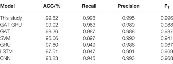
TABLE 2. Model performance comparison.

According to Table 2, the recall of SVM which belongs to the shallow model is less than 0.9, so it cannot extract features accurately and is prone to misjudgment. GAT, LSTM, and GRU models all have higher ACC. However, when the scale of system topology expands, the $F_1$ value of the GAT model is higher than that of LSTM and GRU models. It indicates the importance of topological relationship between nodes for TSA. Because the CNN model does not take into account the topological structure and time series information of the power grid, ACC is relatively low. Compared with the previous model, the ACC of the framework established in this study is closer to 100%, and the $F_1$ value is relatively close to 1. It still has strong generalization performance for high-dimensional data. The framework is relatively more stable. Its performance is better than that of GAT-GRU, GAT, SVM, GRU, LSTM, and CNN models. This indicates that this framework can better mine the essential characteristics of data. Its training parameter sharing overcomes the complex problems of the traditional adaptive evaluation system.

4.3 Average Evaluation Time and Training Time

The following table shows the comparison of art and training time in Table 3.

TABLE 3

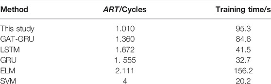
TABLE 3. Average evaluation time versus training time.

The ART of the GRU model and LSTM model are basically the same (Yu et al., 2018). Because the parameters of the GRU model are less than those of the LSTM model, the training time is relatively short (Chen and Wang. 2021). The extreme learning machine (ELM) network (Zhang et al., 2015) needs to train 10 classifiers whose parameters are not shared. A large number of parameters lead to the longest training time. A simple SVM network structure cannot effectively extract features, resulting in the longest ART. This method extracts the topological relationship and time series information of important attention heads. This method feature extraction ability is higher than that of the GAT-GRU model, which only extracts the topological relationship of attention heads on average. Thus, the output results are easier to reach the stability threshold, and the TSA evaluation speed is faster. In the case of ensuring a high accuracy, the ART of this study is 1.01 cycles, which meets the requirements of emergency control. At the same time, although the model layers of this study and GAT-GRU are more and the offline training time is longer than those of the GRU model and LSTM model, it does not affect the effect of online evaluation. This model is still practical.

4.4 Observation Time Window T and Stability Threshold δ Test

In this study, these two parameters T and δ affect the evaluation performance. The following figures in Figure 7 and Figure 8 are the histograms of ACC and ART, respectively.

FIGURE 7

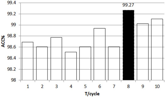
FIGURE 7. T on the relationship of accuracy.

FIGURE 8

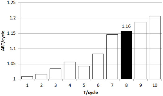
FIGURE 8. T on the relationship of ART.

When T = 8, it means that after the fault is cleared, the input data of the first eight cycles are used for training and continuous time series data are used for testing. The maximum accuracy is about 99.27%, which shows that the input data affect the system performance. With the increase of T, the overall trend of ACC increases (there is a small fluctuation), and the TSA time is longer. The shorter T may damage the integrity of the input data, reducing the accuracy. Therefore, in the case of T as small as possible to ensure a high accuracy, T = 8 is the best choice.

When T = 8, δ for the histogram of ACC and ART is obtained in Figure 9 and Figure 10.

FIGURE 9

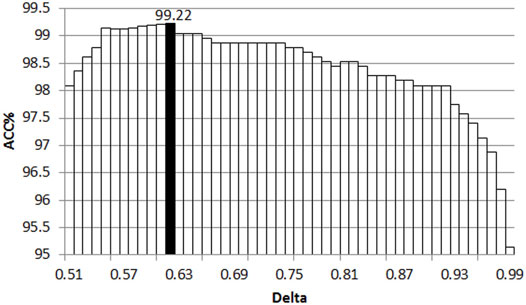
FIGURE 9. δ on the relationship of accuracy.

FIGURE 10

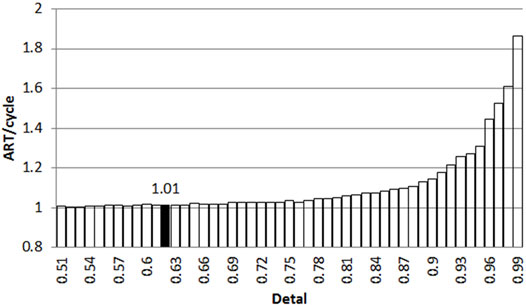
FIGURE 10. δ on the relationship of ART.

As with the observation time window, the size of δ also affects ACC and ART. The smaller δ may lead to earlier evaluation. However, the accuracy rate may be reduced, while the larger δ produces more accurate results at the expense of evaluation speed. As can be seen from Figures 9, 10, the increase of δ leads to the reduction of ACC and the increase of ART. Small ART and high ACC are the expected results, so the stability threshold of 0.62 is the best.

To sum up, T is set to 8. δ is set to 0.62 to get the fastest evaluation time without reducing the accuracy.

4.5 Test of Topology Change

After the fault is removed, the adaptability of the model to topology changes is tested. Four changes are listed in the following table, and 1500 test sets are selected for the performance test in Table 4.

TABLE 4

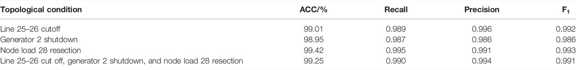
TABLE 4. Results of TSA under topological structure change.

It is found from Table 4 that the accuracy of TSA caused by generator shutdown is the lowest, but it is still more than 99% when the load is cut off. In general, the TSA accuracy of this model is still about 99% in the case of topology changes. The results show that the features selected in this study are enough to reveal the system state of the power grid in the case of large disturbance. The selected model can fully mine the transient variation law and extract data features. The model with strong robustness is suitable for complex topology.

4.6 Data Visualization

t-Distributed stochastic neighbor embedding (t-SNE) for the extracted feature data is conducive to visually verify the effectiveness of the algorithm. The following is the feature map of different layers of the GSTGNN framework in Figure 11, Figure 12, and Figure 13.

FIGURE 11

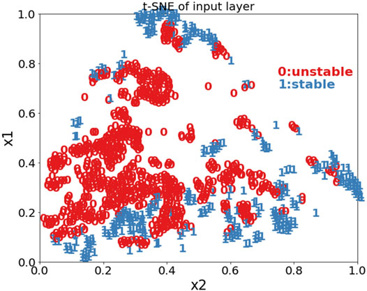
FIGURE 11. Input layer.

FIGURE 12

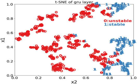
FIGURE 12. GRU layer.

FIGURE 13

FIGURE 13. Dense layer.

t-SNE is used to establish linear projection. The mapping relationship between approximate high-dimensional data space and low-dimensional embedded space is obtained. The high-dimensional input data are mapped to the two-dimensional space. The stability classification is explained intuitively. Figure 11, Figure 12, and Figure 13 show the characteristic diagrams of the input layer, GRU layer, and full dense layer of the model. With the deepening of the layer, the boundary between the two categories is more and more obvious, and the spatial overlapping data are less and less. It shows that the GSTGNN framework plays an important role in deep structure level extraction. Finally, it achieves an obvious classification effect.

5 Conclusion

In this study, a power system adaptive TSA method based on GSTGNN is proposed. It learns spatial and temporal correlation of data to balance assessment accuracy and assessment time. The New England 10-machine 39-bus system is used for verification, compared with a variety of verification algorithms to indicate the following:

1) This study introduces the graph attention depth learning network and considers the topological relationship between nodes. It also proposes a new attention head mechanism, which considers the feature correlation of adjacent nodes from important attention heads. In the process of aggregation, the new characteristics of nodes will change according to the changes of topology and attention coefficient. Therefore, the use of GNN can improve the evaluation accuracy and is more suitable for the changing and complex power grid structure.

2) This study uses adaptive TSA and GRU layers to capture the characteristic quantity of input data every moment. As long as the output data reach the threshold, the result is directly output. Thus, we can achieve rapid and accurate assessment with less data.

3) In addition to TSA performance and the response time test, two basic parameters are introduced for the preliminary sensitivity test: stability threshold and training observation window length. The simulation results show that the parameter configuration has good performance to promote the improvement of evaluation performance.

In conclusion, the composite framework is specially used to model sequence data with complex topology and time correlation. It reduces the training time and response time without sacrificing the evaluation accuracy. It is suitable for a more complex large-scale power grid research. However, the actual noise interference will affect the accuracy of the evaluation results, which needs to be considered in the future.

Data Availability Statement

The original contributions presented in the study are included in the article/Supplementary Materials, further inquiries can be directed to the corresponding author.

Author Contributions

Conceptualization, JL; methodology, CY and LC; investigation, CY; software, CY and LC; resources, JL; data curation, LC; writing—original draft preparation, CY and LC; writing—review and editing, CY; visualization, LC; project administration, JL. All authors have read and agreed to the published version of the manuscript.

Funding

This study is supported by the National Natural Science Foundation of China (51807114).

Conflict of Interest

The authors declare that the research was conducted in the absence of any commercial or financial relationships that could be construed as a potential conflict of interest.

Publisher’s Note

All claims expressed in this article are solely those of the authors and do not necessarily represent those of their affiliated organizations or those of the publisher, the editors, and the reviewers. Any product that may be evaluated in this article or claim that may be made by its manufacturer is not guaranteed or endorsed by the publisher.

References

Chen, Q., and Wang, H. (2021). Time-adaptive Transient Stability Assessment Based on Gated Recurrent Unit. Int. J. Electr. Power Energ. Syst. 133 (133), 107156. doi:10.1016/j.ijepes.2021.107156

CrossRef Full Text | Google Scholar

Chen, Y., Wang, Y., Kirschen, D., and Zhang, B. (2018). Model-Free Renewable Scenario Generation Using Generative Adversarial Networks. IEEE Trans. Power Syst. 33 (99), 3265–3275. doi:10.1109/TPWRS.2018.2794541

CrossRef Full Text | Google Scholar

Ding, W. (2016). Research on Fast Algorithm of Power System Transient Stability. Zhejiang, China: Zhejiang University.

Google Scholar

Gomez, F. R., Rajapakse, A. D., Annakkage, U. D., and Fernando, I. T. (2011). Support Vector Machine-Based Algorithm for Post-fault Transient Stability Status Prediction Using Synchronized Measurements. IEEE Trans. Power Syst. A Publ. Power Eng. Soc. 26 (03), 1474–1483. doi:10.1109/pes.2011.6038936

CrossRef Full Text | Google Scholar

Hendrycks, D., and Gimpel, K. (2016). Gaussian Error Linear Unit (GELUs). arXiv:1606.08415.

Google Scholar

Hiskens, I. A., and Hill, D. J. (1989). Energy Functions, Transient Stability and Voltage Behaviour in Power Systems with Nonlinear Loads. IEEE Trans. Power Syst. 4 (4), 1525–1533. doi:10.19783/j.cnki.pspc.200384

CrossRef Full Text | Google Scholar

Huang, D., Chen, S. Y., and Zhang, Y. C. (2019). Online Assessment for Transient Stability Based on Response Time Series of Wide-Area Measurement System. Power Syst. Techn. 43 (03), 286–295. doi:10.13335/j.1000-3673.pst.2018.0960

CrossRef Full Text | Google Scholar

Kang, Z. R., Zhang, Q., Chen, M. Q., and Gan, D. Q. (2021). Research on Network Voltage Analysis Algorithm Suitable for Power System Transient Stability Analysis. Power Syst. Prot. Control. 49 (03), 32–38. doi:10.19783/j.cnki.pspc.200384

CrossRef Full Text | Google Scholar

Li, J., Pan, F. L., Mei, Q. J., Xie, P. Y., Pen, Y. H., Jiang, X. F., et al. (2018). A Time-Aadaptive Method for On-Line Transient Stability Assessment of Power Systems. China: The People's Republic of China. State Intellectual Property Office. Patent CN 107993012A.

Google Scholar

Li, M., Lei, M., Zhou, T., Li, Y. L., Xiao, Y., and Yan, B. J. (2021). Transient Stability Assessment Method for Power System Based on Deep Forest. Electr. Meas. Instrumentation 58 (02), 53–58. doi:10.19753/j.issn1001-1390.2021.02.009

CrossRef Full Text | Google Scholar

Li, W., Zhang, Z., Luo, Z., Xiao, Z., Wang, C., and Li, J. (2020). “Extraction of Power Lines and Pylons from LiDAR Point Clouds Using a GCN-Based Method,” in IGARSS 2020 - 2020 IEEE International Geoscience and Remote Sensing Symposium. Waikoloa, HI, USA: IEEE (Institute of Electrical and Electronics Engineers), 2767–2770. doi:10.1109/IGARSS39084.2020.9323218

CrossRef Full Text | Google Scholar

Liu, J. Q., Tao, J. Q., Xu, X. W., and Zhang, H. P. (2007). A Survey on Research of Load Model for Stability Analysis in Foreign Countries. Power Syst. Techn. 31 (04), 11–15. doi:10.1002/jrs.1570

CrossRef Full Text | Google Scholar

Owusu-Mireku, R., and Chiang, H.-D. (2018). “A Direct Method for the Transient Stability Analysis of Transmission Switching Events,” in IEEE Power & Energy Society General Meeting. (Portland, OR, United States: IEEE (Institute of Electrical and Electronics Engineers)), 1–5. doi:10.1109/PESGM.2018.8586242

CrossRef Full Text | Google Scholar

Rajapakse, A. D., Gomez, F., Nanayakkara, O. M. K. K., Crossley, P. A., and Terzija, V. V. (2009). “Rotor Angle Stability Prediction Using Post-disturbance Voltage Trajectory Patterns,” in IEEE Power & Energy Society General Meeting IEEE, 1–6. doi:10.1109/PES.2009.5275270

CrossRef Full Text | Google Scholar

Scarselli, F., Gori, M., Tsoi, A. C., Hagenbuchner, M., and Monfardini, G. (2009). The Graph Neural Network Model. IEEE Trans. Neural Netw. 20 (1), 61–80. doi:10.1109/TNN.2008.2005605

PubMed Abstract | CrossRef Full Text | Google Scholar

Song, F. F., Bi, T. S., and Yang, Q. X. (2005). “Study on Wide Area Measurement System Based Transient Stability Control for Power System,” in International Power Engineering Conference. (Singapore: IEEE (Institute of Electrical and Electronics Engineers)), 757–760. doi:10.1109/IPEC.2005.207008

CrossRef Full Text | Google Scholar

Sun, L. X., Bai, J. T., Zhou, Z. Y., and Zhao, C. Y. (2020). Transient Stability Assessment of Power System Based on Bi-directional Long-Short-Term Memory Network. Automation Electric Power Syst. 44 (13), 64–72. doi:10.7500/AEPS20191225003

CrossRef Full Text | Google Scholar

Tan, B., Yang, J., Zhou, T., Xiao, Y., and Zhou, Q. (2019). “A Novel Temporal Feature Selection for Time-Adaptive Transient Stability Assessment,” in IEEE PES Innovative Smart Grid Technologies Europe (ISGT-Europe). (Bucharest, Romania: IEEE (Institute of Electrical and Electronics Engineers)), 1–5. doi:10.1109/ISGTEurope.2019.8905487

CrossRef Full Text | Google Scholar

Tang, Y., Cui, H., Li, F., and Wang, Q. (2019). Review on Artificial Intelligence in Power System Transient Stability Analysis. Chin. J. Electr. Eng. 39 (01), 2–13. doi:10.13334/j.0258-8013.pcsee.180706

CrossRef Full Text | Google Scholar

Tian, F., Zhou, X. X., Shi, D. Y., Chen, Y., Huang, Y. H., and Yu, Z. H. (2020). A Preventive Control Method of Power System Transient Stability Based on a Convolutional Neural Network. Power Syst. Prot. Control. 48 (18), 1–8. doi:10.19783/j.cnki.pspc.191310

CrossRef Full Text | Google Scholar

Tian, F., Zhou, X. X., and Yu, Z. H. (2017). Power System Transient Stability Assessment Based on Comprehensive SVM Classification Model and Key Sample Set. Power Syst. Prot. Control. 45 (22), 1–8. doi:10.7667/PSPC161864

CrossRef Full Text | Google Scholar

Wang, H., and Ye, W. (2020). Transient Stability Evaluation Model Based on SSDAE with Imbalanced Correction. IET Generation, Transm. Distribution 14 (11), 2209–2216. doi:10.1049/iet-gtd.2019.1388

CrossRef Full Text | Google Scholar

Wu, H. B., and Ding, M. (2010). Newton Method with Variable Step Size for Power System Transient Stability Simulation. Chin. J. Electr. Eng. 30 (7), 36–41. doi:10.13334/j.0258-8013.pcsee.2010.07.006

CrossRef Full Text | Google Scholar

Xie, P. Y., Yuan, W., Liu, Y. G., Pan, F. L., Ye, W. H., and Yang, J. (2021). Transient Stability Assessment Method in Power System Based on Active Learning. Electr. Meas. Instrumentation. 58 (05), 86–91. doi:10.19753/j.issn1001-1390.2021.05.012

CrossRef Full Text | Google Scholar

Yu, J., Hill, D. J., Lam, A. Y. S., Gu, J., and Li, V. O. K. (2018). Intelligent Time-Adaptive Transient Stability Assessment System. IEEE Trans. Power Syst. 33 (01), 1049–1058. doi:10.1109/tpwrs.2017.2707501

CrossRef Full Text | Google Scholar

Zhang, R., Xu, Y., Dong, Z. Y., and Wong, K. P. (2015). Post‐disturbance Transient Stability Assessment of Power Systems by a Self‐adaptive Intelligent System. IET Generation, Transm. Distribution 9 (3), 296–305. doi:10.1049/iet-gtd.2014.0264

CrossRef Full Text | Google Scholar

Zhao, L., Song, Y., Zhang, C., Liu, Y., Wang, P., Lin, T., et al. (2020). T-GCN: A Temporal Graph Convolutional Network for Traffic Prediction. IEEE Trans. Intell. Transport. Syst. 21 (9), 3848–3858. doi:10.1109/tits.2019.2935152

CrossRef Full Text | Google Scholar

Zong, Z., Guan, L., Su, Y. S., Yao, H. C., Huang, J. Y., and Guo, M. X. (2021). Power System Transient Stability Assessment Based on Graph Attention Deep Network. Power Syst. Techn. 45 (06), 2122–2130. doi:10.13335/j.1000-3673.pst.2020.0897

CrossRef Full Text | Google Scholar