Analysis of Transient Characteristics of Submersible Tubular Pump During Runaway Transition

Introduction

The submersible tubular pump device is an electromechanical integrated pump device that combines the pump and the submersible motor closely. Compared with the pump device using the conventional motor, it has the advantages of compact structure and convenient installation and is widely used in low-lift pumping stations such as inter-basin water transfer, agricultural irrigation, and urban drainage (Yang, 2013). With the development of submersible motor, the impeller diameter is also increasing, which puts forward new requirements for its safe and stable operation. It is generally believed that the hydraulic causes of vibration, noise, and rupture of flow passage components of the unit mainly include water excitation, blade cavitation, inlet swirl, and rotating stall. In the event of power failure, the change of working parameters of the pump device usually follows this series of complex physical flow, which will cause great damage to the pumping station unit (Chang, 2005; Xu, 2008).

At present, the research on the transient characteristics of hydraulic machinery units generally adopts the external characteristics based on the single element theory (Suter, 1966; Yang and Chen, 2003; Dorfler, 2010) or the internal characteristics (Liu and Chang, 2008; Guo et al., 2015; Zeng et al., 2015) based on one-dimensional theory to predict the changes of pressure, speed, torque, and other parameters in the transient process, but it is difficult to capture the transient characteristics of the internal flow field of the pump device. A test is the most direct method to study the transient characteristics of submersible tubular pump. However, due to the limitations of cost, environment, and technical level of operators, it is not easy to complete. With the development of computational fluid dynamics (CFD) technology, the CFD method has become a trend to study the three-dimensional transient characteristics in the transition process of hydraulic machinery. In recent years, many scholars have used the method of CFD to study the transition process of hydraulic machinery and have also achieved good results. Avdyushenko et al. (2013) proposed a three-dimensional unsteady turbulent flow calculation method for transient process simulation of hydraulic turbines. The three-dimensional numerical simulation of Reynolds-averaged Navier–Stokes equations was combined with the one-dimensional equation of elastic hydraulic shock propagation. The numerical results are in good agreement with the experimental results. Zhou and Liu (2015) used the VOF model to simulate the startup process of vertical axial flow pump and studied the change process of air sac in a siphon outlet pipe during the startup process. Li et al. (2015) carried out the unsteady numerical simulation of the transient flow in the two stages of pump startup and valve opening in a double suction centrifugal pump closed system based on the SAS-SST (scale adaptive simulation-shear stress transport) turbulence model. Li (2012) studied the influence of three different startup accelerations on the startup process of the oblique flow pump and obtained the variation laws of the instantaneous head and flow rate under different accelerations. Li et al. (2010) studied the startup process of centrifugal pump in detail. The vortex dynamics method was used to diagnose the transient flow field distribution during the startup process. The peak value of BVF (boundary vortex flux) and the BVF region with negative contribution were obtained, which provided reference for blade design. Zhang et al. (2014a) used a one-dimensional and three-dimensional coupling method to simulate the load rejection process of Francis turbine.

There are also many research studies on the calculation of hydraulic machinery power failure process. On the basis of solving the torque balance, Kan et al. (2020) and Kan et al. (2021) used the VOF (volume of fluid) model to establish the numerical calculation method of the power-off process of the S-shaped axially extended tubular pump device. The research shows that the CFD calculation results with the VOF model are closer to the experimental results. During the power-off process, the internal flow pattern of the pump device is complex, and there are a large number of vortex structures. Luo et al. (2017) used Fortran to carry out secondary development of ANSYS CFX to study the transient characteristics of tubular turbine during power failure. It was found that the relative flow angle at the inlet of the turbine decreased during flight, and the de-flow occurred on the surface of the blade, which was prone to cavitation, and the eccentric vortex band in the draft tube induced low frequency pressure pulsation. Xia (Zhang et al., 2014b) used the three-dimensional numerical simulation method to calculate the runaway process of a tubular prototype turbine considering the influence of gravity factors. It was found that the fracture of the wake vortex band led to the complex flow structure, causing severe tail water pressure changes, and the low frequency and high amplitude pressure pulsation was easy to cause the vibration of the unit. Zhou et al. (2016) established a three-dimensional turbulent numerical calculation method for the runaway process of a model axial flow turbine through the secondary development function of Fluent UDF and analyzed the relationship between the maximum runaway speed and the blade opening. Gou et al. (2018) used the three-dimensional coupled turbulence calculation method combined with the VOF two-phase flow model and single-phase flow model to study the transition process of power failure and runaway in the pumped storage pump station. It was found that a large number of eddy currents in the runner formed a strong clockwise spiral vortex band in the draft tube, which was the main reason for the low frequency pressure fluctuation of the unit under runaway condition. Jin et al. (2013) carried out numerical simulation on the inclined axial flow pump device, and the flow rate and velocity under the runaway condition are close to the experimental results. When the pump device is powered off, the water flow changes from positive to reverse, the impeller changes from positive to reverse, and the movement of the impeller is complicated. However, the current research mostly uses the first-order display format to predict the impeller motion in the power-off process, and the calculation accuracy is low (Menter et al., 2003).

There are few literature studies on the transient characteristics of the power failure process of the submersible tubular pump device. Based on the above deficiencies, the three-dimensional numerical simulation of the power failure process of submersible tubular pump is carried out by the ANSYS Fluent platform. At the same time, a 6DOF model based on the fourth-order multi-point Adams–Moulton formula is proposed to analyze the variation law of performance parameters and the evolution process of the internal flow field of the unit during the power failure process, in order to provide a theoretical reference for the safe and stable operation of the submersible tubular pump.

Research Object

Based on a large submersible tubular pumping station, the main design parameters of the submersible tubular pump device are shown in Table 1. The GL-2008-03 hydraulic model is selected for the pump impeller. The hydraulic model is the research result of the research on several key technologies and application of large-scale tubular pump key technologies in the South-to-North Water Transfer Project, which is a major project of the National Science and Technology Support Program of the Eleventh Five-Year Plan. The main structure of the submersible tubular pump device is shown in Figure 1. The inlet runner is the water flow channel connecting the suction pool and the pump suction port, and the outlet runner is the water flow channel connecting the water pump outlet and the water outlet pool.

TABLE 1

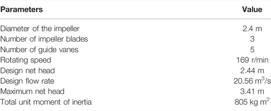
TABLE 1. Characteristic parameters of the pumping station.

FIGURE 1

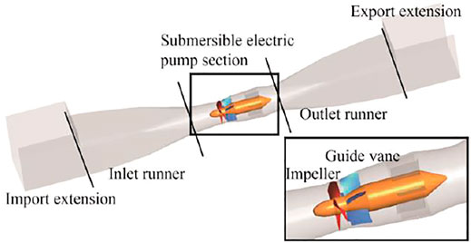
FIGURE 1. Three-dimensional model of the submersible tubular pump device.

Numerical Calculation Method

Turbulence Model

The numerical calculation is carried out based on ANSYS Fluent. The control equation is the incompressible Reynolds time-averaged equation:

$\frac{\partial \overline{u_i}}{\partial t}+\overline{u_j}\frac{\partial \overline{u_i}}{\partial x_j}=-\frac{1}{\rho }\frac{\partial \overline{p}}{\partial x_i}+\frac{{\mu }_t}{\rho }\frac{{\partial }^2\overline{u_i}}{\partial x_j\partial x_j}-\frac{\partial \overline{u_i^{\prime }{u}_j^{\prime }}}{\partial x_j},(1)$

where ρ is the density, u is the velocity, p is the pressure, and the subscripts i, j denote the directions of the Cartesian coordinates.

The turbulence model is the SST k–ω model. The SST k–ω model is modified by the standard k–ω model and the k–ε model. The model takes into account the near-wall performance of the k–ω model and the far-field accuracy of the k–ε model and can accurately predict the internal flow characteristics of the pump (Kent, 1954). The transport equations of turbulent kinetic energy k and specific dissipation rate ω in the SST model can be expressed as follows:

$\frac{\partial \rho k}{\partial t}+\frac{\partial }{\partial x_j}\left(\rho u_{j}k\right)=P_k-{\beta }^{\ast }\rho k\omega +\frac{\partial }{\partial x_j}\left[\left(\mu +\frac{{\mu }_t}{{\sigma }_k}\right)\frac{\partial k}{\partial x_j}\right]+P_{kb},(2)$

$\frac{\partial \rho \omega }{\partial t}+\frac{\partial }{\partial x_j}\left(\rho u_j\omega \right)={\alpha }^{\prime }\frac{\omega }{k}{P}_k-\rho \beta {\omega }^2+\frac{\partial }{\partial x_j}\left[\left(\mu +\frac{{\mu }_t}{{\sigma }_{\omega }}\right)\frac{\partial \omega }{\partial x_j}\right]+P_{\omega b},(3)$

The turbulent viscosity μ_t of the SST model is defined as

${\mu }_t=\frac{\rho {\alpha }_{1}k}{\max \left({\alpha }_1\omega ,S{F}_2\right)},(4)$

where P_k is the production rate of turbulence, ${\alpha }^{\prime }$, $\beta$, ${\beta }^{\text{∗}}$, ${\sigma }_k$, ${\alpha }_1$, and ${\sigma }_{\omega }$ are model constants, S is a module of the strain rate tensor, and F₁ and F₂ are mixed functions. SST k–ω model mixing function construction and constant value can be found in the study by Langtry and Menter (2009).

In unsteady calculations, by differencing the equations, the governing fluid dynamics equations can be solved for each time step. From the fluid domain calculations, the forces and moments acting on the reservoir are calculated by integrating the pressure on the surface.

Six-DOF Model

Knowing the forces and moments on the object, the motion of the object is calculated by the 6DOF model. The power-off process of the submersible tubular pump device is a process in which the impeller loses power and passively rotates under the action of water flow. 6DOF is used to simulate the movement of the impeller. The 6DOF model was first applied for the study of external ballistics and was established (Fowler et al., 1920) in the early 20th century, but it was not until the 1950s that R.H. Kent (Kent, 1954) from BRL (Ballistic Research Laboratory) and A.S. Galbraith also from BRL redefined rigid body trajectory systematically by the vector method, and the A.S. Galbraith study was not published. The 6DOF model simplifies the motion of the rigid body to the translation and rotation around the centroid and predicts the motion of the rigid body by numerically integrating the Newton–Euler motion equation. In the numerical solution process of Fluent, the force and moment acting on the rigid body are calculated according to the integral of surface pressure (Snyder et al., 2003). For the translational motion of the center of gravity, the control equation is solved in the inertial coordinate system:

$\dot{\overrightarrow{v}}=\frac{1}{m}{\displaystyle \sum \overrightarrow{f}},(5)$

where $\overrightarrow{v}$ is the velocity vector of the rigid body moving along the center, $\overrightarrow{f}$ is the force at the centroid, and m is the mass of the rigid body.

The rotational motion is more easily calculated in the body coordinate to avoid the change of inertial characteristics in the motion process:

$\frac{d{\overrightarrow{\omega }}_B}{dt}=L^{-1}\left({\displaystyle \sum {\overrightarrow{M}}_B-{\overrightarrow{\omega }}_B\times L{\overrightarrow{\omega }}_B}\right),(6)$

where ${\overrightarrow{\omega }}_B$ is the angular velocity vector, L is the inertia tensor, and ${\overrightarrow{M}}_B$ is the moment acting on the rigid body.

During the power-off process of the tubular pump, the motion of the impeller is mainly the rotational motion around the axis, and the translational motion is very small. During the power failure process of the tubular pump, the motion of the impeller is mainly the rotational motion around the axis, and the translational motion and rotational motion in other directions are very small. For the axial rotational motion, it can be calculated as follows:

$\frac{d{\overrightarrow{\omega }}_B}{dt}=L^{-1}{\displaystyle \sum {\overrightarrow{M}}_B}.(7)$

In case 1, the first-order display format adapted from the study by Kan et al. (2020) was used to solve the above differential equations, and the rotational speed ${\overrightarrow{\omega }}_B$ at time step k+1 is determined as follows:

${\overrightarrow{\omega }}_B^{k+1}={\overrightarrow{\omega }}_B^k+L^{-1}{\displaystyle \sum {\overrightarrow{M}}_B\mathrm{\Delta }t},(8)$

where $\mathrm{\Delta }t$ is the time step during calculation.

There is a large numerical error in the calculation of the first-order display format, and this error will accumulate, which makes the calculation result quite different from the actual result. Therefore, the fourth-order multi-point Adams–Moulton formula is used for numerical integration to determine the speed in case 2, which is an important classical algorithm for solving the initial value problem of differential equations and widely used in aviation and other fields. The algorithm is as follows:

${\overrightarrow{\omega }}_B^{k+1}={\overrightarrow{\omega }}_B^k+\frac{\mathrm{\Delta }t}{24}\left(9\frac{d{\overrightarrow{\omega }}_B^{\text{k}+1}}{dt}+19\frac{d{\overrightarrow{\omega }}_B^{\text{k}}}{dt}-5\frac{d{\overrightarrow{\omega }}_B^{\text{k}-1}}{dt}+\frac{d{\overrightarrow{\omega }}_B^{\text{k}-2}}{dt}\right).(9)$

Boundary Conditions and Numerical Methods

The system reference pressure is set to 1 atmospheric pressure, and the pressure inlet and pressure outlet conditions are adopted. The inlet relative pressure is set to 0 Pa, and the outlet relative pressure is the pressure corresponding to different head conditions. The impeller is the rotating domain, the axis z is the rotating axis, the initial speed of the impeller is 169 r/min, and the rest is the stationary domain. The inlet and outlet channels of the submersible tubular pump device, the wheel hub, the shell, and the guide vane of the impeller are applied without slip conditions, and the wall function is used in the near-wall area to adapt to the turbulence model. The dynamic mesh progressive transient calculation is adopted. The motion of the impeller is predicted by the 6DOF model, and the whole impeller domain is set as the motion domain. Similar to the sliding mesh method, the data transmission is realized through the interface before and after the impeller, and the deformation of the mesh is not involved in the movement of the impeller. The calculation time is the time when the impeller passes through 10 circles, and the impeller passes through 2° at each time step. The last circle is retained as the initial condition for the calculation of the power failure process of the pump device.

The runaway speed is usually checked according to the maximum head in the design of pump station, so the maximum head condition is selected for numerical calculation. The initial calculation state of the power-off process is H₀ = 3.41 m, Q₀ = 18.7 m³/s, n₀ = 169 r/min, M₀ = 45.2 kN m. The calculation time step of the power-off process is 0.001 s, even if the rotation angle of the impeller reaching the maximum speed within each time step does not exceed 2°, which meets the requirements of the rotor–stator interaction (RSI) (Choi and Moin, 1994; Naidu et al., 2019). To ensure convergence, iteration is 60 steps in each time step. The finite volume method is used to discretize the equations, the gradient discrete method in the equations is least squares cell-based, the pressure term is in the PRESTO format, and the convection term, turbulent kinetic energy, and dissipation rate are in the third-order Runge–Kutta format. The PISO algorithm, a non-iterative algorithm for solving coupled velocity and pressure, is used to solve the flow field equations simultaneously, and the interface is used to transfer information between different regions.

Meshing and Irrelevance Analysis

The block grid division strategy is adopted, in which the impeller and guide vane regions are divided by a hexahedral structured grid by Turbogrid. The block grid division strategy is adopted. Except for the bulb break, which is divided by unstructured grids, the rest of the calculation area is divided by structured grids. The grid parameter y⁺ is a dimensionless quantity (Fernholz and Finley, 1980) describing the distance from the first layer of grid to the wall, defined as

$y^{+}=\frac{\mathrm{\Delta }y\rho u^{\ast }}{\mu }=\frac{\mathrm{\Delta }y}{v}\sqrt{\frac{{\tau }_w}{\rho }},(10)$

where Δy is the height from the first layer of mesh to the wall, u^* is the friction velocity near the wall, μ is the fluid viscosity, v is the fluid kinematic viscosity, and τ_w is the wall shear stress.

Maintaining the same topological structure, the global maximum grid size is used to control the grid density of each computational domain, and the local grid of each computational domain is specially encrypted to ensure the quality of the grid. In this study, in the impeller and other main flow components, y⁺ is within 30, and y⁺ on the blade surface is shown in Figure 2, which basically meets the requirements of SST k–ω turbulence model for near-wall grid quality. Moreover, the orthogonality of most of the grid elements of the impeller and guide vane is above 0.9, and the element volume ratio is less than 20. When the head is 3.41 m, the whole flow channel is calculated, and the grid independence is detected with the flow and torque calculation results as the indexes. The calculation results are shown in Figure 3. When the grid is increased to more than 6.53 million, the flow and torque change tends to be stable. Using the grid convergence method GCI (Grid Convergence Index) recommended by Roache (2003), based on Richardson extrapolation theory, when the grid number is 6.53 million, the uncertainty of flow and torque is 2.1% and 1.3%, respectively, which meets the grid independence requirements. Considering the calculation time and calculation accuracy, the final calculation grid number is determined to be 6.53 million. The grid of the main components is shown in Figure 4.

FIGURE 2

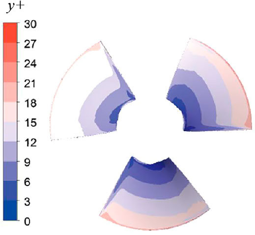
FIGURE 2. Distribution of y⁺ on the blade surface.

FIGURE 3

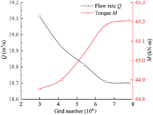
FIGURE 3. Grid independency test.

FIGURE 4

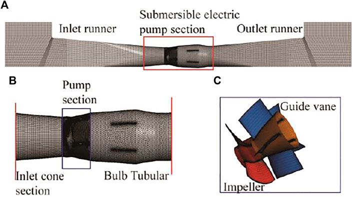
FIGURE 4. Three-dimensional model of the submersible tubular pump device: (A) pump unit; (B) submersible electric pump section; (C) pump section.

Figure 5 shows the comparison of energy characteristics between the numerical calculation and the experiment results under different flow conditions. It can be seen from the figure that affected by the solution accuracy, the Q–H curve obtained by numerical calculation is lower than the experimental result, which is mainly because the frozen rotor method is used in the steady simulation, and the relative position of the runner and the guide vane is fixed, which is different from the actual situation. However, in the entire calculation range, the numerical simulation results are basically consistent with the external characteristic relationship curve obtained from the experimental results. There is a certain deviation in the head under small flow conditions. This is mainly because the small flow conditions are close to the saddle area and the internal flow is more complicated, but the overall results are in good agreement, so the numerical simulation results can be considered to be highly reliable.

FIGURE 5

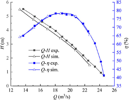
FIGURE 5. Comparison of the head and efficiency under different flow conditions.

Results and Discussion

Comparison of the Two Methods

Figure 6 shows the relative values of the external characteristic parameters of the submersible tubular pump device during the power-off process: n/n₀, Q/Q₀, and M/M₀ change with time. The entire power-off process can be divided into four stages: pump mode, braking mode, turbine mode, and runaway mode. At t = 0∼0.35 s, the pump works normally. The unit is powered off when t = 0.35 s, and the impeller and water flow still move in the original direction due to inertia. Due to the loss of power, the values of various parameters dropped rapidly. Compared with case 1, case 2 enters the braking mode earlier, and the braking condition lasts longer. When entering the hydraulic mode, the slope of the curve of case 1 is larger, that is, each parameter decreases faster than that of case 2 with time, so that the duration of the entire turbine mode is about 2s shorter than that of case 2. When the runaway condition is reached, the reverse speed and flow reach the maximum, the torque is zero, and the maximum runaway flow and maximum runaway speed of case 1 are higher than those of case 2.

FIGURE 6

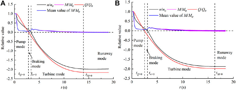
FIGURE 6. Relative values of dynamic parameter variations with time. (A) Case 1. (B) Case 2.

During the runaway test, the head is provided by the auxiliary pump, and the speed and flow rate are measured when the model pump device reverses and the output torque is zero under different heads. Runaway characteristics can be expressed by the unit speed n'_1,R and unit flow rate n'_1,Q, calculated as follows:

$n_{1,R}^{\prime }=\frac{n_{R}D}{\sqrt{H}},(11)$

$n_{1,Q}^{\prime }=\frac{Q_{R}D}{D^2\sqrt{H}},(12)$

where n_R and Q_R are the rotation speed and flow rate of the model pump device. The unit speed and unit flow rate of the model pump device are obtained from the test, and the rotation speed and flow rate of the prototype pump device in the runaway state under different head conditions can be obtained by conversion. Figure 7 shows the comparison of the calculation runaway rotation speeds and flow rates under different head conditions with the model test results. Under different heads, the runaway speeds calculated by case 1 and case 2 are larger than the test results, and case 2 is closer to the test results. This may be because the calculation ignores the friction torque of the radial bearing and the rotor wind resistance torque, and there is a certain deviation when the model is converted to the prototype itself. In general, the 6DOF model solved with the fourth-order multi-point Adams–Moulton formula has high accuracy in predicting the power failure process of the submersible tubular pump device. In case 2, t = 0∼2.5 s belongs to the pump condition; at this stage, the pump rotates in the forward direction and the water flow is in the forward direction. When t = 2.5 s, the fluid in the device is close to the transient static water body, i.e., Q/Q₀ =0. Until t = 3.1 s, the speed is zero. When t = 16.3 s, the reverse speed and flow reach the maximum, the torque is zero, the speed is about −1.88 times the initial speed, and the flow is about −1.98 times the initial flow. Compared with other pump device types, because the device is a similar straight pipe, the parameters of the unit drop faster when a power failure occurs, which is more harmful.

FIGURE 7

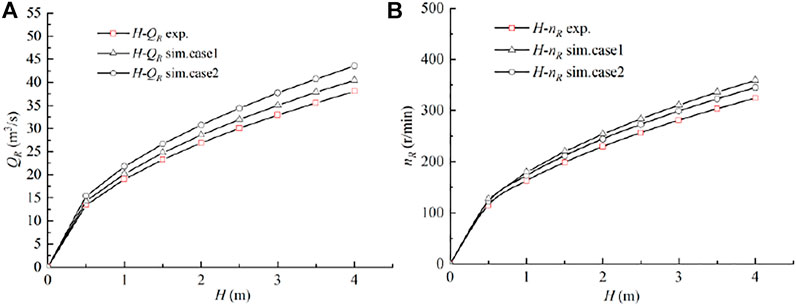
FIGURE 7. Comparison of the runaway rotation speeds (A) and flow rates (B) under different heads.

Analysis of Impeller Force

In the process of power failure, the water flow changes from forward flow to reverse flow. The changes in working conditions aggravate the asymmetry and unevenness of the flow field distribution in the pump. The uneven force on the pump body is likely to cause vibration and noise. Decompose the impeller force in the power-off process into two directions: axial force F_Z and radial force F_R. Define the dimensionless coefficient C_F as

$C_F=\frac{2F}{\rho U_t^{2}A},(13)$

where U_t is the circumferential velocity at the top of the impeller blade and A is the surface area of the blade. Figure 8 shows the variation curves of the impeller axial force coefficient C_FZ and the radial force coefficient C_FR calculated. As the working conditions of the unit change, the alternation of axial force and radial force gradually increases. The axial force of the unit presents a trend of gradual increase after a rapid decline over time, and the axial force varies greatly. The initial operating condition has the largest axial force coefficient, about 0.142, and the smallest axial force coefficient during the process is about 0.008, reaching a runaway operating condition of about 0.045. The radial force gradually increases with time, the average radial force coefficient increases from 0 to 0.004, and the radial force increases significantly.

FIGURE 8

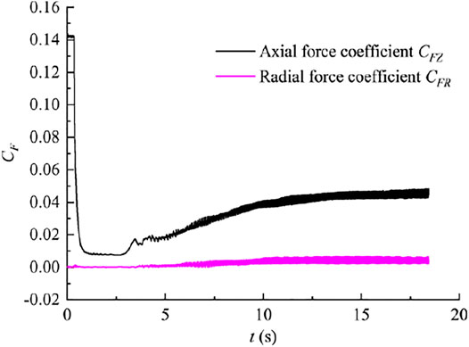
FIGURE 8. Force coefficient variations with time.

Internal Flow Field Analysis

Figure 9 is a longitudinal section pressure distribution and velocity streamline diagram of the submersible tubular pump device at the characteristic time. In the figure, the inlet of the left runner is the low-pressure side and the outlet of the right runner is the high-pressure side. When the unit is working normally, as shown in Figure 9A, the water flow is affected by the work done by the impeller and is from the low-pressure side to the high-pressure side. The streamline on the inlet side is straight, and the outlet side has multiple low-speed vortices propagating downstream due to the influence of the residual circulation of the guide vane outlet. When the unit is powered off, the functional power of the impeller drops rapidly. Under the action of the inlet and outlet pressure difference, part of the water flow starts to flow from the high-pressure side to the low-pressure side, and the vortex is formed by the collision of two water flows. When Q = 0, as shown in Figure 9B, the inside of the device is approximately still fluid, and a large range of vortices still remain from the streamline. There are also large vortices inside the bulb body, the motor of the submersible tubular pump device is located in the bulb body, and the generation of the vortex easily threatens the stability of the bulb body structure. When n = 0, as shown in Figure 9C, the reverse flow increases and the internal flow in the inlet channel is reformed, while the flow reformation of the outlet flow channel is relatively lagging, and there is still a certain vortex. Then, the unit enters the working condition of the turbine, and the increase of the reverse flow improves the flow pattern of the outlet flow channel, but at the same time, the accelerated rotation of the blades forms a vortex in the inlet flow channel. As shown in Figure 9D, in the runaway condition where the reverse flow rate and reverse rotation speed reach the maximum, the flow line in the outlet flow channel is smooth, and the inlet flow channel has a vortex similar to the draft tube of a hydraulic turbine propagating downstream.

FIGURE 9

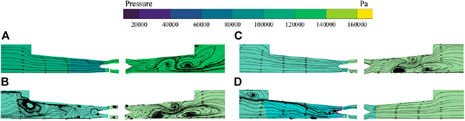
FIGURE 9. Streamline distribution and static pressure contours in the horizontal plane of the pump: (A) t = 0 s; (B) t =2.5 s; (C) t = 3.1 s; (D) t = 16.3 s.

Figure 10 shows the velocity streamline of the middle flow surface of the pump section at the characteristic time. When the pump is working normally, due to the deviation of the pump operating conditions from the design conditions, the vortex formed by flow separation is on the back of guide vane. When the forward flow rate is zero, the flow pattern in the middle flow surface is relatively chaotic. The water flow in the impeller is mainly in the circumferential direction, affected by the rotation of the impeller. There are also many vortices in the guide vane area, causing flow blockage. When the rotation speed is zero, the reverse flow of water flow improves the flow state in the guide vane, but due to the too large angle of attack of the water flow relative to the impeller, the flow separation occurs at the trailing edge of the blade. When the runaway condition is reached, the flow state of the intermediate flow surface is relatively good, and there is no obvious vortex.

FIGURE 10

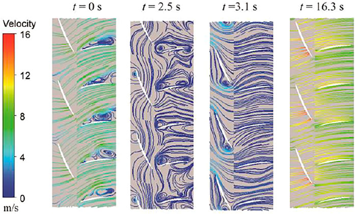
FIGURE 10. Distribution of velocity streamlines at medium span.

With the development of the power-off process of the pump device, the flow state of the pump inlet and outlet changes. Figure 11 shows the distribution of the velocity flow angle (the angle between the cross-sectional velocity and the circumferential velocity) at the impeller inlet, the impeller outlet, and the guide vane outlet at different times. When the pump is working normally (t = 0 s), the liquid flow angle at the inlet of the impeller is all around 90°, the water flow is approximately vertical inflow, and the liquid flow angle at the outlet of the impeller is greater than 90° due to the rotation of the impeller, and there is a backflow near the hub. The outlet of the guide vane is affected by the recovery circulation of the guide vane, which is similar to the vertical outflow, and there is also a de-flow at the hub. When the flow rate is 0 (t = 2.5 s), the velocity flow angle at about 3/4 of each section is negative, indicating that the water flow is reverse flow, and the negative liquid flow angle is distributed on the hub and rim side. With the development of time, the reverse flow is strengthened, and the outlet of the guide vane becomes the inlet of the water flow. When the rotation speed is 0, except for the recirculation area formed by the impact of the water flow on the shroud side of the guide vane outlet, the liquid flow angles of the impeller inlet and outlet sections are all negative values, and the flow is completely reverse flow. When t>2.5 s, the reverse rotation speed gradually increases with time, and the impeller’s intervention effect on the water flow is enhanced, which makes the inlet and outlet flow angles of the impeller tend to increase. The outlet of the guide vane is mainly affected by the reverse flow, and the recirculation area at the wheel rim gradually decreases.

FIGURE 11

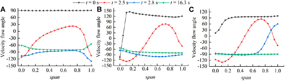
FIGURE 11. Distribution of the velocity flow angle at different times: (A) impeller inlet; (B) impeller outlet; (C) guide vane outlet.

Figure 12 is a cloud diagram of the blade surface pressure distribution at a characteristic time. When the pump is working normally, the pump pressure surface pressure is greater than that on the suction surface as shown in Figure 12A. The pressure distribution on the blade surface from the leading edge to the trailing edge shows a good gradient, the pressure on the pressure side shows a decreasing trend, while the suction side shows an increasing trend. As the positive flow rate decreases, part of the kinetic energy is converted into pressure energy. When the flow rate is zero, as shown in Figure 12B, there is no axial movement of water flow in the impeller, the pressure on the blade surface is uniformly distributed, and the pressure on the blade pressure surface and the suction surface pressure are almost equal. With the end of the pump condition, the reverse flow shock first causes the pressure in the local area of the blade pressure surface to increase, as shown in Figure 12C, which affects the stability of the blade structure. When the runaway condition is reached, as shown in Figure 12D, the angle of attack of the water flow relative to the blade airfoil is close to zero-lift, and there are a wide range of low-pressure areas on the suction surface of the blade.

FIGURE 12

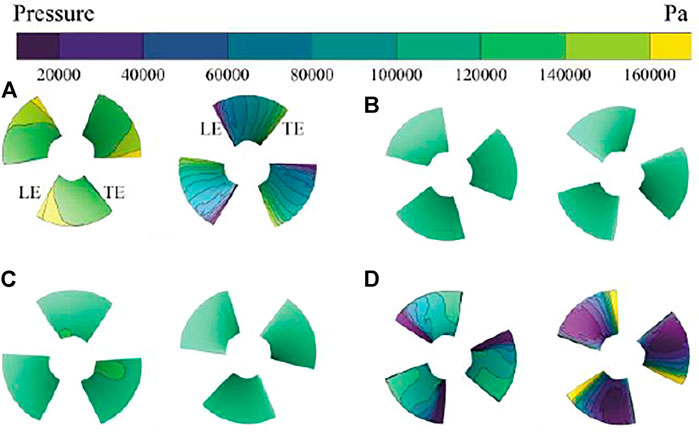
FIGURE 12. Pressure contours on blade pressure and suction surfaces at different times: (A) t = 0 s; (B) t =2.5 s; (C) t = 3.1 s; (D) t = 16.3 s. (The left side is the pressure side, and the right side is the suction side.).

Pressure Pulsation Analysis

In order to study the internal pressure pulsation of the pump unit during a power-off, monitoring points are set at the impeller inlet, impeller outlet, and guide vane outlet. The locations of the monitoring points are shown in Figure 13. Figure 14 shows the variation of pressure at the monitoring points with time. When the unit is working normally, the pressure surface and the suction surface have a large pressure gradient, which makes the pressure at the monitoring point in front of the impeller change regularly. When the unit is powered off, the speed of the water pump drops sharply, the forward flow velocity of the water flow decreases rapidly, causing the pressure at monitoring points P₁–P₃ before the impeller to rise until the forward flow is zero, and the average pressure in front of the impeller reaches the maximum value. Then, the reverse flow in the device increases, making the pressure in front of the impeller drop. As the pump enters the runaway condition, the reverse flow is the largest, and the average pressure at the monitoring point in front of the impeller reaches the minimum. The change of pressure at the monitoring points P₄–P₇ is the same as that at the monitoring point before the impeller when the unit is working normally. When the unit is powered off, the head of the impeller drops rapidly, the pressure of the water flowing through the impeller decreases rapidly, and the pressure at the monitoring points P₄–P₇ drops rapidly. The subsequent changes are similar to those of the monitoring points before the impeller. When the forward flow is the smallest, the average pressure reaches its maximum value and then continues to decrease. In the runaway condition, the average pressure reaches its minimum value. At the same time, the pressure fluctuations at the monitoring points are related to the speed of the impeller. The greater the speed, the greater the pressure fluctuation. At the same time, the pressure fluctuations before and after the impeller gradually decrease from the shroud to the hub. Compared with that at the monitoring points P₁–P₆, the pressure alternating at the monitoring point P₇ at the outlet of the guide vane is smaller due to the distance from the impeller.

FIGURE 13

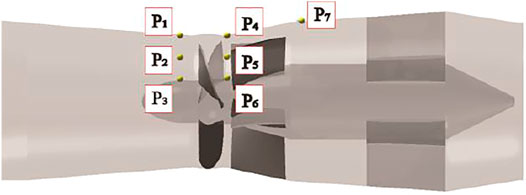
FIGURE 13. Pressure pulsation monitoring points.

FIGURE 14

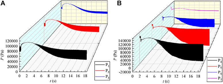
FIGURE 14. Time domain of the pressure fluctuation: (A) monitoring points P₁–P₃; (B) monitoring points P₄–P₇.

For further analysis of pressure pulsation, HHT (Hilbert–Huang transform) was used to process the pressure value. HHT is a new type of adaptive signal time–frequency processing method, which is different from STFT (short-time Fourier transform) and CWT (continuous wavelet transform). It does not require any basis function and is suitable for the analysis and processing of non-linear and non-stationary signals (Huang and Wu, 2008). The main content of HHT includes two parts: modal decomposition and Hilbert transform. Modal decomposition originally adopted EMD (empirical mode decomposition) (Huang et al., 1998; Wu and Huang, 2009), which was proposed by Huang. EMD is often referred to as a screening process. This screening process can decompose the complex signal into a finite number of IMFs (intrinsic mode functions), and each of the decomposed IMF components contains local characteristic signals of different time scales of the original signal. But when EMD decomposes the signal, there will be modal confusion, end effect, and curve problems. Therefore, VMD (variational mode decomposition) is used for modal decomposition in this paper (Dragomiretskiy and Zosso, 2014). VMD is an adaptive signal processing method; by iteratively searching for the optimal solution of variational mode and constantly updating each mode function and central frequency, several mode functions with a certain broadband are obtained. To remove edge effects, the algorithm extends the signal by mirroring half its length on either side. The second part is HT (Hilbert transform); the Hilbert transform of each IMF is obtained on the basis of VMD. Figure 14 shows the frequency spectrum of monitoring point P1 obtained by using HHT, STFT (window: kaiser), and CWT (wavename: Morlet). Figure 15 shows the frequency spectrum of monitoring point 1 obtained by using HHT, STFT (window: kaiser), and CWT (wavename: Morlet). The blade rotation frequency is defined as f_BRF = 3n/60. Compared with CWT and STFT, the time-spectrum frequency distribution obtained by HHT is more concentrated, all near the leaf frequency, avoiding the harmonic frequency (2 f_BRF, 3 f_BRF, etc.) components caused by the basis function of CWT and STFT.

FIGURE 15

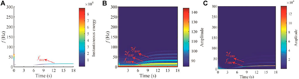
FIGURE 15. Spectrum analysis at monitoring point 1: (A) HHT; (B) STFT; (C) CWT.

Figure 16 shows the Hilbert spectrum obtained after HHT transformation. The blade rotation frequency is defined as f_BRF = 3n/60. The rotation speed of the impeller is the amount that changes with time, so the rotation frequency also changes with time. The instantaneous energy from the shroud to the hub shows a decreasing trend, which is consistent with the pressure fluctuation trend analyzed above. The main instantaneous energy of the monitoring points P₁–P₃ appears after about 6s, the frequency is concentrated around f_BRF, and the instantaneous energy gradually increases with time. The main instantaneous energy of the monitoring points P₄–P₆ also appears after 6 s, and the maximum instantaneous frequency is also concentrated around f_BRF. With the increase of flow and speed, high frequency components appear at monitoring points. The frequency component of monitoring points 4 and 5 is 2 f_BRF, 3 f_BRF, and 5 f_BRF, the guide vanes are 5, and 5 f_BRF are the frequencies due to static and dynamic interference. However, the frequency component of monitoring point P6 is 2 f_BRF, 3 f_BRF, and 4 f_BRF, and monitoring point 6 pressure is less affected by dynamic and static interference. The outlet of the guide vane has high pulsation energy when the pump is working normally, but when the power failure occurs, the monitoring point P7 pressure pulsation is weakened, and the main frequency is around 1 f_BRF and 2 f_BRF.

FIGURE 16

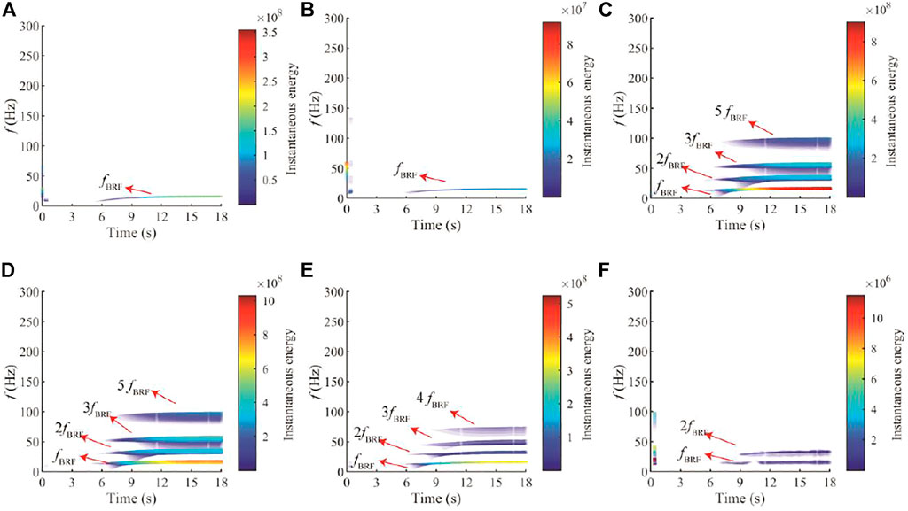
FIGURE 16. Hilbert spectrum of monitoring points: (A) P2; (B) P3; (C) P4; (D) P5; (E) P6; (F) P7.

Conclusion

Using a 6DOF model based on the fourth-order multi-point Adams–Moulton formula, this paper realizes the numerical simulation of the submersible tubular pump device during the power-off process and obtains the transient characteristics and internal flow characteristics of the unit’s operating parameter changes. It provides theoretical guidance for the stable operation of the pumping station, which has great engineering significance. The specific conclusions are as follows:

1. The 6DOF model based on the fourth-order multi-point Adams–Moulton formula has high accuracy for predicting the movement of the impeller during power failure. The results obtained using the fourth-order multi-point Adams–Moulton formula are more closer to the experimental values than the commonly used first-order display format.

2. In the process of power failure of the submersible tubular pump device, the flow of the pump device first changes from positive flow to reverse flow, and then the speed changes from positive to reverse. The interval from zero flow to zero speed is about 0.6 s. When the maximum head is 3.41 m, the speed is about −1.88 times the initial speed and the flow is about −1.98 times the initial flow.

3. The alternation of the axial force and radial force of the impeller gradually increases. The time-averaged axial force presents a trend of rapidly decreasing with time and then gradually increasing, while the radial force gradually increases with time, and the radial force coefficient increases significantly compared with the initial state.

4. In the process of power failure, there are a lot of vortices inside the device, especially when the flow is 0. There are also large vortices near the bulb body, and the generation of the vortex easily threatens the stability of the bulb body structure. There are also a large number of vortices in the impeller and guide vane. The impact of the reverse flow first causes the local pressure on the blade surface to increase, which threatens the stability of the blade structure.

5. The monitoring points at the inlet of the impeller show a trend of rising first and then falling with time. The monitoring points at the outlet of the impeller and the guide vane decrease rapidly when the power is turned off and then also show a trend of first rising and then falling with time. The pressure of each monitoring point is the highest near zero flow, and the pressure is the smallest at runaway. The main frequency of the pressure pulsation in the pump device is the blade pass frequency (f_BRF) and its harmonics, and the pressure pulsation intensity increases with the increase of the impeller speed.

Data Availability Statement

The raw data supporting the conclusion of this article will be made available by the authors, without undue reservation.

Author Contributions

ZS curated the data and wrote the original draft. FT performed formal analysis. JY reviewed and edited the paper. HG and HY were involved in project administration.

Funding

This project was funded by the Priority Academic Program Development (PAPD) of Jiangsu Higher Education Institutions.

Conflict of Interest

The authors declare that the research was conducted in the absence of any commercial or financial relationships that could be construed as a potential conflict of interest.

Publisher’s Note

All claims expressed in this article are solely those of the authors and do not necessarily represent those of their affiliated organizations, or those of the publisher, the editors, and the reviewers. Any product that may be evaluated in this article, or claim that may be made by its manufacturer, is not guaranteed or endorsed by the publisher.

References

Avdyushenko, A. Y., Cherny, S. G., Chirkov, D. V., Skorospelov, V. A., and Turuk, P. A. (2013). etcNumerical Simulation of Transient Processes in Hydroturbines. Thermophys. Aeromech. 20 (5), 577–593. doi:10.1134/s0869864313050059

CrossRef Full Text | Google Scholar

Chang, J. (2005). Transition Process of Hydraulic Mechanical Device. Higher Education Press.

Google Scholar

Choi, H., and Moin, P. (1994). Effects of the Computational Time Step on Numerical Solutions of Turbulent Flow. J. Comput. Phys. 113 (1), 1–4. doi:10.1006/jcph.1994.1112

CrossRef Full Text | Google Scholar

Dorfler, P. K. (2010). Improved Suter Transform for Pump-Turbine Characteristics. Int. J. Fluid Mach. Syst. 3 (4), 332–341. doi:10.5293/ijfms.2010.3.4.332

CrossRef Full Text | Google Scholar

Dragomiretskiy, K., and Zosso, D. (2014). “Variational Mode Decomposition,” in IEEE Transactions on signal Processing, February 1, 2014 (IEEE) 62, 531–544. doi:10.1109/TSP.2013.2288675

CrossRef Full Text | Google Scholar

Fernholz, H. H., and Finley, P. J. (1980). A Critical Commentary on Mean Flow Data for Two-Dimensional Compressible Turbulent Boundary Layers. Aerodynamics.

Google Scholar

Fowler, R. H., Gallop, E., and Lock, C. (1920). The Aerodynamics of a Spinning Shell. Proc. R. Soc. Lond. 98, 63. doi:10.1098/rspa.1920.0063

CrossRef Full Text | Google Scholar

Gou, D., Guo, P., and Luo, X. (2018). 3-D Combined Simulation of Power-Off Runaway Transient Process of Pumped Storage Power Station under Pump Condition. J. Hydrodynamics 33 (1), 28–39. doi:10.16076/j.cnki.cjhd.2018.01.004

CrossRef Full Text | Google Scholar

Guo, W., Zeng, W., and Yang, J. (2015). Runaway Instability of Pump-Turbines in S-Shaped Regions Considering Water Compressibility. J. Fluids Eng. Trans. ASME 137 (5), 051401. doi:10.1115/1.4029313

CrossRef Full Text | Google Scholar

Huang, N. E., Shen, Z., Long, S. R., Wu, M. C., Shih, H. H., Zheng, Q., et al. (1998). The Empirical Mode Decomposition and the Hilbert Spectrum for Nonlinear and Non-stationary Time Series Analysis. Proc. R. Soc. Lond. A 454, 903–995. doi:10.1098/rspa.1998.0193

CrossRef Full Text | Google Scholar

Huang, N. E., and Wu, Z. (2008). A Review on Hilbert-Huang Transform: Method and its Applications to Geophysical Studies. Rev. Geophys. 46 (2), 228. doi:10.1029/2007rg000228

CrossRef Full Text | Google Scholar

Jin, G., Pan, Z., and Meng, J. (2013). Study of the Runaway Character of Slanted Axial-Flow Pump. Chin. J. Hydrodynamics 5, 591–596. doi:10.3969/j.issn1000-4874.2013.05.012

CrossRef Full Text | Google Scholar

Kan, K., Chen, H., Zheng, Y., Zhou, D., Binama, M., and Dai, J. (2021). Transient Characteristics during Power-Off Process in a Shaft Extension Tubular Pump by Using a Suitable Numerical Model. Renew. Energy 164, 109–121. doi:10.1016/j.renene.2020.09.001

CrossRef Full Text | Google Scholar

Kan, K., Zheng, Y., Chen, H., Zhou, D., Dai, J., Binama, M., et al. (2020). etcNumerical Simulation of Transient Flow in a Shaft Extension Tubular Pump Unit during Runaway Process Caused by Power Failure. Renew. Energy 154, 1153–1164. doi:10.1016/j.renene.2020.03.057

CrossRef Full Text | Google Scholar

Kent, R. (1954). Notes on a Theory of Spinning Shell of Charge. Army Ballistic Research Lab Aberdeen Proving Ground MD.

Google Scholar

Langtry, R. B., and Menter, F. R. (2009). Correlation-based Transition Modeling for Unstructured Parallelized Computational Fluid Dynamics Codes. Aiaa J. 47 (12), 2894–2906. doi:10.2514/1.42362

CrossRef Full Text | Google Scholar

Li, W. (2012). Experimental Study on Transient Unsteady Internal Flow Characteristics of Inclined Flow Pump during Startup. Jiangsu University. Thesis.

Google Scholar

Li, Y., Zhu, Q., Liu, Z., and Yang, w. (2015). Numerical Simulation on Transient Characteristics of Double-Suction Centrifugal Pump System during Opening Valve Processes. Trans. Chin. Soc. Agric. Mach. 46 (12), 74–81. doi:10.1115/1.4002056

CrossRef Full Text | Google Scholar

Li, Z., Wang, L., and Dai, W. (2010). Diagnosis of a Centrifugal Pump during Starting Period Based on Vorticity Dynamics. J. Eng. Thermophys. 31 (1), 48–51.

Google Scholar

Liu, Y., and Chang, J. (2008). Numerical Method Based on Internal Character for Load Rejection Transient Caculation of a Bulb Turbine Installation. J. China Agric. Univ. 13 (001), 89–93. doi:10.11841/j.issn.1007-4333.2008.01.021

CrossRef Full Text | Google Scholar

Luo, X., Li, W., Feng, J., and Zhu, G. (2017). Simulation of Runaway Transient Characteristics of Tubular Turbine Based on CFX Secondary Development. Trans. Chin. Soc. Agric. Eng. 13, 97–103. doi:10.11975/j.issn.1002-6819.2017.13.013

CrossRef Full Text | Google Scholar

Menter, F. R., Kuntz, M., and Langtry, R. (2003). Ten Years of Industrial Experience with the Sst Turbulence Model. Heat Mass Transf. 4, 2814.

Google Scholar

Naidu, A., Oumer, A. N., and Azizuddin, A. A. (2019). Computational Fluid Dynamic (CFD) of Vertical-axis Wind Turbine: Mesh and Time-step Sensitivity Study[J]. J. Mech. Eng. Sci. 13 (3), 5604–5624. doi:10.15282/jmes.13.3.2019.24.0450

CrossRef Full Text | Google Scholar

Roache, P. J. (2003). Conservatism of the Grid Convergence Index in Finite Volume Computations on Steady-State Fluid Flow and Heat Transfer. J. Fluids Eng. 125 (4), 731–732. doi:10.1115/1.1588692

CrossRef Full Text | Google Scholar

Snyder, D., Koutsavdis, E., and Anttonen, J. (2003). “Transonic Store Separation Using Unstructured Cfd with Dynamic Meshing,” in 33rd AIAA fluid dynamics conference and exhibit, 23 June 2003 - 26 June 2003 (Orlando, Florida: AIAA), 3919. doi:10.2514/6.2003-3919

CrossRef Full Text | Google Scholar

Suter, P. (1966). Representation of Pump Characteristics for Calculation of Water Hammer. Sulzer Tech. Rev. 4 (66), 45–48.

Google Scholar

Wu, Z., and Huang, N. E. (2009). Ensemble Empirical Mode Decomposition: a Noise-Assisted Data Analysis Method. Adv. Adapt. Data Anal. 01 (01), 1–41. doi:10.1142/s1793536909000047

CrossRef Full Text | Google Scholar

Xu, H. (2008). Tubular Pumping Station. China Water&Power Press.

Google Scholar

Yang, F. (2013). Research on Hydrodynamic Characteristics of Low-Lift Pump Device and Key Technologies of Multi-Objective Optimization. Yangzhou university. Thesis.

Google Scholar

Yang, L., and Chen, N. (2003). Analysis of Relation between Characteristics of Pump-Turbine Runner and Transition of Pumped-Storage Power Station. J. Tsinghua Univ. Sci. Technol. 043 (010), 1424–1427. doi:10.16511/j.cnki.qhdxxb.2003.10.034

CrossRef Full Text | Google Scholar

Zeng, W., Yang, J., and Cheng, Y. (2015). Construction of Pump-Turbine Characteristics at Any Specific Speed by Domain-Partitioned Transformation. J. Fluids Eng. 137 (3), 031103. doi:10.1115/1.4028607

CrossRef Full Text | Google Scholar

Zhang, M. Y., Cheng, Y., Chen, F., Lu, T. L., Dong, Z. F., Pei, X. F., et al. (2014). 3D Cfd Simulation of the Runaway Transients of Bulb Turbine. Sichuan Da Xue Xue Bao Yi Xue Ban. 45 (5), 254–257. doi:10.15961/j.jsuese.2014.05.036

PubMed Abstract | CrossRef Full Text | Google Scholar

Zhang, X. X., Cheng, Y. G., Yang, J. D., Xia, L. S., and Lai, X. (2014). Simulation of the Load Rejection Transient Process of a Francis Turbine by Using a 1-D-3-D Coupling Approach. J. Hydrodyn. 26 (5), 715–724. doi:10.1016/s1001-6058(14)60080-9

CrossRef Full Text | Google Scholar

Zhou, D., Guo, Y., and Jiang, D. (2016). Numerical Simulation of Runaway Transients of Kaplan Turbine Model Based on Blade Regulation. Adv. Sci. Technol. Water Resour. 36 (4), 13–19. doi:10.3880/j.issn.1006-7647.2016.04.003

CrossRef Full Text | Google Scholar

Zhou, D., and Liu, Y. (2015). Numerical Simulation of Axial Pump Unit Startup Process Using Vof Model. J. Drainage Irrigation Mach. Eng. 34 (4), 307–312. doi:10.3389/fenrg.2021.706975

CrossRef Full Text | Google Scholar