A Data Driven Based Ultra Short PV Forecasting Method With Sky Images

Introduction

In recent years, the penetration level of renewable energy has increased rapidly to reduce carbon emissions and make the power grid more sustainable (Jiang et al., 2011). The cost of photovoltaic (PV) systems is reducing rapidly. PV systems are replacing conventional coal-fired power plants with a lower cost per kWh. Owing to the replacement effects of fully controllable coal-fired power plants with partially controllable PV resources, the need for dispatchable operational resources will significantly increase the operating cost of power systems and bring significant challenges (Ipakchi and Albuyeh, 2009; Farhangi, 2010; Huang et al., 2011). Power fluctuations and the unavoidable randomness of renewable energy require a large capacity for flexible operating resources and spinning reserves (Grainger et al., 2014). All controllable operating resources must be coordinated effectively to overcome these challenges. As a result, forecasting methods for PV systems are essential for such tasks. The forecasting methods of PV systems include several time scales, including long-term, day-ahead, short-term, and ultra-short-term. The short and ultra-short PV forecast results can be integrated into the optimal power flow models to determine the optimal set points for the generators. Based on the updated forecast results with higher accuracy, the operation costs of the system can be reduced and the negative effectiveness of output power fluctuations can be reduced. Moreover, such forecast results can be used to determine the on/off status of quick response resources, such as gas turbines, demand response devices, and energy storage systems. In this way, PV systems with controllable resources can enhance the power supply for critical loads after extreme natural disasters. Thus, the resilience of power systems can be enhanced by accurate PV forecast results (Liang et al., 2017).

Currently, there are several methods for implementing an ultra-short PV forecast system including statistical, physical, and hybrid methods (Liu et al., 2015). In this study, a hybrid-type ultra-short PV forecast method is proposed to predict the average output power of PV systems for the following 5 min. Historical data, cloud information, and data from PV systems are used to determine the output power of PV systems.

For ultra-short PV forecast methods, which use physical and hybrid methods, cloud is one of the major factors determining the output power (Wan et al., 2015). Fu et al. (2021) proposed an improved convolutional autoencoder-based sky image prediction model to improve the feature extraction ability. Zhen et al. (2019) proposed a method based on particle swarm optimization to calculate the speed of clouds. The effects of clouds on solar irradiance could then be calculated knowing the accurate speed of the clouds. With the development of artificial intelligence (AI) technologies, the image processing capability has improved greatly. Consequently, several different AI networks are used to process sky images (Zhen et al., 2020; Wen et al., 2021; Zhang et al., 2021). In these studies, sky images were processed by deep learning and bidirectional long short-term memory (Bi-LSTM) networks for PV forecast systems. A Bi-LSTM network is a type of LSTM network with bidirectional capability. LSTM networks were first proposed by Hochreiter and Schmidhuber in 1997 (Hochreiter and Schmidhuber, 1997). The LSTM network has been improved with new features and better performance in recent years (Gers et al., 2000; Cho et al., 2014; Greff et al., 2017). A Bi-LSTM network was selected for the current study, to determine the output power for PV systems with several different features. In (Zhang et al., 2019), a PV forecasting method was proposed to determine the output power of the whole PV station with time based analog ensemble method. In (Yan et al., 2021), a deep learning network was applied with frequency-domain data to predictive the ultra-short-term output power of PV systems.

Image processing algorithms, such as speeded up robust features (SURF), fast library for approximate nearest neighbors (FLANN), and Gabor filters, have been proposed and improved to enhance image processing capabilities in recent years (Grigorescu et al., 2003; Bay et al., 2008; Muja and Lowe, 2014). In this study, the features of sky images were extracted and processed with SURF, FLANN, and Gabor filter methods.

The major contributions of this study can be summarized as follows:

1) A processing method combined with SURF, FLANN, and Gabor filters was proposed to calculate the brightness of the radiation from the key area, which was an important factor for predicting the output power of PV systems for the following few minutes.

2) A Bi-LSTM network was proposed to predict the output power of PV systems using the different features extracted from sky images, hardware systems, and historical data.

3) A testbed system was set up to capture the sky images and verify the proposed ultra-short PV forecast method.

This paper is organized as follows: The framework and methods for feature extraction of the proposed PV forecasting methods are described in the next section followed by a description of the intelligent network and data flows. The calculations made are then broken down into their constituent parts, and finally a case study is described.

Ultra-Short Forecasting Method Framework

As shown in Figure 1, the framework of the proposed ultra-short PV forecasting method includes two parts. First, several key features were extracted from sky images, historical data, and hardware systems. The features extracted from the sky images include the brightness of the key area, cloud coverage, and cloud texture type. The historical data, temperatures, and incident and elevation angles of the PV system were obtained from the PV system hardware. These results were then fed into a Bi-LSTM network to calculate the output power of the PV system for the following 5 min.

FIGURE 1

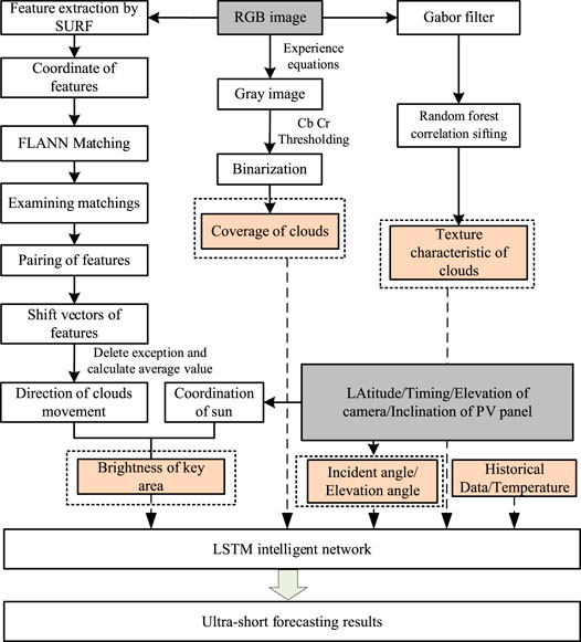
FIGURE 1. Framework of the proposed ultra-short PV forecasting method.

In this study, for all the features obtained from the physical hardware system and the images in real time, the LSTM network was used to determine the PV output power. The structure of a typical LSTM is shown in Figure 2A.

FIGURE 2

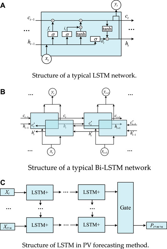
FIGURE 2. Structure of a typical LSTM, Bi-LSTM network and the LSTM in PV forecasting method. (A) Structure of a typical LSTM network. (B) Structure of a typical Bi-LSTM network. (C) Structure of LSTM in PV forecasting method.

The LSTM includes collecting, selecting, and generating information. It can be modeled as follows (Greff et al., 2017),

$f_t=\sigma \left(W_f\cdot \left[h_{t-1},x_t\right]+b_f\right)(1)$

$i_t=\sigma \left(W_i\cdot \left[h_{t-1},x_t\right]+b_i\right)(2)$

$o_t=\sigma \left(W_o\cdot \left[h_{t-1},x_t\right]+b_o\right)(3)$

$c_t=f_t{c}_{t-1}+i_t\tanh \left(W_c\cdot \left[h_{t-1},x_t\right]+b_c\right)(4)$

$h_t=o_t\tanh \left(c_t\right)(5)$

$y_t=W_y\cdot \left[c_t,h_t\right]+b_y(6)$

Based on a typical LSTM, the Bi-LSTM network was developed to consider the information in the future. The structure of a typical Bi-LSTM is shown in Figure 2B (Siami-Namini et al., 2019).

A Bi-LSTM consists of both a forward and a backward network. A network structure based on LSTM and Bi-LSTM networks was proposed in this study to predict the output power of PV systems in the near future, as shown in Figure 2C.

Based on the proposed Bi-LSTM structure, all features of the PV forecasting-related data were imported to train the LSTM network and obtain the forecasted results.

Calculation of Cloud Coverage

Clouds can affect the radiation of the sunshine on the PV systems, thereby reducing the output power. The cloud coverage affects the brightness of radiation striking the PV system cells, and therefore needs to be quantified. Normally, cloud coverage can be obtained from the local observatory with a time interval of 1 h. The ultra-short-term PV forecasting method cannot support a time resolution of 1 h. Consequently, sky images in real time from satellites and cameras were used to calculate the cloud coverage in real time. When the sky images from both satellites and cameras are available for the PV forecast method, the accuracy of the forecast results can be improved. However, satellites may not be available for all PV systems to provide the required sky images in real time. A camera is therefore a good choice for providing local sky images for PV systems. If the satellites Sky images captured by cameras are in RGB format. The RGB image can be converted into a gray image using the experience equation:

$GI\left(i,j\right)={\alpha }_{r}R\left(i,j\right)+{\alpha }_{g}G\left(i,j\right)+{\alpha }_{b}B\left(i,j\right)(7)$

where i and j are the pixel coordinates in the RGB image. The $GI\left(i,j\right)$ function represents the gray value of the pixel. The $R\left(i,j\right)$, $G\left(i,j\right)$, and $B\left(i,j\right)$ functions represent the values of the red, green, and blue colors, respectively, of the pixel. The ${\alpha }_r$, ${\alpha }_g$, and ${\alpha }_b$ are the coefficients of the three colors used to calculate the gray value of the pixel.

As shown in Figure 3, original RGB images are shown in Figure 3A. The gray images obtained using Eq. 7 of the original images are shown in Figure 3B. The 3D gray distributions for these images are shown in Figure 3C. Based on these results, pixels for different locations and weather conditions can be recognized by the gray values. For most days, the pixel gray values around the sun, of blue sky, and of clouds are 220–255, 50–120, and 100–240, respectively.

FIGURE 3

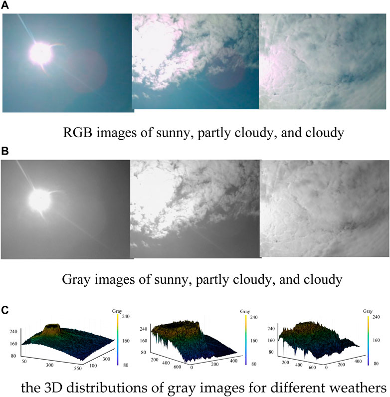
FIGURE 3. Results of sky images for different cloud coverage. (A) RGB images of sunny, partly cloudy, and cloudy. (B) Gray images of sunny, partly cloudy, and cloudy. (C) The 3D distributions of gray images for different weathers.

To calculate cloud coverage, the gray image was converted into a binary image. This process is called binarization:

$BI\left(i,j\right)=\{\begin{array}{cc}0& GI\left(i,j\right)<\delta \\ 1& GI\left(i,j\right)\ge \delta \end{array}(8)$

where BI(i,j) is the binary value of pixel (i,j) of the image, and $\delta$ represents the binarization threshold. For the binary results, the cloud coverage can be calculated as follows:

$CV=\frac{{\displaystyle \sum _{i,j}^{m,n}BI\left(i,j\right)}}{m\times n}(9)$

where CV is the cloud coverage, and m and n represent the dimensions of the image. As shown in Figure 3B, the gray values of the clouds far away from the sun are lower than those of the sky near the sun. As a result, the binarization method described in Eqs 8, 9 cannot recognize clouds from images and cannot calculate the cloud coverage accurately.

Air has a stronger scattering effect on blue than on other colors while clouds have equivalent scattering effects on all colors. The difference in the scattering effects can be imported to improve the accuracy of the binarization. First, the coordinates of the sun, x₀, and y₀, can be calculated according to the sky image and time of day. The factor $\text{γ}\left(i,j\right)$ can then be calculated as follows:

$\gamma \left(i,j\right)=\frac{\sqrt{{\left(x_0-i\right)}^2+{\left(y_0-j\right)}^2}}{\max \left(d_{ij}\right)}(10)$

where max (d_ij) represents the maximal distance of all pixels to the center of the sun on the image, as shown in Figure 4. To recognize the clouds and the sky near the sun, the ratios of blue and red colors are used to improve the accuracy of calculating cloud coverage. The binarization can be calculated as:

$BI\left(i,j\right)=\{\begin{array}{cc}0& R\left(i,j\right)/B\left(i,j\right)<R{B}_T\left(1-\gamma \left(i,j\right)\right)\\ 1& R\left(i,j\right)/B\left(i,j\right)\ge R{B}_T\left(1-\gamma \left(i,j\right)\right)\end{array}(11)$

where RB_T represents the threshold for binarization. In most cases, the R/B ratio of sun and clouds nearby are around 1.0 while the R/B ratio of the clear sky will decrease from 1.0 to 0.4 with increasing distance. Consequently, the distance and color factors are considered in Eq. 11 to improve the accuracy of binarization.

FIGURE 4

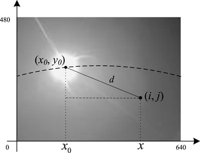
FIGURE 4. Calculating factor γ from the coordinates of sun.

The binarization results with the original and improved methods are shown in Figures 5A–H. As indicated in Figures 5D,H, the improved method described in Eqs 10, 11 could improve the accuracy of binarization and cloud coverage.

FIGURE 5

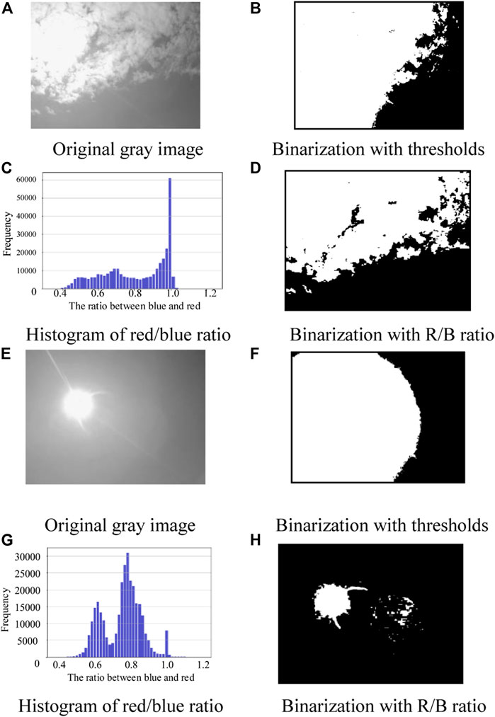
FIGURE 5. Calculating cloud coverage by binarization. (A) Original grey image. (B) Binarization with thresholds. (C) Histogram of red/blue ratio. (D) Binarization with R/B ratio. (E) Original gray image. (F) Binarization with thresholds. (G) Histogram of red/blue ratio. (H) Binarization with R/B ratio.

Calculation of Key Area Brightness

The brightness of radiation striking the PV panel is the key factor in determining the output power of PV systems. The brightness of an area is defined as follows:

$\text{Br}=\frac{{{\displaystyle \sum }}_{i,j}^{m,n}GI\left(i,j\right)}{m\times n}(12)$

The brightness is directly related to the radiation striking the PV panel and determines the output power of the PV system. For the ultra-short PV forecasting method, both the position of the sun and the direction of cloud movement need to be considered to calculate the brightness of a specific area. The position of the sun is associated with time, latitude, and longitude. In the early morning and late afternoon, the sun may not appear on the images captured by the camera in real time. Considering that the output power of the PV panel is relatively low, the position of the sun can be ignored, and the brightness can be calculated using Eq. 12. The speed and direction of clouds are also considered in ultra-short PV forecasting methods. The wind speed on the ground is different from the wind speed near the clouds and cannot be used to calculate the speed of clouds. Images of clouds in real time can however be used to calculate such cloud information.

Feature Recognition

In this study, the classical SURF method was used to recognize the features of clouds. The Hessian matrix of an image can be calculated as:

$H\left(f\left(x,y\right)\right)=\left(\begin{array}{cc}\frac{{\partial }^{2}f\left(x,y\right)}{\partial x^2}& \frac{{\partial }^{2}f\left(x,y\right)}{\partial x\partial y}\\ \frac{{\partial }^{2}f\left(x,y\right)}{\partial x\partial y}& \frac{{\partial }^{2}f\left(x,y\right)}{\partial y^2}\end{array}\right)(13)$

where f (x,y) is the convolution of pixels (x,y) with a Gaussian function. The results of filtering using $\text{σ}$ can be represented as:

$H\left(x,\sigma \right)=\left(\begin{array}{cc}{L}_{xx}\left(x,\sigma \right)& L_{xy}\left(x,\sigma \right)\\ L_{xy}\left(x,\sigma \right)& L_{yy}\left(x,\sigma \right)\end{array}\right)(14)$

$\{\begin{array}{l}{L}_{xx}\left(x,\sigma \right)=\frac{{\partial }^2\left(g\left(\sigma \right)I\right)}{\partial x^2}\\ L_{xy}\left(x,\sigma \right)=\frac{{\partial }^2\left(g\left(\sigma \right)I\right)}{\partial x\partial y}\\ L_{yy}\left(x,\sigma \right)=\frac{{\partial }^2\left(g\left(\sigma \right)I\right)}{\partial y^2}\end{array}(15)$

The SURF algorithm replaces the L_xx, L_xy, and L_yy operators using box filters. The sign of det(H) is used to determine if pixel (x,y) is a feature point in the image. When the Hessian matrix is a positive or negative definition, the pixel (x,y) is recognized as a feature point. The results of the SURF algorithm are shown in Figure 6.

FIGURE 6

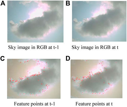
FIGURE 6. Recognition results with SURF algorithm. (A) Sky image in RGB at t-1 (B) Sky image in RGB at t. (C) Feature points at t-1 (D) Feature points at t.

FLANN for Feature Matching

In this study, FLANN with a k-dimensional (KD) tree was used to match the features for images, which reduced the search time and improved the efficiency, compared with the conventional FLANN searching method. The matching method is shown in Figure 7.

FIGURE 7

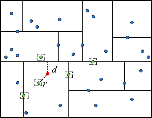
FIGURE 7. FLANN searching method with KD tree.

First, a KD tree is constructed with all the feature points. The KD tree consists of several branches that contain different feature points. The red point in Figure 7 corresponds to the point to be matched. The nearest point to the red point in the same branch is found, and the distance is marked as r. The distances between the red point and other branches, d_i, are then calculated. If d_i > r, the calculations for all points located in branch i can be skipped. Moreover, a factor α can be imported to accelerate the search process. The condition d_i > r can be revised to d_i > r/α.

Identifying Mismatching of FLANN

The results of the feature matching include numerous errors. The points of mismatching need to be identified and removed to calculate the direction and speed of cloud movements. Both the best and second-best matching points were recorded for the FLANN method. Normally, the distance to the best point is much smaller than that to the second-best point. The ratio between these two distances can be used to determine if the best matching point is the correct matching result. The identification method is described as:

$\sqrt{{\displaystyle \sum _{i=1}^n{\left(a_i-b_i\right)}^2}}<\eta \sqrt{{\displaystyle \sum _{i=1}^n{\left(a_i-b_i^{\prime }\right)}^2}}(16)$

where a_i is the feature point to be matched, and b_i and $b_i^{\prime }$ are the best and second-best matching points, respectively. The best matching point is the correct matching point when Eq. 16 is satisfied.

In this way, the moving direction and speed of clouds can be calculated using the difference between these matching feature points in two images. Based on the calculated distance difference of these feature points, the 3σ criteria can be used to delete the invalid points as follows:

$\sigma =\sqrt{\frac{1}{n}\left({\displaystyle \sum _1^n{\left(x_i-\overline{x}\right)}^2}\right)},\left|x_i-\overline{x}\right|>3\sigma (17)$

If the distance between these two images is larger than 3σ, the point is removed from the calculation of the moving direction and speed of clouds. The moving direction and speed of the clouds can then be calculated based on the set of feature points.

Key Area Brightness

The key area is defined as the area that is closer to the sun in the next time interval of the forecast system. In this study, the PV forecast system determined the output power of the PV system in the following 5 min. If the sun is visible, the rectangular area that is moving towards the center of the sun is defined as the key area, as shown in Figure 8A. When the sun is not visible in the sky, a circular area at the center of the image is selected as the key area, as shown in Figure 8B.

FIGURE 8

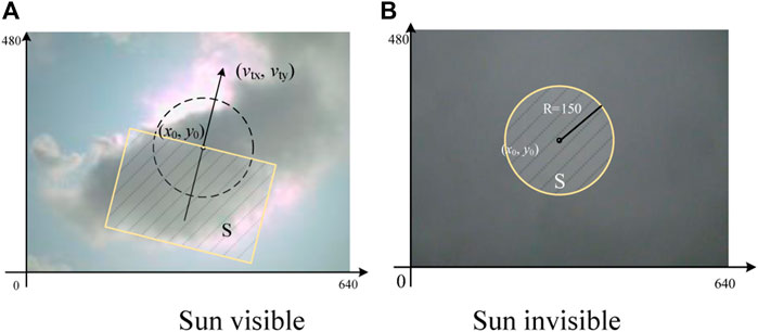
FIGURE 8. Definition of key area. (A) Sun visible (B) Sun invisible.

Texture Feature of Clouds

Cloud coverage only indicates the percentage of the visible sky that contains clouds. The types of clouds also affect the brightness of the radiation striking the PV panel and the output power of the PV system. Some typical clouds include cumulus clouds, cirrus clouds, stratocumulus, and cumulonimbus, as shown in Figure 9.

FIGURE 9

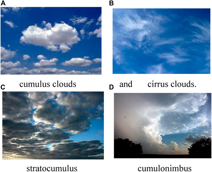
FIGURE 9. Typical types of clouds. (A) cumulus clouds and (B) cirrus clouds. (C) stratocumulus (D) cumulonimbus.

The reduction effect of cirrus clouds on the brightness of the sun is normally weak owing to the cloud height. The cumulus clouds and stratocumulus could greatly reduce the brightness of the sun owing to the shape and thickness of these clouds. In this way, identifying the type of cloud is important for evaluating the output power of PV systems. In this study, the Gabor filter is used to identify the features of different types of clouds.

$g_{\lambda ,\theta ,\phi ,\sigma ,\gamma }\left(x,y\right)=\exp \left(-\frac{x^{\text{′}2}+{\gamma }^2{y}^{\prime 2}}{2{\sigma }^2}\right)\exp \left(i\left(2\pi \frac{x^{\prime }}{\lambda }+\phi \right)\right)(18)$

$x^{\prime }=x\cos \theta +y\sin \theta (19)$

$y^{\prime }=-x\sin \theta +y\cos \theta (20)$

where λ is the wavelength of the sinusoidal factor (θ) in the Gabor filter, which is normally between 2 pixels and 1/5 of the entire image; θ represents the angle of the Gabor function; σ represents the standard deviation of the Gaussian function in the Gabor filter; γ represents the aspect ratio of the ellipse in the Gabor function; and φ represents the phase angle of the cosine function. The energy, average, and standard deviation of each image are chosen as the major features to describe the images as follows:

$E_{\theta ,\lambda }={\displaystyle \sum _{i,j}^{M,N}{G}_{\theta ,\lambda }{\left(i,j\right)}^2}(21)$

$m_{\theta ,\lambda }=\frac{1}{MN}{\displaystyle \sum _{i,j}^{M,N}{G}_{\theta ,\lambda }\left(i,j\right)}(22)$

$S_{\theta ,\lambda }=\frac{1}{MN}{\displaystyle \sum _{i,j}^{M,N}{\left(G_{\theta ,\lambda }\left(i,j\right)-m\right)}^2}(23)$

For different combinations of λ_i and θ_j, the Gabor filter can generate i × j results. The random forest regression method was then imported to select these results. The detailed procedure includes the following steps.

1) Normalization of eigenvectors.

2) Build regression tree with a single feature.

3) Model assessment.

4) Enumerate all features by repeating steps (2) and (3). Calculate the results of the evaluation index for all the features.

5) Select the features according to the results of the evaluation index.

Case Studies

In the case studies, the Bi-LSTM network includes a 4-layer structure. The number of cells in the feedforward network was set to 50. The PV forecasting system can determine the output power of the PV system in the following 5 min with a 10 s time interval. 24 PV panels each with a 230 W rated power capacity were installed as the PV system. The total power capacity of the PV system was therefore 5520 W. The resolution of the camera was 480 × 640 pixels. The OpenCV toolbox was used to calculate the features of the captured images.

PV Forecasting System Hardware

The PV forecasting system hardware is shown in Figure 10A, and the installation angles are shown in Figure 10B $\gamma =19.44°$ and $\beta =49°$ for the experimental system. The PV system was located at the Xili University Town of Shenzhen, with a latitude of $\mathrm{22}\mathrm{.591}°$. The relationships between the incident and elevation angles with time are shown in Figure 11. The details of temperature are shown in Figure 12. In this way, the incident and elevation angles were calculated as 21.602° and 58.739°, respectively. A camera was installed with the PV panels. The actual active output power of the PV system was collected through the RS 485 port from the power inverter of the PV system. The temperature was collected from a local meteorological station.

FIGURE 10

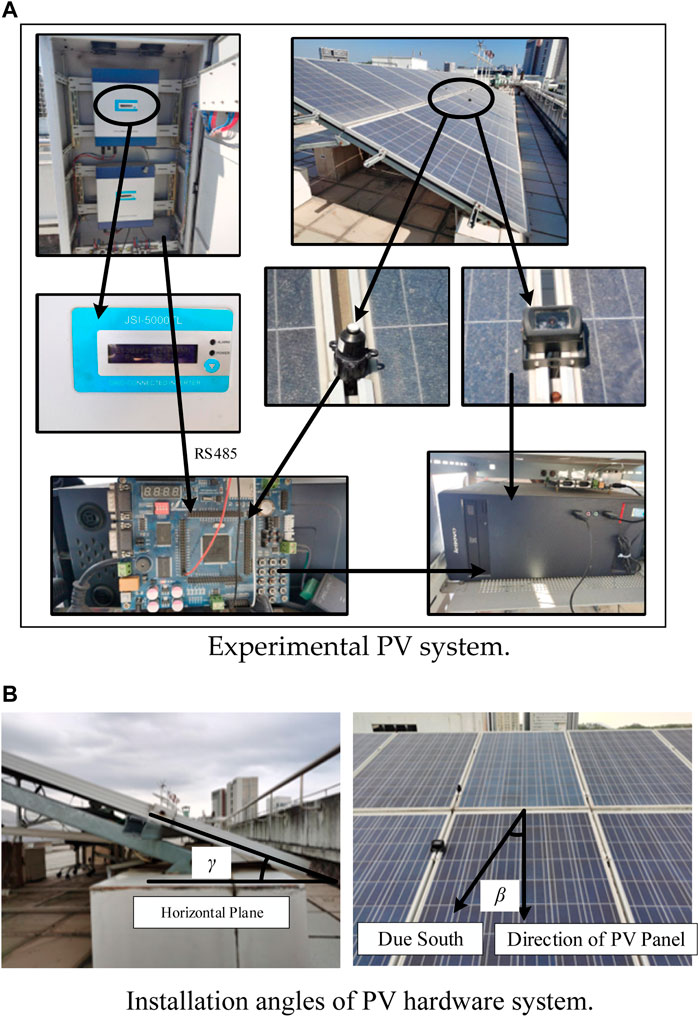
FIGURE 10. Details of PV hardware system. (A) Experimental PV system. (B) Installation angles of PV hardware system.

FIGURE 11

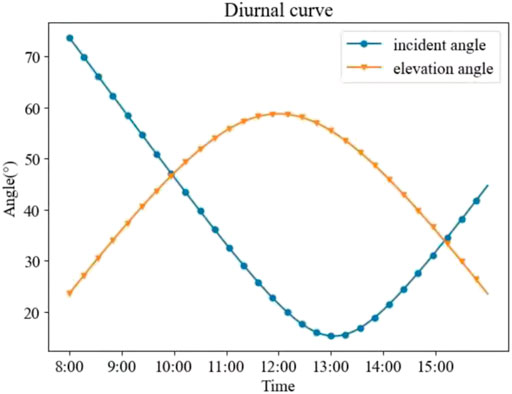
FIGURE 11. Incident and elevation angles as a function of time.

FIGURE 12

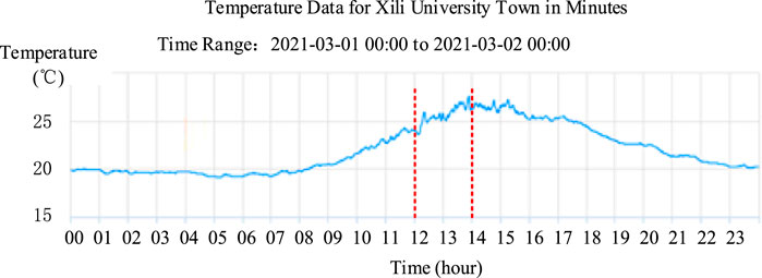
FIGURE 12. Temperature at different times at Xili University Town.

PV Forecasting System Data Flow

The data flow of the proposed PV forecasting system is illustrated in Figure 13. The features of the clouds and brightness were obtained from the images captured by the camera in real time. The temperature, and incident and elevation angles were collected from the local meteorological station and goniometers. The input vector X_t can be generated based on the information at time t. The output vector Y_t consists of the active output power of the PV system collected from the power converter. The input vectors were first normalized. Then, the vectors were imported to train the network. Finally, the forecast results in the following time intervals were generated by the network.

FIGURE 13

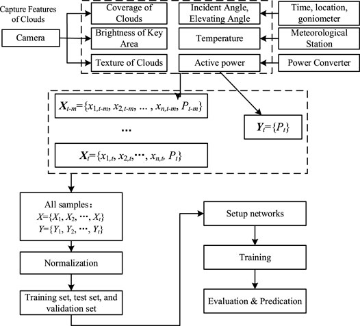
FIGURE 13. Data flow of PV forecasting system.

Normally, the stochastic gradient descent (SGD) and the adaptive moment estimation (ADAM) methods can be used to train the network. The SGD method can be described as follows:

$g_t=\nabla {\theta }_{t-1}f\left({\theta }_{t-1}\right)(24)$

$\mathrm{\Delta }{\theta }_t=-\eta g_t(25)$

ADAM increases the first- and second-order moment expressions compared with SGD as follows:

$g_t=\nabla {\theta }_t{f}_t\left({\theta }_{t-1}\right)(26)$

$m_t={\beta }_1\text{g}{m}_{t-1}+\left(1-{\beta }_1\right)g_t(27)$

$v_t={\beta }_2\text{g}{v}_{t-1}+\left(1-{\beta }_2\right)g_t^2(28)$

$\mathrm{\Delta }{\theta }_t=-\alpha \text{g}\frac{m_t}{\left(\sqrt{\frac{v_t}{1-{\beta }_2^t}}+\epsilon \right)\left(1-{\beta }_1^t\right)}(29)$

Sometimes, the ADAM method can achieve better results for training the network.

FLANN Feather Matching

As illustrated above, the FLANN method was applied to match the features with two images captured with a 10 s time interval. The matched features were used to calculate the speed and movement direction of the clouds. The features were first matched by the FLANN method and then identified by the proposed method in Eq. 17. The results are shown in Figure 14A and Figure 14B as follows:

FIGURE 14

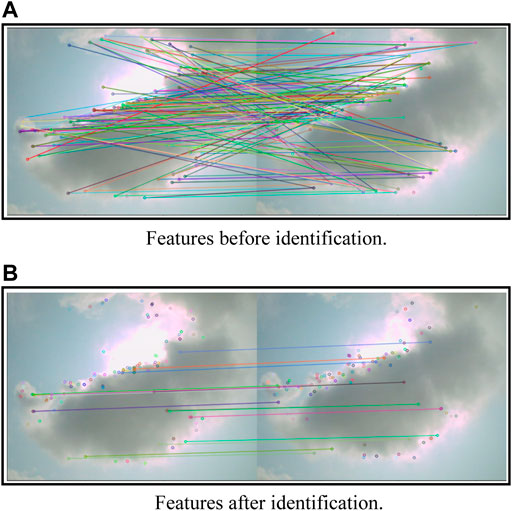
FIGURE 14. Features before and after identification. (A) Features before identification. (B) Features after identification.

The matching features are listed in Table 1. According to Eq. 17, some unusual feature points can be identified and deleted. The results are shown in Figure 14B. Based on these features, the moving vector of the clouds can be calculated as (4.5, 20.8).

TABLE 1

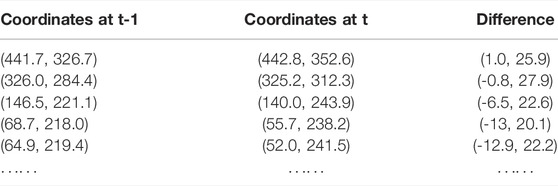
TABLE 1. Matched features in two images.

Cloud Texture Feature

The image shown in Figure 15A was applied to extract the features of textures with Gabor filters. The filtered results are shown in Figure 15B with wavelengths λ = 7, 15, and 23 in each column, respectively, and θ = 5°, 10°, 35°, and 45° in each row, respectively. Detailed calculation results with different indices are shown in Table 2.

FIGURE 15

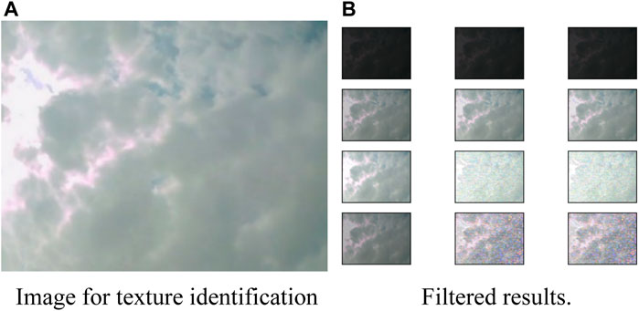
FIGURE 15. Filtered results with Gabor filters. (A) Image for texture identification (B) Filtered results.

TABLE 2

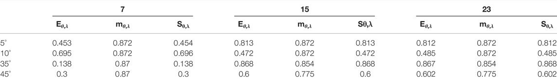
TABLE 2. Filtered results with gabor filters.

The results for λ = 15, θ = 35°, and λ = 23, and θ = 5° were selected as the features for the PV forecasting system in this study.

Finally, the data including several different features, as shown in Figure 16, were generated to train the Bi-LSTM network with the alternating direction method of multipliers algorithm. The forecast results were obtained using the trained Bi-LSTM network. The actual output power and forecasting results with different networks and data are presented in Figure 17A. The red line indicates the actual output power of the PV system. The green line indicates the forecasting results of the Bi-LSTM without cloud information. The orange and blue lines indicate the forecasting results with cloud information from the LSTM and Bi-LSTM networks, respectively. This indicates that the Bi-LSTM network with cloud information can achieve the best results. To show the results more clearly, the forecasting errors of these three networks are shown in Figure 17B.

FIGURE 16

FIGURE 16. Data for Bi-LSTM network training.

FIGURE 17

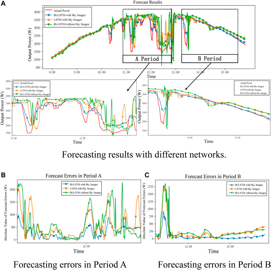
FIGURE 17. Forecasting results and errors with different methods. (A) Forecasting results with different networks. (B) Forecasting errors in Period A (C) Forecasting errors in Period B.

As shown in Figure 17C, the forecast error is small, and all three methods can achieve good results when the weather conditions are sunny. When the weather is cloudy, the output power of PV systems includes large power fluctuations, and the forecast errors of Bi-LSTM with cloud information are much smaller than those of the LSTM with cloud information and Bi-LSTM without cloud information. The detailed indices for the forecasting results are listed in Table 3.

TABLE 3

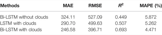
TABLE 3. Evaluation results with different evaluation indices.

The duration of the forecasting time is another important factor affecting the accuracy of the forecasting results. The performance indices with different durations are listed in Table 4.

TABLE 4

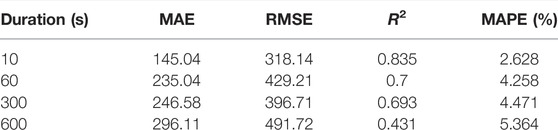
TABLE 4. Evaluation results with different prediction durations.

The number of layers in the LSTM network affects both the training speed and forecast accuracy. The performance of the LSTM network is insufficient when the number of layers is small. However, increasing the number of layers may reduce the generalization capability and increase the training time of the network. The detailed results are shown in Table 5.

TABLE 5

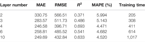
TABLE 5. Results with different number of layers.

The results of the case studies indicate that the proposed data-driven method can predict the output power of a PV system with sufficient accuracy. The effects of clouds on the radiation striking the PV panels can be calculated using the proposed feature of the key area brightness. The Bi-LSTM network can improve accuracy and training efficiency.

Conclusion

This study proposed a data-driven ultra-short PV forecasting method. Several different features were extracted from the sky images photographed in real time. The effects of cloud on the irradiation of the PV panels was evaluated using these features. A Bi-LSTM structure was proposed to consider the cloud features and output power in past time intervals. The proposed Bi-LSTM network was used to determine the average output power during the following 5 min with sufficient accuracy, especially under cloudy weather conditions. The proposed ultra-short PV forecast method can be integrated with optimal operation models and used to dispatch controllable operation resources to maintain the power balance of power systems. Moreover, the sky images are captured from cameras installed at the PV panels. These cameras can be cleaned with the same cycle of the maintenance schedule of the PV stations to avoid the reduced image quality caused by bad weathers. The proposed method is potential to be applied with a PV stations with multiple cameras to obtain the speed of clouds with higher accuracy. Future work will focus on extending the forecasting method to predict the time series of output power in the future.

Data Availability Statement

The original contributions presented in the study are included in the article/Supplementary Material, further inquiries can be directed to the corresponding author.

Author Contributions

LL wrote the draft and proposed the idea XB trained the AI network, built the experiment system, and carried out the case studies.

Funding

This research was funded by National Natural Science Foundation of China, Grant Number 52077045 and in part by the Research Grants Council of the Hong Kong Special Administrative Region, China, under Project T23-701/20-R.

Conflict of Interest

XB was employed by the company Guangzhou Power Supply Bureau of Guangdong Power Grid Corporation.

The remaining authors declare that the research was conducted in the absence of any commercial or financial relationships that could be construed as a potential conflict of interest.

Publisher’s Note

All claims expressed in this article are solely those of the authors and do not necessarily represent those of their affiliated organizations, or those of the publisher, the editors and the reviewers. Any product that may be evaluated in this article, or claim that may be made by its manufacturer, is not guaranteed or endorsed by the publisher.

References

Bay, H., Ess, A., Tuytelaars, T., and Van Gool, L. (2008). Speeded-Up Robust Features (SURF). Comput. Vis. Image Underst. 110 (3), 346–359. doi:10.1016/j.cviu.2007.09.014

CrossRef Full Text | Google Scholar

Cho, K., Merrienboer, B. V., Gülçehre, Ç., Bahdanau, D., Bougares, F., Schwenk, H., et al. (2014). “Learning Phrase Representations Using RNN Encoder Decoder for Statistical Machine Translation,” in Proceedings of the 2014 Conference on Empirical Methods in Natural Language Processing (EMNLP), Doha, Qatar.

CrossRef Full Text | Google Scholar

Farhangi, H. (2010). The Path of the Smart Grid. IEEE Power Energy Mag. 8 (1), 18–28. doi:10.1109/mpe.2009.934876

CrossRef Full Text | Google Scholar

Fu, Y., Chai, H., Zhen, Z., Wang, F., Xu, X., Li, K., et al. (2021). Sky Image Prediction Model Based on Convolutional Auto-Encoder for Minutely Solar PV Power Forecasting. IEEE Trans. Ind. Appl. 57 (4), 3272–3281. doi:10.1109/tia.2021.3072025

CrossRef Full Text | Google Scholar

Gers, F. A., Schmidhuber, J., and Cummins, F. (2000). Learning to Forget: Continual Prediction with LSTM. Neural Comput. 12, 2451–2471. doi:10.1162/089976600300015015

PubMed Abstract | CrossRef Full Text | Google Scholar

Grainger, B. M., Reed, G. F., Sparacino, A. R., and Lewis, P. T. (2014). Power Electronics for Grid-Scale Energy Storage. Proc. IEEE 102 (6), 1000–1013. doi:10.1109/jproc.2014.2319819

CrossRef Full Text | Google Scholar

Greff, K., Srivastava, R. K., Koutnik, J., Steunebrink, B. R., and Schmidhuber, J. (2017). LSTM: A Search Space Odyssey. IEEE Trans. Neural Netw. Learn. Syst. 28 (10), 2222–2232. doi:10.1109/tnnls.2016.2582924

PubMed Abstract | CrossRef Full Text | Google Scholar

Grigorescu, C., Petkov, N., and Westenberg, M. A. (2003). Contour Detection Based on Nonclassical Receptive Field Inhibition. IEEE Trans. Image Process. 12 (7), 729–739. doi:10.1109/tip.2003.814250

PubMed Abstract | CrossRef Full Text | Google Scholar

Hochreiter, S., and Schmidhuber, J. (1997). Long Short-Term Memory. Neural Comput. 9 (8), 1735–1780. doi:10.1162/neco.1997.9.8.1735

PubMed Abstract | CrossRef Full Text | Google Scholar

Huang, A. Q., Crow, M. L., Heydt, G. T., Zheng, J. P., and Dale, S. J. (2011). The Future Renewable Electric Energy Delivery and Management (FREEDM) System: The Energy Internet. Proc. IEEE 99 (1), 133–148. doi:10.1109/jproc.2010.2081330

CrossRef Full Text | Google Scholar

Ipakchi, A., and Albuyeh, F. (2009). Grid of the Future. IEEE Power Energy Mag. 7 (2), 52–62. doi:10.1109/mpe.2008.931384

CrossRef Full Text | Google Scholar

Jiang, L., Chi, Y., Qin, H., Pei, Z., Li, Q., Liu, M., et al. (2011). Wind Energy in China. IEEE Power Energy Mag. 9 (6), 36–46. doi:10.1109/mpe.2011.942350

CrossRef Full Text | Google Scholar

Liang, L., Hou, Y., and Hill, D. J. (2017). Design Guidelines for MPC‐Based Frequency Regulation for Islanded Microgrids with Storage, Voltage, and Ramping Constraints. IET Renew. Power Gener. 11 (8), 1200–1210. doi:10.1049/iet-rpg.2016.0242

CrossRef Full Text | Google Scholar

Liu, J., Fang, W., Zhang, X., and Yang, C. (2015). An Improved Photovoltaic Power Forecasting Model with the Assistance of Aerosol Index Data. IEEE Trans. Sustain. Energy 6 (2), 434–442. doi:10.1109/tste.2014.2381224

CrossRef Full Text | Google Scholar

Muja, M., and Lowe, D. G. (2014). Scalable Nearest Neighbor Algorithms for High Dimensional Data. IEEE Trans. Pattern Anal. Mach. Intell. 36 (11), 2227–2240. doi:10.1109/tpami.2014.2321376

PubMed Abstract | CrossRef Full Text | Google Scholar

Siami-Namini, S., Tavakoli, N., and Namin, A. S. (2019). “The Performance of LSTM and BiLSTM in Forecasting Time Series,” in 2019 IEEE International Conference on Big Data. doi:10.1109/bigdata47090.2019.9005997

CrossRef Full Text | Google Scholar

Wan, C., Zhao, J., Song, Y., Xu, Z., Lin, J., and Hu, Z. (2015). Photovoltaic and Solar Power Forecasting for Smart Grid Energy Management. CSEE Power Energy Syst. 1 (4), 38–46. doi:10.17775/cseejpes.2015.00046

CrossRef Full Text | Google Scholar

Wen, H., Du, Y., Chen, X., Lim, E., Wen, H., Jiang, L., et al. (2021). Deep Learning Based Multistep Solar Forecasting for PV Ramp-Rate Control Using Sky Images. IEEE Trans. Ind. Inf. 17 (2), 1397–1406. doi:10.1109/tii.2020.2987916

CrossRef Full Text | Google Scholar

Yan, J., Hu, L., Zhen, Z., Wang, F., Qiu, G., Li, Y., et al. (2021). Frequency-Domain Decomposition and Deep Learning Based Solar PV Power Ultra-Short-Term Forecasting Model. IEEE Trans. Ind. Appl. 57 (4), 3282–3295. doi:10.1109/tia.2021.3073652

CrossRef Full Text | Google Scholar

Zhang, R., Ma, H., Saha, T. K., and Zhou, X. (2021). Photovoltaic Nowcasting With Bi-Level Spatio-Temporal Analysis Incorporating Sky Images. IEEE Trans. Sustain. Energy 12 (3), 1766–1776. doi:10.1109/tste.2021.3064326

CrossRef Full Text | Google Scholar

Zhang, X., Li, Y., Lu, S., Hamann, H. F., Hodge, B.-M., and Lehman, B. (2019). A Solar Time Based Analog Ensemble Method for Regional Solar Power Forecasting. IEEE Trans. Sustain. Energy 10 (1), 268–279. doi:10.1109/tste.2018.2832634

CrossRef Full Text | Google Scholar

Zhen, Z., Liu, J., Zhang, Z., Wang, F., Chai, H., Yu, Y., et al. (2020). Deep Learning Based Surface Irradiance Mapping Model for Solar PV Power Forecasting Using Sky Image. IEEE Trans. Industry Appl. 56 (4), 3385–3396. doi:10.1109/tia.2020.2984617

CrossRef Full Text | Google Scholar

Zhen, Z., Pang, S., Wang, F., Li, K., Li, Z., Ren, H., et al. (2019). Pattern Classification and PSO Optimal Weights Based Sky Images Cloud Motion Speed Calculation Method for Solar PV Power Forecasting. IEEE Trans. Ind. Appl. 55 (4), 3331–3342. doi:10.1109/tia.2019.2904927

CrossRef Full Text | Google Scholar