Wind Turbine Gearbox Failure Detection Through Cumulative Sum of Multivariate Time Series Data

The wind energy industry is continuously improving their operational and maintenance practice for reducing the levelized costs of energy. Anticipating failures in wind turbines enables early warnings and timely intervention, so that the costly corrective maintenance can be prevented to the largest extent possible. It also avoids production loss owing to prolonged unavailability. One critical element allowing early warning is the ability to accumulate small-magnitude symptoms resulting from the gradual degradation of wind turbine systems. Inspired by the cumulative sum control chart method, this study reports the development of a wind turbine failure detection method with such early warning capability. Specifically, the following key questions are addressed: what fault signals to accumulate, how long to accumulate, what offset to use, and how to set the alarm-triggering control limit. We apply the proposed approach to 2 years’ worth of Supervisory Control and Data Acquisition data recorded from five wind turbines. We focus our analysis on gearbox failure detection, in which the proposed approach demonstrates its ability to anticipate failure events with a good lead time.

Introduction

Wind energy is among the fastest-growing renewable energy sources. The year of 2020 has been marked as the biggest year ever with a record 93 GW of new installation (GWEC, 2021). IEA (2020) predicted that over 2023-25, average annual wind energy additions could range from 65 to 90 GW. Adding to the growth, it was also reported that wind energy has become more cost competitive as indicated by a decreasing trend of the levelized cost of energy (LCOE) (IEA, 2020; U.S. Department of Energy, 2021; GWEC, 2021). A significant portion of LCOE is related to turbine performance (availability and production) and reliability; for instance, Dao et al. (2019) reported a strong and nonlinear relationship between wind turbine reliability and operations and maintenance (O&M) cost. The better the reliability and performance, the lower the LCOE. The challenge is how to keep the O&M cost low while maintaining a desired level of performance and reliability.

Detecting a component failure relies on identifying anomalies or specific patterns in a dataset. The most commonly used data inputs for anomaly detection in wind turbines are those from the Supervisory Control and Data Acquisition (SCADA) system (Leite et al., 2018), failure logs, vibration (Natili et al., 2021; Pang et al., 2021), and occasionally particle counts, status logs, andmaintenance records. Chapter 12 of Ding (2019) explains the two major schools of thought of fault diagnosis and anomaly detection: a statistical learning-based approach (Orozco et al., 2018; Vidal et al., 2018; Ahmed et al., 2019; Moghaddass and Sheng, 2019; Ahmed et al., 2021b; Ahmed et al., 2021; Xiao et al., 2022), including control chart approaches (Hsu et al., 2020; Riaz et al., 2020), and physical model-based approach (Guo and Keller, 2020). There are naturally approaches combining the two schools of thought (Yampikulsakul et al., 2014; Guo et al., 2020; Hsu et al., 2020; Yucesan and Viana, 2021). In this study, we focus on the statistical learning-based approaches.

Depending on the availability of data labels in a training set, statistical learning-based approaches can be categorized as supervised and unsupervised learning. Supervised learning needs appropriately labeled data to train a predictive model, which, once a future input is given, predicts whether the future instance is a fault/failure event. Least-squares support vector regression (LS-SVR) (Yampikulsakul et al., 2014), support vector machine or regression (Vidal et al., 2018; Natili et al., 2021), random forest (Hsu et al., 2020; Pang et al., 2021), XG-Boost and long short-term memory (LSTM) networks (Desai et al., 2020; Xiao et al., 2022) are examples of this category. Labeling the training data can be challenging because the fault tags are often added manually. Labeling the training data can also be tricky. Usually, the data point corresponding to the failure instance is labeled as a failure and all else are labeled as normal. Consider the typical SCADA data that are recorded every 10 min. What such labeling means is that one of the 10-min data point is labeled as faulty or a failure, and the data points even only 10 min before and after being labeled as normal. But is this a good labeling practice? Since the failures are relatively rare, what such labeling generates is highly imbalanced data, causing many off-the-shelf statistical learning methods to render weak detection (Byon et al., 2010; Pourhabib et al., 2015). If more data points than those at the failure instance are to be labeled, then the questions of how many and which data points should be labeled arise but are hard to address. Some work (Desai et al., 2020; Williams et al., 2020) choose to label additional data points prior to the failure instance—so far such action remains ad hoc.

When the data label is not available, unsupervised learning is the appropriate approach for anomaly detection. Unsupervised learning relies on the structure or pattern of the dataset to separate any anomalies from the normal data (Wang et al., 2012). One recent developed approach is based on the minimum spanning tree-based distance (Ahmed et al., 2019; Ahmed et al., 2021b; Ahmed et al., 2021), which works based on the connectedness of data points with their neighbor and identifies anomalies that are sufficiently different from the majority of its neighbors. Ahmed et al. (2019) demonstrated the application of such an unsupervised learning approach for anomaly detection in hydropower turbines.

In a real-world problem, there is another category approach, referred to as one-class classification (Park et al., 2010) or semi-supervised learning, or in other words, in between the supervised and unsupervised approach. The one-class classification uses only the data under normal operating conditions. This could be because for a turbine, no failure has been recorded yet, or a small number of failures were recorded but the analysts felt they would be better off not using the failure event data. In this case, one can train a model on the normal data and test whether a future observation conforms with the established normalcy. If not, then such an observation is classified as an anomaly. Yampikulsakul et al. (2014) offers one such approach, as they used the residuals from the modeled normal data to determine abnormality. Technically, the control chart-based methods (Hsu et al., 2020; Riaz et al., 2020; Xu et al., 2020; Dao, 2021; Dao, 2022) fall into this category.

Despite the advancement in statistical learning and fault detection, most of the fault detection methods mentioned earlier do not accumulate small-magnitude early symptoms effectively over time for symptom tracking. As stated earlier, the current approaches respond to a given event individually, classifying it - as faulty or non-faulty; such approaches are known as point-wise detection. The lack of symptoms accumulation and tracking explains why the current fault detection systems have very limited early warning capability.

Motivated by the desired capability for symptom accumulation and tracking, we noticed one quality-control method, known as the cumulative sum (CUSUM) method (Page, 1954; Page, 1961). CUSUM is a memory-type control chart and particularly noted for its ability to accumulate consecutive sample points in a process over time and thus effectively detect a small shift in the process that memoryless methods would otherwise fall short of detecting.

Even though CUSUM is a well established approach, it is not easy to apply it to turbine failure detection. The implementation on the complex turbine SCADA data would require some major modification. For this purpose, Dao (2021) adapted a CUSUM-based approach that were typically used to test structural changes in economic and financial time series data. The approach cumulated the standardized residuals after the generator speed is fit through a linear mode and then used the residuals to establish the monitoring chart, of which the control limits were approximated as a function of the data size. This CUSUM-based approach was reported to detect two known failures just a few minutes before the failures took place. Xu et al. (2020) designed an adaptive CUSUM chart to monitor the residuals after the bearing temperature is fit through a random forest model. The alarms from the adaptive CUSUM were issued daily instead of every 10 min to reduce the alarm frequency, but there was not reporting that how early the failures could be detected.

Similarly inspired by the concept and method of CUSUM, we set out to develop a symptom-accumulating method for fault detection with early warning capability. We targeted weeks ahead detection rather than minutes or hours ahead. But the plain CUSUM (also referred to as the vanilla version of CUSUM) is not effective in handling the complexities associated with a wind turbine system. The new method needs to address the four specific questions:

• Which fault signals to accumulate? The plain CUSUM accumulates the raw measurements, or its sample average. Our research shows that for the turbine SCADA data in a high-dimensional space, accumulating the raw measurements or its sample average is not effective.

• The use of an offset. What is actually accumulated is the difference between the anomaly score and an offset value, rather than the anomaly score itself. The offset value is used to prevent the accumulation of background noises. This is the aspect that the new method remains the same as the plain CUSUM method, but the way to choose the offset will be different.

• How long to accumulate? In the plain CUSUM method, the accumulation is allowed until the instance of failure events. Should we do the same for turbine fault detection, it will cause too many false positives. We therefore set an accumulation window size to balance the two types of error in detection (i.e., false positives versus false negatives).

• Setting the control limit. The control limit is also known as the decision threshold. In the plain CUSUM method, the control limit is chosen for producing the desirable average run length performance metric. In our design, we need to link the decision outcomes with the monetary gains and losses associated with the detection performance metrics, specifically, the true positives, false positives, and false negatives.

To demonstrate and evaluate the proposed approach, we implement the approach on real wind turbine datasets with a focus on gearbox failures. It is not surprising that the gearbox is chosen for the demonstration purpose as it is the most popular component to investigate (Guo et al., 2020; Guo and Keller, 2020; Mauricio et al., 2020; Liu et al., 2021). Not only has it been one of the components that contribute most to turbine downtime (Pinar Pérez et al., 2013; Tchakoua et al., 2014; Pfaffel et al., 2017; Dao et al., 2019; Liu et al., 2021), but the replacement cost is also prohibitively high (Liu et al., 2021).

The rest of the article is organized as follows. Introduction explains the dataset used in this study. Introduction provides details about the proposed method, i.e., the answer to the aforementioned four questions. Introduction presents the implementation, results, interpretations, and analysis concerning the proposed method. Finally, Introduction summarizes this work.

Data

The data we use in this work are retrieved from an online open data source (EDP, 2018b). An account registration is required but such registration is free. Except for the dataset about the geographical location of the turbines, all of the datasets from the open data source, including all that we used, are granted a free use CC-BY-SA license.

The open source provides SCADA datasets of five wind turbines from the same wind farm with a 2-years time span, which include: a set of signals recorded from the wind turbines, a set of meteorological tower data, a failures log, and a status log. The datasets were collected from January 2016 through December 2017. All these files are provided with the Wind Farm one tag on the file names. They are split into 2016 and 2017 data. The five wind turbines in the data are named as T01, T06, T07, T09, and T11. All turbines belong to the same model in a 2-MW class with a three-stage planetary/spur gearbox. The cut-in, rated, and cut-out wind speeds are 4 m/s, 12 m/s, and 25 m/s, respectively.

We mainly use signals from wind turbines and the failures log for the analysis. These data are of good quality, as there are only a few missing values. The 2-years recorded signals from five turbines are stored in. csv files, forming a table that comprises 521,784 rows and 83 columns when combined together.

The rows are the time series. With a 10-min time resolution, the number of data points per turbine per year is 52,560 without any missing values. For five turbines and 2 years, the total data amount would ideally be 525,600. The actual records of 521,784 account for slightly over 99% of the ideal total data.

The 83 columns include the turbine ID, the time stamp, and 81 environmental (outside the nacelle) and turbine condition (inside the nacelle) variables. The environmental variables include wind speed, ambient temperature, wind direction, among others, whereas the condition variables include turbine component temperature, speed of the rotating components, active power, etc. The 81 variables are not all physically distinct. Some are associated with the same physical attribute but provides different statistics, such as the average, minimum, maximum and standard deviation of wind speed in the 10-min periods.

Among the 521,784 records over 2 years, there are a total of 28 failures recorded in the log file. The source of failures varies but it can be grouped based on the components, i.e., generator, generator bearing, gearbox, transformer, and hydraulic group.

We focus our analysis on the gearbox failure detection. For this purpose, we split the data into 80:20 of training set and testing set. This means the first 20 months of data are used for training and the four last months are used for test. In other words, the training data covers from 1 January 2016 through 31 August 2017 and the test data covers from 1 September 2017 through 31 December 2017. Four gearbox failures were recorded for the entire 2-years period, two are in the training set and the rest are in the test set. Table 1 lists the gearbox failures information.

TABLE 1

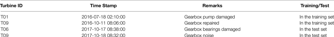
TABLE 1. Gearbox failure log.

The datasets were previously given as part of two open challenges: The EDP Wind Turbine Failure Detection Challenge 2021 and Hack the Wind 2018. The turbine signals data were very clean and well organized. As part of the 2021 Challenge, we were supposed to take the data as is. Only some basic data cleaning were performed such as removing all the missing values and checking whether data values are within reasonable physical ranges. No other information was provided to us (e.g., how the data provider pre-processed their data is unknown). We did downsize the data resolution from 10-min to 1-h averages and normalize the data prior to the implementation of our proposed method.

Methods

Let us first quickly recap how CUSUM works, which offers the blueprint for the design of our proposed method.

Consider a CUSUM control chart for detecting a change in process mean. Denote by μ₀ the baseline mean. The input signal is the sample observation, denoted by x_t at time t. At any given time, a small sample of multiple x_t’s, say five of them, are observed. Then the sample average, ${\bar{x}}_t$, is computed and used as the input value to a CUSUM chart. The sample size is denoted by n. When n = 1, i.e., at any given time, a single observation is made, then the sample average is the same as the original observation, i.e., ${\bar{x}}_t=x_t$. This n = 1 circumstance represents the majority of the cases when CUSUM is applied. Taking x_t, the CUSUM method computes a score, through the CUSUM formula,

$C_t=\max \left\{0,C_{t-1}+\left[x_t-{\mu }_0-K\right]\right\},(1)$

where K is the offset, and the initial condition, C₀, is set to zero. The standard CUSUM separates the upward change from the downward change and thus put a superscript “+” on the above CUSUM score, i.e., $C_t^{+}$, and create a slightly modified formula for $C_t^{-}$ for downward detection.

Apparently, the CUSUM score, C_t, accumulates the difference of x_t − μ₀ and K, where x_t − μ₀ is the fluctuation of the process around its baseline mean. To detect, a control limit H is imposed. The score, C_t, is compared with H, and an alarm is triggered when C_t exceeds H. The two parameters, H and K, are the so-called design parameters of a CUSUM method, which are chosen using the training data. The training data are considered all in control, so that the CUSUM method falls in the category of one-class classification or semi-supervised learning.

Our CUSUM-inspired method follows the same procedure, but we need to provide our unique and specific solutions to the four questions raised in Methods. Figure 1 illustrates the overall flow.

FIGURE 1

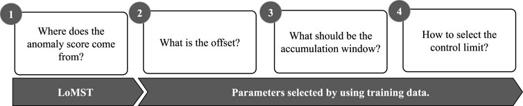
FIGURE 1. The flowchart of the main steps in the CUSUM-inspired detection method.

1. What is used as the anomaly score?

Denote the turbine data matrix as X_m×p≔{x_tj} where t = 1, … , m, j = 1, … , p, and for the whole dataset m = 521, 784 and p = 83. For the training data, its m is about 80% of the whole dataset. At any time point, we have a single observation of dimension p, denoted by ${\mathit{x}}_t≔{(x_{t1},x_{t2},\dots ,x_{tp})}^T$.

This x_t cannot be directly plugged into Eq 1, because Eq 1 is for a univariate detection, meaning that the x therein is of dimension p = 1. We acknowledge the existence of multivariate CUSUM, which is of the same concept and uses a similar formula as the univariate CUSUM but can take in a multivariate input, i.e., a vector of x_t.

Using a multivariate CUSUM does not produce good detection outcomes for turbine failure detection. When we looked into the reasons behind, we think that one previous research provided the explanation. Ahmed et al. (2019) argued that in a multidimensional data space, anomaly and fault detection should not use Euclidean distances to differentiate data instances, because there is a high likelihood that the multidimensional data space embeds a manifold, known as the manifold hypothesis (Fefferman et al., 2016). In fact, the existence of manifold is rather ubiquitous and confirmed in many applications since its discovery in computer vision (Tenenbaum et al., 2000). A manifold is an inherent data structure restricting the reachability of data instances between each other. When such manifold embedding happens, the use of Euclidean distance is no longer appropriate and could mislead a detection system. Methods of Ding (2019) presents a detailed account of various distance metrics used in differentiating data instances in statistical machine learning. Methods specifically presents an illustration of how Euclidean distance mis-characterizes the similarity between data instances, thereby leading to wrong detection.

In the multivariate CUSUM, the distance matric used is the statistical distance (explained in detail in Methods in Ding (2019)), which is a variant of Euclidean distance. For multidimensional data space embedding manifold, using the statistical distance suffers the same problem as using the Euclidean distance.

The solution for addressing this problem is to use a geodesic distance. But the geodesic distance is not always directly computable but can often be approximated by some other means. Ahmed et al. (2019) propose to use the minimum spanning tree (MST) to approximate the geodesic distance. They argued that using MST provides one of the best approximations because of two good properties of MST—minimum ensures the tightest distance and spanning implies ergodicity. They demonstrate, using 20 benchmark datasets and comparing them with 13 existing methods, a clear advantage of using the MST-based anomaly detection method.

Therefore, we choose to adopt the MST approach for our anomaly score calculation. The detailed procedure is explained in Methods of Ding (2019), so we will not repeat it here. Also, Ahmed et al. (2019) makes their computer code available (Ahmed et al., 2021a), which facilitates the implementation of the MST-based anomaly score computing algorithm. The computer code includes the construction of the MST on a given dataset, so that users do not need to construct the MST by themselves, either.

If we treat the MST-based anomaly score computing procedure as a black box, the input to the black box is the multivariate vector x_t and the output of the box is a univariate anomaly score. Note that using the EDP data for computing the anomaly score, we use the combined data from all five turbines together. Let us denote the anomaly score by z_t, which is normalized to take a value between 0 and 1. A greater score implies a higher possibility for a data point to be anomalous. There are a few variants of the MST-based anomaly score due to the continuous development on this topic (Ahmed et al., 2021b; Ahmed et al., 2021). The specific variant we used for turbine fault detection is the Local MST (LoMST) originally proposed by Ahmed et al. (2019) and again exhibited in Chapter 12 of Ding (2019).

2. How long to accumulate and set the offset?

Here we discuss the second and third questions together.

Like all point-wise detection methods reviewed in Section 1, the MST-based methods and its variants (Ahmed et al., 2019; Ahmed et al., 2021b; Ahmed et al., 2021) do not do symptom accumulation. For this reason, it does not include an offset. The concept of accumulation window does not apply, either.

As shown in Eq 1, the offset, K, is explicitly included in CUSUM. On the other hand, CUSUM does not explicitly impose an accumulation window size. CUSUM is designed to detect simple changes like a mean shift. It is the fluctuation around the mean, x_t − μ₀, less the offset K, that gets accumulated. This value can be positive or negative. When x_t − μ₀ − K is negative for multiple steps, it could turn C_t to zero, which is known as a reset. With this reset mechanism, CUSUM allows its score to continuously accumulate without manually setting the accumulation window size. The duration when C_t is non-negative can be naturally considered as the de facto accumulation window.

The wind turbine failure detection is far more complicated than a mean shift detection. It is challenging to know around which baseline its anomaly score z_t fluctuates. This means that its counterpart of μ₀ is difficult to decide. What we propose to do is to take a direct difference between z_t and K, i.e., z_t − K. But because K, as an offset, is usually smaller than z_t, z_t − K tends to be positive and does not create the reset mechanism as in CUSUM. If we let z_t − K continue accumulating, the accumulation will almost always exceed the control limit, once given sufficient time, leading to too many false positives. Because of this, for our detection method, we impose an explicit accumulation window size, denoted by W, so that the accumulation resets when reaching to the limit of the accumulation window.

We propose to choose the offset K based on the probability distribution of the anomaly scores. The basic idea is as follows. In the absence of anomalous events, one anticipates a natural fluctuation in the anomaly scores, more or less like a normal distribution. When the actual anomaly score distribution exhibits a long tail going beyond the natural fluctuation, the anomaly scores corresponding to the long tail are deemed truly anomalous, whereas the normal distribution-like portion, symmetric with respect to the average, is considered to correspond to the background noise. Figure 2 illustrates the idea. The vertical dashed line is the chosen offset, which separates the density curve into two parts—the blue part is for the background noises and the red part is for anomalies. The offset is chosen, so that the blue density curve is roughly symmetric and the curve beyond that point becomes almost flat. This selection approach needs visual judgement, so it does entail a certain degree of subjectivity. In this regards, it bears resemblance to the scree plot, which is used to select the number of principal components in a principal component analysis (PCA) (Jolliffe, 2002). The scree plot is also a graph plot based tool that needs a visual judgement to decide on the particular value to choose. Despite such subjectivity, it is still nonetheless the most widely used tool for deciding the number of principal components.

FIGURE 2

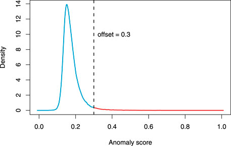
FIGURE 2. The density curve of the anomaly scores of the entire data points. The vertical dashed line marks the offset, which is 0.3 for this particular analysis.

The accumulation window size W will be chosen by making use of the training data. A number of considerations include how many clusters are produced, how distinguishable the clusters are based on the distance between them, and how many clusters actually predict the true failures in the training data. True positives way ahead of a failure event is most desirable. In practice, a certain number of false positives may be tolerated in exchange for detecting the true failure events over the cases of few false positives but many missed detections, because the cost of a missed detection exceeds by a large margin that of a false positive. The specific trade-off between these cost components is to be optimized using a cost/savings utility function, to be discussed in the sequel.

3. How to set the control limit?

To determine the control limit, we make use of the information from the failure log to tag the failure time and then use the training data to optimize the control limit. Different from the plain CUSUM chart that optimizes their average run length performance, we adopt a utility function that connects the failure detection performance with monetary gains and losses. The basic idea is to choose a control limit that maximizes the true detection, while at the same time regulating the number of false positives at an acceptable level. A utility function is an objective function that unifies the gains and losses from different actions. The specific utility function is adopted from an open challenge—Hack the Wind 2018 (EDP, 2018a)—for its practical relevance and realistic monetary parameters (as it is set by a major wind company). We believe the function adopted bears general applicability, although the specific monetary parameters may be adjusted for particular owners/operators and applications.

Three detection possibilities are considered: true positives (TP), false positives (FP), and false negatives (FN). When a true detection happens, a potential saving is in order. The saving amount is related to how early such warning can be issued. Therefore, the TP saving is set in the Hack the Wind 2018 challenge as

$T{P}_{saving}=\sum _{i=1,\dots ,\#\text{TP}}\left(R_{cost}-M_{cost}\right)\left(\frac{\mathrm{\Delta }{t}_i}{60}\right),(2)$

where #TP is the number of true positives, R_cost and M_cost are the replacement and maintenance costs (also known as repair cost), respectively, and Δt_i is the number of days ahead of the failure time. The savings function in Eq 2 assumes that 60 days before the failure event is where the maximum savings can be achieved. The savings decreases as the detection happens closer to the instance of the failure.

When a false negative happens, it means a miss detection. Then, the cost is the replacement cost, which is the most costly option. When a false detection happens, the consequence is an inspection cost, denoted by I_cost. As such, the FN and FP cost components are, respectively,

$\begin{array}{cc}\hfill F{N}_{cost}& =\#\text{FN}\times R_{cost},\hfill \\ \hfill F{P}_{cost}& =\#\text{FP}\times I_{cost},\hfill \end{array}(3)$

where #FN and #FP are the number of the false negatives and false positives, respectively. The utility function, U(H), combines all the savings and cost elements, where H is the control limit. The control limit is decided by maximizing the utility function, i.e.,

$\begin{array}{cc}\hfill & \underset{H}{\max }U\left(H\right),\hfill \\ \hfill & \text{where}U\left(H\right)=T{P}_{saving}-F{N}_{cost}-F{P}_{cost}.\hfill \end{array}(4)$

In the Hack the Wind 2018 challenge, the early warning is assumed up to 60 days in advance. In our study, we extend it to 90 days in advance. This extension is mainly because the source of failures in a wind turbine gearbox varies, from one that is temporary and random to a wear-out failure due to a longtime running in poor working conditions (Liu et al., 2021). The extension is expected to capture this wear-out type of failure. When a failure is not detected before the event, it is considered to be a false negative. When an alarm is issued but with no corresponding failure in the dataset, it is considered to be an FP. In the Hack the Wind 2018 challenge, a detection within 2 days of the failure event is also considered a miss detection, or an FN, as it is too close to the failure event to prevent the failure from happening. We keep the same treatment in this study.

Additional Remarks

As a summary, our CUSUM-inspired failure detection method entails the following main steps:

1) Compute the anomaly scores for all data points of interest; both training and test sets.

2) Subtract the offset value from the raw anomaly scores, so as to flag only those data points with high anomaly scores as anomalies.

3) Use the training data to determine the accumulation window, a maximum time between two consecutive anomaly data points of which the anomaly scores are to be accumulated.

4) Again use the training data to optimize for the control limit H, beyond which the accumulated anomaly score triggers an alarm.

Figure 3 illustrates the step-by-step process of our proposed method when it is applied to the data of T09. In the actual analysis reported in the next section, we use the data pooled from all five turbines, but the concept and method remain the same.

FIGURE 3

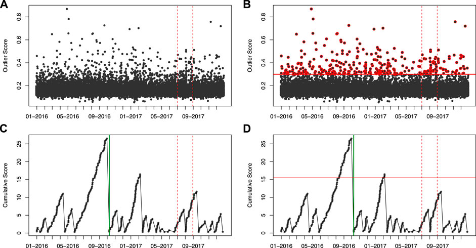
FIGURE 3. Illustration of the actions in the proposed method. In this example, only T09 data is used. In each of the figures, there are two vertical dashed red lines. The one to the right is the time boundary between the training and test data. The one to the left is the 60-days mark before the test set. (A) plots the output of LoMST anomaly score calculation. (B) adds the offset, so that only anomaly scores above the offset are accumulated in the next step. Those scores are highlighted in red color. (C) is the plot of cumulative anomaly score, where one can see the effect of accumulation and tracking. The vertical green line indicates the time of a true gearbox failure recorded in the training data. (D) adds the control limit for detection, which is the horizonal red line. With this control limit, it flags two alarms in the training data and none in the test data. One of the two alarms is a true positive, with the early warning lead time of 89 days and the other is a false alarm.

Results and Discussion

We implement our proposed method aiming at detecting gearbox failures in wind turbines. In this section, we start off explaining further implementation details and the parameters chosen in the proposed detection method. After that, we will discuss the results and evaluate the performance of the method.

Implementation Details and Parameters

Prior to the implementation of the proposed method, we perform data preprocessing and variables selection. The data is originally a 521,784 × 83 matrix. We downsize the number of rows by aggregating data from their original 10-min temporal resolution to 1-h averages. This preprocessing reduces the number of rows to 87,052 for all five turbines, or about 17,400 rows per turbine.

Variables selection is important for screening the available variables into a smaller set of meaningful and highly relevant variables. We conducted various tests to reduce variables that have a high collinearity with other variables. In the end, we select a subset that consists of gearbox oil temperature, gearbox bearing temperature, nacelle temperature, rotor speed, ambient wind direction, and active power. We perform our detection method, as explained in Implementation Details and Parameters, on the data with this subset of variables.

The LoMST anomaly score is computed using the code provided by Ahmed et al. (2021a). In producing the LoMST scores, a local neighborhood size is needed; for that we use 25, which is an empirical choice. The rest of the parameters used in the detection method are: 1) the offset K = 0.3 2) the accumulation window size, W = 7 days, and 3) the control limit, H = 8. In deciding H, the following cost parameters are used in the utility function: R_cost = €100,000, M_cost = €20,000, and I_cost = €5,000. These cost parameters are taken from the Hack the Wind 2018 challenge (EDP, 2018a).

Results

Figure 4 presents the results from the implemented method on the dataset. Recall that there are four gearbox failures recorded within the 2-years time span—two are in the training set and the other two are in the test set. All four failures can be detected by the proposed method.

FIGURE 4

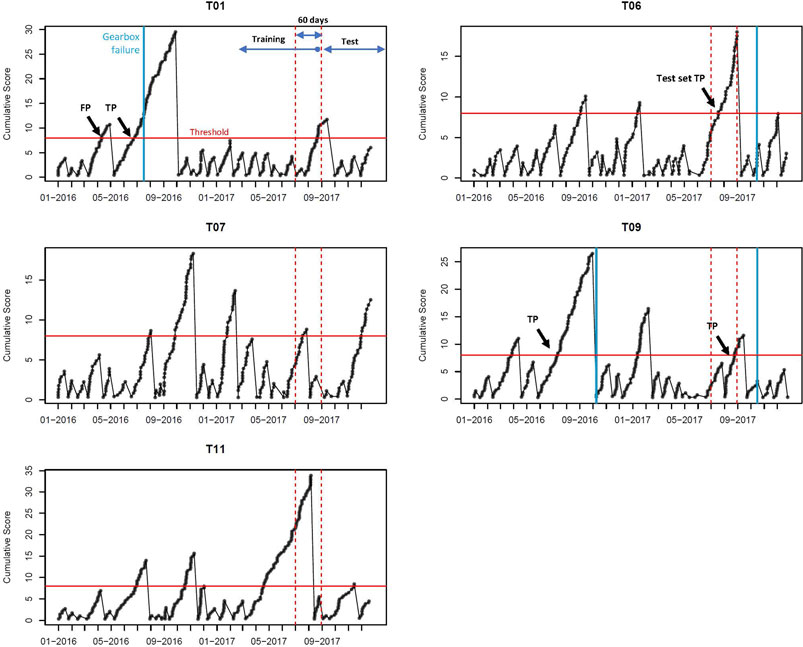
FIGURE 4. Gearbox failure detection results using the proposed method. These results are obtained by setting the control limit as H =8, which is common for all turbines.

Table 2 presents the time of alarm of the gearbox failures based on the results in Figure 4. The early-warning lead time, measured by the alarm-to-failure time, ranges from 21 to 89 days. The average warning lead time based on the training set is 55 days. We also took a close look at the nature of the gearbox failures. Recall that Liu et al. (2021) classified the faults in the wind turbine gearbox into two categories: the wear-out failures and temporary random faults. Note further, from Table 2, that the first and fourth failures are caused by gearbox pump and noise, the second failure’s source is not known, and the third is from the gearbox bearing. A bearing failure is typically a wear-out type that builds up slowly. Our method successfully anticipates this failure, with 89-days lead time. The second failure is most likely of the similar type, but we do not have adequate information, based on the failure remark in the dataset, to be assertive one way or the other. The other two failures—the pump and the noise—are closer to temporary random faults. The lead times of detection are shorter than 60 days.

TABLE 2

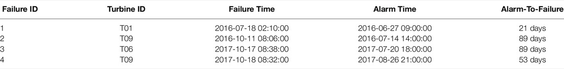
TABLE 2. Gearbox failure detection results summary.

Method Evaluation

Our proposed method works well in anticipating gearbox failures on the given data. Since the method does produce both false positives, in addition to the true detection, we should evaluate the final performance of the method using the total savings formula in Eq 4.

Table 3 presents the savings calculations, as a result of detection performance metrics. We present two scenarios: one uses a common control limit and the other uses individual control limits for each turbine. Following the approach that decides the common control limit for all turbines, the turbinewise control limit could be decided as: 8, 10.5, 18.8, 15.5, and 22 for T01, T06, T07, T09, and T11, respectively. Recall that the common control limit is 8. It turns out that the common control limit works better. It does not have any miss detection, i.e., #FN = 0. As a result, the expected savings for the test data is a positive €130K. By comparison, using the turbinewise control limits would miss one true gearbox failure in the test data and would therefore result in a negative €25K test case savings, or equivalent, a €25K expense for the test cases.

TABLE 3

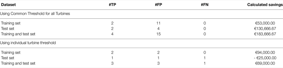
TABLE 3. Calculated savings from detection.

The analysis presented in Table 3 also reaffirms an important message we articulated earlier, which is that detecting a true failure is far more beneficial than reducing a few additional false positives. If we look at the number of false positives (column #FP) in Table 3, we can see that using the turbinewise control limits is very good at reducing the number of false alarms. Yet, the one missing detection costs much more than reducing three false positives in the test data. This is expected, as the replacement cost, the consequence of a missed detection, is twenty times of the inspection cost, the consequence of a false positive. This cost imbalance is generally true, although the specific numerical ratio depends on applications.

To evaluate the merit of the proposed CUSUM-LoMST method, we compare it with the following alternatives:

• Pointwise LoMST. This is the original LoMST method without accumulation.

• Traditional CUSUM, based on (Dao, 2021). This is the CUSUM without using the LoMST score and other modifications made in this paper.

• Correlation-based feature selection, before applying the proposed CUSUM-LoMST method.

• PCA-based feature selection, before applying the proposed CUSUM-LoMST method.

The third and fourth alternatives in the above list are suggested by one of the reviewers for testing whether different feature selection approaches could help improve the performance of the proposed CUSUM-LoMST method. The correlation-based feature selection is based on (Castellani et al., 2021), which is to include the features that have a high Pearson correlation score with the gearbox speed and gearbox bearing temperature. The PCA-based feature selection is to use the first few significant principal components of the features selected by using the Pearson correlation score.

Table 4 presents the failure detection results and the respective savings. From the results we can see that the two alternative feature selection approaches do not help in this case. Their main shortcoming is that they produce more false alarms as compared to the proposed approach. On a positive note, both feature selection approaches still yield positive savings on the test data, as they are able to detect the two true failures.

TABLE 4

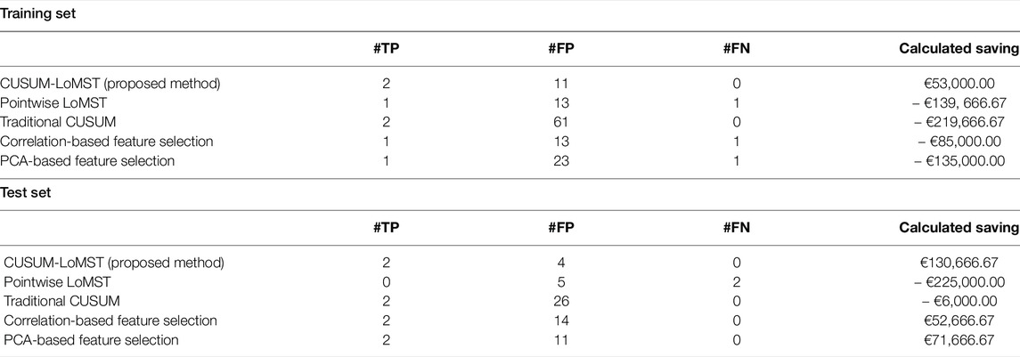
TABLE 4. Comparison of four alternative methods with the proposed CUSUM-LoMST.

The pointwise LoMST and the tradition CUSUM method do not perform well. The principal problem of the pointwise LoMST is its inability to detect the true failures on the test data. This is not surprising, as from the get-go, our argument is that the pointwise methods would miss the failure events without accumulating the signals. The traditional CUSUM method (Dao, 2021) was able to successfully detect the true failures in the test data but did so at the expense of producing a lot more false alarms. In fact, traditional CUSUM produced more false alarms than all other alternatives in comparison. Figure 5 presents a small section (the last quarter of Year 1) of the CUSUM plot. We notice that the plot suffers from seasonal effect and it has to be reset several times; otherwise the CUSUM score will stay outside the control limits for very long time. The high number of false alarms eventually forces the traditional CUSUM method to enter the region of economic loss (or negative savings) on the test data.

FIGURE 5

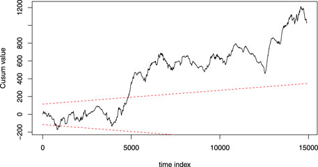
FIGURE 5. An example of CUSUM plot based on the method in (Dao, 2021). The time axis is in the unit of 10 min, as the method in (Dao, 2021) uses 10-min data. This plot covers the first quarter (3 months) of the data. In this particular set of data, the plot goes outside the control limit twice; once went out of the lower limit and once of the upper limit. After going up beyond the upper limit at around 5000^th data point, the plot almost consistently stays above the line.

Conclusion

We propose a method that combines the use of LoMST and a CUSUM approach for detecting anomalies and failures. This method is applied to 2 years’ worth of wind turbine data for detecting gearbox failures in wind turbines. Compared to pointwise detection methods without accumulation or a traditional CUSUM method without adaptation to the wind turbine specifics, the proposed CUSUM-LoMST method produces better detection outcomes and longer lead time, leading to more savings to the industry.

Through this study, we would like to offer the following insights:

• Correctly detecting true failure events with sufficient lead time is far more important than keeping the number of false alarms low. This is not to say that reducing false alarms is not important. But a detection method that does not detect is practically useless. Until the day when one reaches the ideal state of having both high detection rates and low false positive rates, the emphasis should be prioritized towards detection capability.

• Accumulating small-magnitude symptoms is key to enable early-warning capability. But the very action of accumulation exacerbates the delicate trade-off between true detections, false positives, and false negatives, which means that accumulation-capable methods need a careful design to strike the right balance.

• For the detection in a multidimensional space, selecting the right variables and reducing them further into a scalar anomaly score for accumulation is a challenging job, but the final detection performance depends heavily on such choices. Our proposed use of the MST-based anomaly scores appears advantageous, at least for the data we tested. But we acknowledge that on this aspect much more research is needed to make the treatment systematic and less subjective.

We did apply the proposed CUSUM-LoMST detection method to other faults in the EDP Open Data, which includes those from transformer, generator, generator bearing, and hydraulic groups. In those detections, our proposed method remains strong in terms of detection power, but the number of false alarms increases too fast, overwhelming the benefit of the detections and sometimes tipping the balance over toward an overall loss. Continuing the improvement so that the right balance of true detections and false alarms can be reached is indeed our ongoing research pursuit.

Data Availability Statement

Publicly available datasets were analyzed in this study. The datasets analyzed for this study can be found in the Open EDP website https://opendata.edp.com/explore/?refine.keyword=visible&sort=modified.

Author Contributions

EL, SS, and YD contribute to the formulation of the problem. EL and YD contribute to the design of the solution method. EL contributes to the implementation and fine-tuning of the method, while SS and YD provide technical advices. EL and YD contribute to the writing of the paper and SS contribute to the editing and comment of the paper.

Funding

Latiffianti’s research is supported by a Fulbright Scholarship in collaboration with the Indonesian Government (DIKTI-Funded Fulbright). Ding’s research is partially supported by NSF grants IIS-17411731 and CCF-1934904. This work was authored (in part) by the National Renewable Energy Laboratory, operated by Alliance for Sustainable Energy, LLC, under Contract No. DE-AC36-08GO28308 for the U.S. Department of Energy. Funding provided by the U.S. Department of Energy Office of Energy Efficiency and Renewable Energy Wind Energy Technologies Office.

Author Disclaimer

The views expressed in the article do not necessarily represent the views of the DOE or the U.S. Government. The U. S. Government retains and the publisher, by accepting the article for publication, acknowledges that the U. S. Government retains a nonexclusive, paid-up, irrevocable, worldwide license to publish or reproduce the published form of this work, or allow others to do so, for U. S. Government purposes.

Conflict of Interest

The authors declare that the research was conducted in the absence of any commercial or financial relationships that could be construed as a potential conflict of interest.

Publisher’s Note

All claims expressed in this article are solely those of the authors and do not necessarily represent those of their affiliated organizations, or those of the publisher, the editors and the reviewers. Any product that may be evaluated in this article, or claim that may be made by its manufacturer, is not guaranteed or endorsed by the publisher.

Acknowledgments

The authors acknowledge Dr. Sarah Barber, Wind Energy lead at the Eastern Switzerland University of Applied Sciences and President of the Swiss Wind Energy R&D Network, and her WeDoWind platform for hosting a 2021 Data Challenge using the EDP Open Data. The solution method was conceived when the first author participated in the 2021 Data Challenge under the supervision of the two senior authors.

References

Ahmed, I., Dagnino, A., and Ding, Y. (2019). Unsupervised Anomaly Detection Based on Minimum Spanning Tree Approximated Distance Measures and its Application to Hydropower Turbines. IEEE Trans. Autom. Sci. Eng. 16, 654–667. doi:10.1109/tase.2018.2848198

CrossRef Full Text | Google Scholar

Ahmed, I., Dagnino, A., and Ding, Y. (2021a). Dataset and Code for “Unsupervised Anomaly Detection Based on Minimum Spanning Tree Approximated Distance Measures and its Application to Hydropower Turbines”. [Dataset]. Zenodo Data Sharing Platform. doi:10.5281/zenodo.5525295

CrossRef Full Text | Google Scholar

Ahmed, I., Hu, X. B., Acharya, M. P., and Ding, Y. (2021b). Neighborhood Structure Assisted Non-negative Matrix Factorization and its Application in Unsupervised Point-wise Anomaly Detection. J. Mach. Learn. Res. 22 (34), 1–32.

Google Scholar

Ahmed, I., Galoppo, T., Hu, X., and Ding, Y. (2021). Graph Regularized Autoencoder and its Application in Unsupervised Anomaly Detection. IEEE Trans. Pattern Anal. Mach. Intell., 1. online published. doi:10.1109/TPAMI.2021.3066111

CrossRef Full Text | Google Scholar

Byon, E., Shrivastava, A. K., and Ding, Y. (2010). A Classification Procedure for Highly Imbalanced Class Sizes. IIE Trans. 42, 288–303. doi:10.1080/07408170903228967

CrossRef Full Text | Google Scholar

Castellani, F., Astolfi, D., and Natili, F. (2021). SCADA Data Analysis Methods for Diagnosis of Electrical Faults to Wind Turbine Generators. Appl. Sci. 11, 3307. doi:10.3390/app11083307

CrossRef Full Text | Google Scholar

Dao, C., Kazemtabrizi, B., and Crabtree, C. (2019). Wind Turbine Reliability Data Review and Impacts on Levelised Cost of Energy. Wind Energy 22, 1848–1871. doi:10.1002/we.2404

CrossRef Full Text | Google Scholar

Dao, P. B. (2021). A CUSUM-Based Approach for Condition Monitoring and Fault Diagnosis of Wind Turbines. Energies 14, 3236. doi:10.3390/en14113236

CrossRef Full Text | Google Scholar

Dao, P. B. (2022). Condition Monitoring and Fault Diagnosis of Wind Turbines Based on Structural Break Detection in Scada Data. Renew. Energy 185, 641–654. doi:10.1016/j.renene.2021.12.051

CrossRef Full Text | Google Scholar

Desai, A., Guo, Y., Sheng, S., Sheng, S., Phillips, C., and Williams, L. (2020). Prognosis of Wind Turbine Gearbox Bearing Failures Using SCADA and Modeled Data. Proc. Annu. Conf. PHM Soc. 12, 10. doi:10.36001/phmconf.2020.v12i1.1292

CrossRef Full Text | Google Scholar

Ding, Y. (2019). Data Science for Wind Energy. Boca Raton, FL, USA: Chapman & Hall. doi:10.1201/9780429490972

CrossRef Full Text | Google Scholar

EDP (2018a). Hack the Wind 2018 - Algorithm Evaluation. Available at: https://opendata.edp.com/pages/hackthewind/#algorithm-evaluation(Accessed August 17, 2021).

Google Scholar

EDP (2018b). Wind Farm 1. [Dataset]. Available at: https://opendata.edp.com/explore/?refine.keyword=visible&sort=modified(Accessed June 30, 2021).

Google Scholar

Fefferman, C., Mitter, S., and Narayanan, H. (2016). Testing the Manifold Hypothesis. J. Amer. Math. Soc. 29, 983–1049. doi:10.1090/jams/852

CrossRef Full Text | Google Scholar

Guo, Y., and Keller, J. (2020). Validation of Combined Analytical Methods to Predict Slip in Cylindrical Roller Bearings. Tribol. Int. 148, 106347. doi:10.1016/j.triboint.2020.106347

CrossRef Full Text | Google Scholar

Guo, Y., Sheng, S., Phillips, C., Keller, J., Veers, P., and Williams, L. (2020). A Methodology for Reliability Assessment and Prognosis of Bearing Axial Cracking in Wind Turbine Gearboxes. Renew. Sustain. Energy Rev. 127, 109888. doi:10.1016/j.rser.2020.109888

CrossRef Full Text | Google Scholar

GWEC (2021). Global Wind Report. Brussels: Global Wind Energy Council.

Google Scholar

Hsu, J.-Y., Wang, Y.-F., Lin, K.-C., Chen, M.-Y., and Hsu, J. H.-Y. (2020). Wind Turbine Fault Diagnosis and Predictive Maintenance through Statistical Process Control and Machine Learning. IEEE Access 8, 23427–23439. doi:10.1109/access.2020.2968615

CrossRef Full Text | Google Scholar

IEA (2020). Renewables 2020 - Analysis and Forecast to 2025. Paris: International Energy Agency.

Google Scholar

Jolliffe, I. T. (2002). Principal Component Analysis. 2nd edn. New York, USA: Springer.

Google Scholar

Leite, G. d. N. P., Araújo, A. M., and Rosas, P. A. C. (2018). Prognostic Techniques Applied to Maintenance of Wind Turbines: A Concise and Specific Review. Renew. Sustain. Energy Rev. 81, 1917–1925. doi:10.1016/j.rser.2017.06.002

CrossRef Full Text | Google Scholar

Liu, W. Y., Gu, H., Gao, Q. W., and Zhang, Y. (2021). A Review on Wind Turbines Gearbox Fault Diagnosis Methods. J. Vibroeng. 23, 26–43. doi:10.21595/jve.2020.20178

CrossRef Full Text | Google Scholar

Mauricio, A., Sheng, S., and Gryllias, K. (2020). Condition Monitoring of Wind Turbine Planetary Gearboxes under Different Operating Conditions. J. Eng. Gas Turbines Power 142, 031003. doi:10.1115/1.4044683

CrossRef Full Text | Google Scholar

Moghaddass, R., and Sheng, S. (2019). An Anomaly Detection Framework for Dynamic Systems Using a Bayesian Hierarchical Framework. Appl. Energy 240, 561–582. doi:10.1016/j.apenergy.2019.02.025

CrossRef Full Text | Google Scholar

Natili, F., Daga, A. P., Castellani, F., and Garibaldi, L. (2021). Multi-scale Wind Turbine Bearings Supervision Techniques Using Industrial SCADA and Vibration Data. Appl. Sci. 11, 6785. doi:10.3390/app11156785

CrossRef Full Text | Google Scholar

Orozco, R., Sheng, S., and Phillips, C. (2018). “Diagnostic Models for Wind Turbine Gearbox Components Using SCADA Time Series Data,” in Proceeding of the 2018 IEEE International Conference on Prognostics and Health Management, Seattle, Washington, June 11–13, 2018. (ICPHM), 1–9. doi:10.1109/ICPHM.2018.8448545

CrossRef Full Text | Google Scholar

Page, E. S. (1954). Continuous Inspection Schemes. Biometrika 41, 100–115. doi:10.1093/biomet/41.1-2.100

CrossRef Full Text | Google Scholar

Page, E. S. (1961). Cumulative Sum Charts. Technometrics 3, 1–9. doi:10.1080/00401706.1961.10489922

CrossRef Full Text | Google Scholar

Pang, B., Tian, T., and Tang, G.-J. (2021). Fault State Recognition of Wind Turbine Gearbox Based on Generalized Multi-Scale Dynamic Time Warping. Struct. Health Monit. 20, 3007–3023. doi:10.1177/1475921720978622

CrossRef Full Text | Google Scholar

Park, C., Huang, J. Z., and Ding, Y. (2010). A Computable Plug-In Estimator of Minimum Volume Sets for Novelty Detection. Operations Res. 58, 1469–1480. doi:10.1287/opre.1100.0825

CrossRef Full Text | Google Scholar

Pfaffel, S., Faulstich, S., and Rohrig, K. (2017). Performance and Reliability of Wind Turbines: A Review. Energies 10, 1904. doi:10.3390/en10111904

CrossRef Full Text | Google Scholar

Pinar Pérez, J. M., García Márquez, F. P., Tobias, A., and Papaelias, M. (2013). Wind Turbine Reliability Analysis. Renew. Sustain. Energy Rev. 23, 463–472. doi:10.1016/j.rser.2013.03.018

CrossRef Full Text | Google Scholar

Pourhabib, A., Mallick, B. K., and Ding, Y. (2015). Absent Data Generating Classifier for Imbalanced Class Sizes. J. Mach. Learn. Res. 16, 2695–2724.

Google Scholar

Riaz, M., Abbasi, S. A., Abid, M., and Hamzat, A. K. (2020). A New HWMA Dispersion Control Chart with an Application to Wind Farm Data. Mathematics 8, 2136. doi:10.3390/math8122136

CrossRef Full Text | Google Scholar

Tchakoua, P., Wamkeue, R., Ouhrouche, M., Slaoui-Hasnaoui, F., Tameghe, T., and Ekemb, G. (2014). Wind Turbine Condition Monitoring: State-Of-The-Art Review, New Trends, and Future Challenges. Energies 7, 2595–2630. doi:10.3390/en7042595

CrossRef Full Text | Google Scholar

Tenenbaum, J. B., Silva, V. d., and Langford, J. C. (2000). A Global Geometric Framework for Nonlinear Dimensionality Reduction. Science 290, 2319–2323. doi:10.1126/science.290.5500.2319

PubMed Abstract | CrossRef Full Text | Google Scholar

U.S. Department of Energy (2021). Land-Based Wind Market Report: 2021 Edition. Oak Ridge: U.S. Department of Energy.

Google Scholar

Vidal, Y., Pozo, F., and Tutivén, C. (2018). Wind Turbine Multi-Fault Detection and Classification Based on SCADA Data. Energies 11, 3018. doi:10.3390/en11113018

CrossRef Full Text | Google Scholar

Wang, X., Wang, X. L., and Wilkes, D. M. (2012). “A Minimum Spanning Tree-Inspired Clustering-Based Outlier Detection Technique,” in Advances in Data Mining. Applications and Theoretical Aspects (Lecture Notes in Computer Science). Editor P. Perner (Berlin: Springer), 209–223. doi:10.1007/978-3-642-31488-9_17

CrossRef Full Text | Google Scholar

Williams, L., Phillips, C., Sheng, S., Dobos, A., and Wei, X. (2020). “Scalable Wind Turbine Generator Bearing Fault Prediction Using Machine Learning: A Case Study,” in Proceedings of the 2020 IEEE International Conference on Prognostics and Health Management (ICPHM), Detroit, MI, June 8–10, 2020. 1–9. doi:10.1109/icphm49022.2020.9187050

CrossRef Full Text | Google Scholar

Xiao, X., Liu, J., Liu, D., Tang, Y., and Zhang, F. (2022). Condition Monitoring of Wind Turbine Main Bearing Based on Multivariate Time Series Forecasting. Energies 15, 1951. doi:10.3390/en15051951

CrossRef Full Text | Google Scholar

Xu, Q., Lu, S., Zhai, Z., and Jiang, C. (2020). Adaptive Fault Detection in Wind Turbine via RF and CUSUM. IET Renew. Power Gener. 14, 1789–1796. doi:10.1049/iet-rpg.2019.0913

CrossRef Full Text | Google Scholar

Yampikulsakul, N., Byon, E., Huang, S., Sheng, S., and You, M. (2014). Condition Monitoring of Wind Power System with Nonparametric Regression Analysis. IEEE Trans. Energy Convers. 29, 288–299. doi:10.1109/TEC.2013.2295301

CrossRef Full Text | Google Scholar

Yucesan, Y. A., and Viana, F. A. C. (2021). Hybrid Physics-Informed Neural Networks for Main Bearing Fatigue Prognosis with Visual Grease Inspection. Comput. Industry 125, 103386. doi:10.1016/j.compind.2020.103386

CrossRef Full Text | Google Scholar