Short-Term Wind Power Prediction via Spatial Temporal Analysis and Deep Residual Networks

1 Introduction

To a large extent, wind energy can curb energy crises and global warming (Kumar et al., 2016). This renewable energy resource is valuable to both humans and the environment. However, its natural dynamics and uncertainty can deteriorate the system reliability of grid networks (Li et al., 2021a; Li et al., 2021b). Therefore, high-quality forecasting of short-term wind power is of great significance and practicability for optimal power system planning and reasonable arrangement of system reserves (He and Kusiak 2017; Onyang et al., 2019a; Onyang et al., 2019b).

According to the literature, wind power forecasting models can be primarily categorized as conventional statistical and artificial intelligence (AI) models. Conventional statistical models are usually time-series models that are capable of characterizing the linear fluctuations of wind power series. Han et al. (2017) utilized autoregressive moving average (ARMA) to fit a time-series wind power dataset. Yunus et al. (2015) employed an autoregressive integrated moving average (ARIMA) to forecast short-term wind speed data, and then integrated a physics model to forecast short-term wind power. Kavasseri and Seetharaman (2009) adopted the fractional ARIMA model to forecast the day-ahead wind power generation. Maatallah et al. (2015) recursively forecasted short-term wind power using the Hammerstein autoregressive model. In general, statistical models have exhibited good forecasting performance in very short-term wind-power forecasting tasks.

With advances in technology (Ouyang et al., 2017; Ouyang et al. 2019c; Ouyang et al. 2019d; Long et al., 2021; Li et al., 2022; Long et al., 2022), AI-based models are now being widely utilized in wind-power forecasting tasks (Tang et al., 2020; Shen et al., 2021). Wang et al. (2019) trained a support vector machine (SVM) as a regression model to forecast short-term wind power. Wang et al. (2015) used an improved version of the SVM, namely the least square support vector machine (LSSVM), to forecast wind power using the data collected from a wind farm in northern China. Yin et al. (2017) employed a single hidden feedforward neural network called an extreme learning machine (ELM) to forecast the wind power. Crisscross optimization was used to optimize the ELM model. Mezaache et al. (2016) proposed using the kernel ELM (KELM) to predict wind power in wind farms. Deo et al. (2018) developed a multi-layer perceptron (MLP), whose parameters were optimized by the firefly algorithm, to predict wind. Chen et al. (2020) trained a back-propagation neural network (BPNN) to forecast short-term wind power. Liu et al. (2018) integrated a long short-term memory recurrent neural network (LSTM-RNN) with variational model decomposition to construct a short-term wind-power prediction approach. Wan et al. (2016) performed day-ahead wind power forecasting using a deep belief network (DBN) and deep features were learned from the power data. In summary, the AI-based models are superior in terms of forecasting accuracy and efficiency (Shen et al., 2020).

Most wind power forecasting models are applied to single wind turbines, and the data include wind speed, air density, and other related variables (Lee et al., 2015; Huang et al., 2018; Ulazia et al., 2019; Long et al., 2020). Nevertheless, the power output from adjacent wind turbines in the neighborhood can also improve the wind power forecasting performance. In recent years, there has been an increasing interest in using graphs to solve time-series forecasting problems. The graph structure can handle non-Euclidean data structures (Scarselli et al., 2009). The graph neural network (GNN) (Gori et al., 2005) which learns graph structures, has become a new actively-studied topic of research. It has been successfully applied in many fields, including recommendation systems (Han et al., 2020), traffic volume prediction (Chen et al., 2019), and surface water quality prediction (Bi et al., 2020).

In this study, we propose a combinatory framework that integrates the GNN and Deep Residual Network (DRN) for short-term wind power prediction. First, the wind power from a single turbine is defined as the outtarget output. The historical wind power data from the target turbine and adjacent turbines are learned by the GNN and a graph structure with correlations of the wind power among the selected turbines is obtained. The DRN can then serve as a regression model to predict the wind power of the target turbine in the near future. The DRN considers the supervisory control and data acquisition (SCADA) variables and historic wind power from adjacent turbines as the input and the future wind power of the target turbine as the output. The computational experiments validated the superiority of the proposed approach.

The main contributions of this study are summarized below:

• This paper used graph neural network (GNN) to produce a graph structure between the target turbine power and power generated by adjacent turbines. The graph structure indicates correlation among the power outputs and enhanced power prediction outcome.

• The deep residual network (DRN) is introduced to reinforce the short-term wind power prediction performance. The impact of filter size on the prediction performance are thoroughly investigated.

The remainder of this study is organized as follows. Section 2 provides a detailed introduction to the methods used in this study. Section 3 presents experimental results. Section 4 summarizes the results of this study.

2 Methodology

2.1 Graph Neural Network

As we all know, a graph is a kind of structured data, which comprises a series of objects (nodes) and relationship types (edges) (Scarselli et al., 2008). As a type of non-Euclidean data, graph analysis applied to node classification, link prediction, and clustering. Recently, GNN, a neural network model, has been used for fire detection because of its powerful ability for data processing in graph structures. They resemble convolutional neural networks (CNN) in terms of local connections, weight sharing, and multilayer networks. A GNN can generate reasoning graphs from unstructured data, which makes it advantageous over CNN.

The basic idea of a GNN is to embed nodes based on their local neighbor information (Luo et al., 2020). Intuitively, it aggregates the information of each node and its neighbors using a neural network. To obtain information about its neighbor nodes, the average method, which utilizes the neural network for aggregation, is used to aggregate the neighbor node information of a node.

As shown in Figure 1, the prediction task can be defined as follows: a GNN is built, the historical wind power data $X\in R^{N\times T_{in}\times D}$ (where N denotes the number of wind power generators, $T_{in}$ denotes the length of the time window, D denotes the feature dimension of inputs) is set as the input, the spatial connectivity between each wind power generator, and the output of wind power for a prediction period $Y\in R^{N\times T_{out}}$ (where $T_{out}$ denotes the forecast step). Based on the spatial-temporal dependencies between wind power generators, more positive deep features can be obtained for the next step.

FIGURE 1

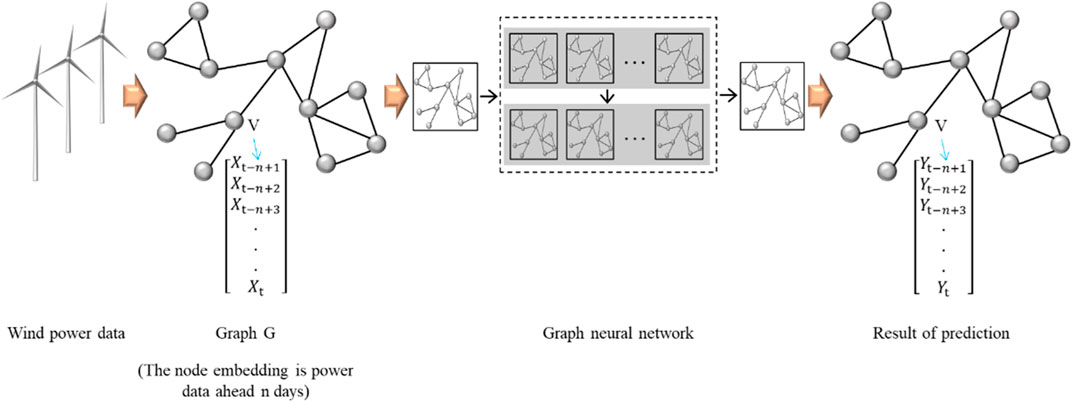
FIGURE 1. Schematic diagram of the graph neural network.

2.2 Deep Residual Network

In the practice of deep learning, there are problems in which the learning efficiency is lowered, and accuracy cannot be effectively improved owing to the deepening of the network. The essence of this problem is the loss of effective information caused by the deepening of the training process, commonly known as the network-degradation problem. In contrast to overfitting, this problem causes an overall decline in the training and testing accuracy.

He et al. (2016) proposed the DRN, a new network which provides an idea for effectively solving the problem of gradient disappearance when the network depth increases. A DRN can solve this problem in two ways, namely, identity mapping and residual mapping (Sun et al., 2020a; Sun et al., 2020b). If the network has reached the optimum and continues to deepen, the residual mapping will be pushed to 0, leaving only identity mapping. Thus, the network is in the optimal state, and its performance will not decrease with the deepening of the network.

During residual learning, input x passes through a few stacked nonlinear layers (Boroumand et al., 2018). Any desired mapping can be expressed as h(x), which can directly use a shortcut connection named identity mapping x, while the stacked nonlinear layers can be used to fit a residual mapping function F(x) = h(x) − x. Therefore, assuming that the two weight layers fit the residual function F(x), let h(x) = F(x) + x. In practice, the residual mapping F(x) are found to be easier to optimize than h(x). The details of the residual block are expressed as follows:

${\mathit{y}}_{\mathit{l}}=\mathit{h}\left({\mathit{x}}_{\mathit{l}}\right)+\mathit{F}\left({\mathit{x}}_{\mathit{l}},{\mathit{W}}_{\mathit{l}}\right)(1)$

${\mathit{x}}_{\mathit{l}+1}=\mathit{f}\left({\mathit{y}}_{\mathit{l}}\right)(2)$

where $x_l$ is the input of the lth block of the residual network and $x_{l+1}$ is the output. $h\left(x_l\right)=x_l$ denotes identity mapping and $f\left(\right)$ denotes the activation function.

Eq. 3 can be obtained recursively:

${\mathit{x}}_{\mathit{L}}={\mathit{x}}_{\mathit{l}}+{\displaystyle \sum }_{\mathit{i}=\mathit{l}}^{\mathit{L}-1}\mathit{F}\left({\mathit{x}}_{\mathit{i}},{\mathit{W}}_{\mathit{i}}\right)(3)$

The input of the Lth residual block can be expressed as the sum of the input of a shallow residual block and all the complex identity mappings. Introducing a loss function $\epsilon$, the parameter learning can be described as

$\frac{\mathit{\delta \epsilon }}{\mathit{\delta }{\mathit{x}}_{\mathit{l}}}=\frac{\mathit{\delta \epsilon }}{\mathit{\delta }{\mathit{x}}_{\mathit{L}}}\left(1+\frac{\mathit{\delta }}{\mathit{\delta }{\mathit{x}}_{\mathit{l}}}{\displaystyle \sum }_{\mathit{i}=\mathit{l}}^{\mathit{L}-1}\mathit{F}\left({\mathit{x}}_{\mathit{i}},{\mathit{W}}_{\mathit{i}}\right)\right)(4)$

Explicit modification of the network structure and residual mapping make it easier for the network to learn the optimal solution. In this study, the filter size and filter number were selected to optimize the computational performance.

2.3 Benchmark

In this study, three benchmarking machine learning algorithms, namely, neural network, support vector regression, and extreme learning machine, were compared with the proposed method in power prediction.

Neural networks (NN) are the underlying models of AI that have a wide range of applications in many fields (Ouyang et al., 2019a). The NN model with the backpropagation optimization mode was selected in this work. The number of hidden layers with values of 3, 4, and five and the number of hidden neurons in each hidden layer with values of 10, 20, 30, 40, and 50 were all evaluated in the training process via 10-fold cross validation. The activation function used in NN is the sigmoid function.

The (SVR) algorithm is used to find a regression plane and position all the data in a set closest to the plane (Li et al., 2020). The SVR parameters included the capacity factor C and $\gamma =1/2{\sigma }^2$. The values of C (1, 10, 100, 1,000, 10,000), and $\sigma$ (0.0001, 0.001, 0.01, 0.1, 1) were all evaluated in the training process via 10-fold cross-validation. The kernel function used in SVR is the RBF function.

An extreme learning machine (ELM) is a type of machine learning algorithm based on a single hidden layer feedforward neural network that is suitable for both supervised and unsupervised learning. The number of hidden neurons with values of 5, 10, 15, …, 100 were evaluated during the training process via 10-fold cross-validation. The activation function used in ELM is the sigmoid function (Li et al., 2018).

2.4 Evaluation Metrics

In this study, the mean square error (MSE) and coefficient of determination (R²) were used to assess the prediction accuracy of the proposed framework. Here, R² measures the percentage of the variance explained by the prediction outcome. It basically interprets what percentage of variance of the actual outcome are explained by the prediction outputs.

$\mathit{MSE}=\frac{1}{\mathit{n}}{\displaystyle \sum _{\mathit{i}=1}^{\mathit{n}}\left|\frac{{\mathit{y}}_{\mathit{i}}-\overline{{\mathit{y}}_{\mathit{i}}}}{{\mathit{y}}_{\mathit{i}}}\right|}(5)$

${\mathit{R}}^2=\frac{{\displaystyle \sum {\left(\overline{\mathit{y}}-\overline{{\mathit{y}}_{\mathit{i}}}\right)}^2}}{{\displaystyle \sum {\left(\overline{\mathit{y}}-{\mathit{y}}_{\mathit{i}}\right)}^2}}(6)$

where $y_i, \overline{y_i}, \overline{y}, and \text{n }$ represent the actual power, predicted power, average value of $y_i,$ and number of test datasets, respectively.

3 Case Study and Data Collection

The SCADA dataset used in this study was recorded at a wind farm named Kushui Wind Farm, which is located in the Gobi Desert in the east of the camel circle, approximately 120 km away from Hami City, Xinjiang, China. The wind farm is located in an alpine area at an altitude of 1,135—1,395 m that is rich in wind energy potential. The entire wind farm has many wind turbines distributed on open and flat terrain. Detailed information about the location is presented in Figure 2.

FIGURE 2

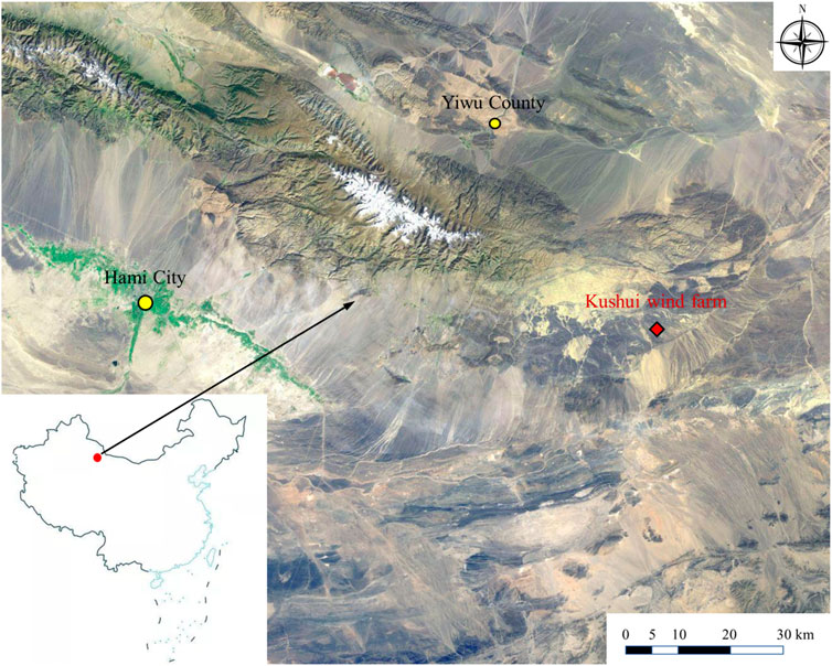
FIGURE 2. Location of the case study wind farm in Hami County, Xinjiang, China.

According to Table 1, the SCADA system collected datasets of individual wind turbines, usually including the wind speed (unit: m/s), wind direction (unit: rad), temperature (unit: °C), barometric pressure (unit: kPa), humidity (unit: %), and wind power (unit: kW). In this case, to predict the wind power, the inputs based on domain knowledge included the first five parameters above.

TABLE 1

TABLE 1. Summary of the dataset in the case study.

4 Results

4.1 GNN

In this section, extensive experiments are presented to validate the effectiveness of the proposed approach. The dataset utilized for the experiments was collected from a wind farm located in Hami, Xinjiang, China, and the data collected were obtained using the SCADA system. We select only the power-related SCADA variables, as listed in Table 1. In this study, we collected the SCADA variables from a single target turbine and the historic wind power from its adjacent turbines, which are the neighbors of the target turbine.

A heterogeneous graph was constructed among the six turbines to learn the unified representation power time series of the target turbine. In the graph, the measured real-time power from the target turbine was treated as the target node, and the historical power series from adjacent turbines were defined as the source nodes. Inner-modality attention and inter-modality attention were used to learn the different contributions of graph-structured sources to the target node. Weight values denote the correlation between the source and target nodes. After computing all the weights, a threshold of 0.5 was implemented to determine whether the link between the two nodes was worth retaining. In the final step, a learned graph structure was utilized to determine the number of inputs of wind power generated in adjacent turbines into the prediction model to forecast the power of the target turbine in the short term.

4.2 Hyper-Parameters of DRN

In this section, the hyper-parameters of DRN are studied. Three experiments were designed to evaluate the effect of the filter size on the computation, as well as four experiments for filter number. Owing to the limitations of the hardware, the filter sizes were set as 2 × 2, 3 × 3, and 4 × 4, while the filter numbers were set as 16, 32, 64, and 128.

For the filter size, the DRN is trained with a filter number of 16, which indicates that three reference computational results can be obtained during the validation set. Figure 3A shows that the maximum and minimum RMSE appear at the first and second filter sizes, respectively. The RMSE increases with the filter size. As shown in Figure 3B, the best R² of 0.958 is obtained when the filter size is 3 × 3.

FIGURE 3

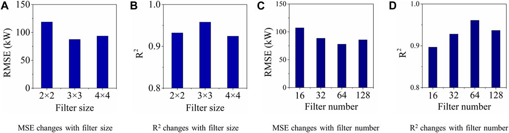
FIGURE 3. Tuning the filter size and filter number for DRN.

Next, a computation was conducted using a filter size of 3 × 3 and various values of the filter number, as mentioned above. Figure 3C shows that the RMSE decreases when filter number increases, and the optimal solution occurs when the filter number is 64, possibly owing to the overfitting of the model with continuously increasing filter numbers. Figure 3D provides the same evidence for the computation. Therefore, the best performance is achieved when the filter size and number are 3 × 3 and 64, respectively.

4.3 Wind Power Prediction

Experiments were performed with three selected algorithms were performed using two measurement metrics (RMSE and R²) to comprehensively evaluate the prediction performance of the proposed method. The hyperparameters of all the algorithms were tuned. In each training-validation experiment, the steps of input time and output time range were 1, 2, …, 20. In all the experiments conducted, the wind power was predicted for different input and output time steps. The relevant computational behavior is shown in Figure 4, which shows the correspondence between the predicted power obtained numerically and experimentally.

FIGURE 4

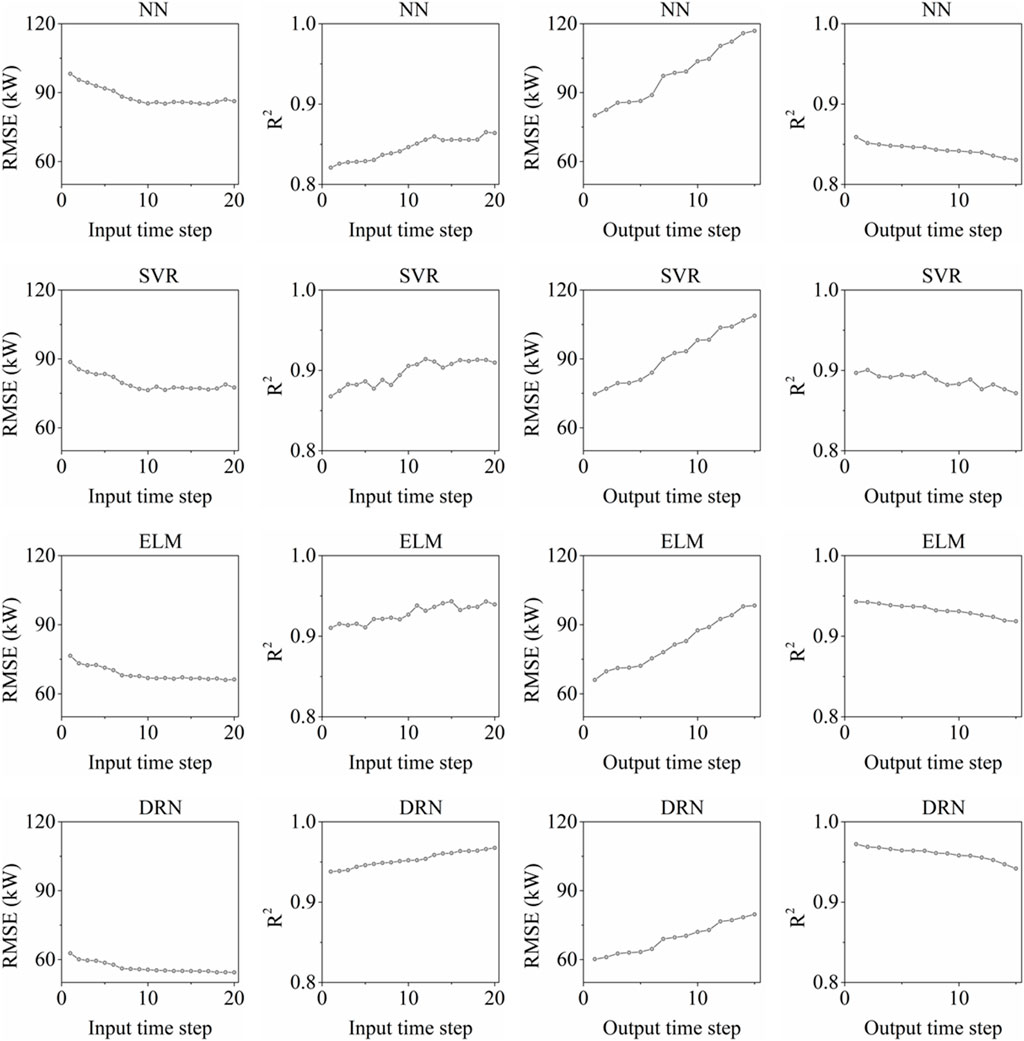
FIGURE 4. Impact of input/output size on the prediction performance.

According to Figure 4, the RMSE from all the algorithms decreases when the input time step increases, whereas it increases when the output time step increases. When the same length of historical data is input, longer the output steps yield larger prediction errors. Furthermore, a deeper analysis of the results for R² indicated good linearity between the predicted and measured wind power values and the error occurring in the long-term horizon of the output time step. The two measurement metrics yielded similar results. Overall, the computational results demonstrated that the proposed method based on DRN significantly outperformed the other three benchmarking machine learning algorithms, exhibiting the lowest RMSE and maximal R² with increasing input time step and output time step. The DRN exhibited its outperformance in terms of prediction in the temporal domain owing to its ability to handle redundant information.

Moreover, this study also investigated the influence of the size of the training samples on the prediction results. Three approaches based on NN, SVR, and ELM were adopted to demonstrate the superiority of the DRN model. The hyperparameters of all the algorithms were selected from previous results, and the data samples ranged from 400—4,000, at intervals of 200.

From Figure 5, it can be observed that the prediction performance varies with the training data size. As the training data size increases, the RMSE of NN decreases from 116.61 to 80.07 kW. The smallest RMSE values of SVR, ELM, and DRN were 74.74, 66.25 and 60.28 kW, respectively. The R² of the DRN increases from 0.941 to 0.976, and the maximal R² values of the other three algorithms were 0.862, 0.908, and 0.943, respectively. The computational results imply that the worst case result from DRN surpasses the other best cases. This phenomenon provides strong evidence for DRN optimization.

FIGURE 5

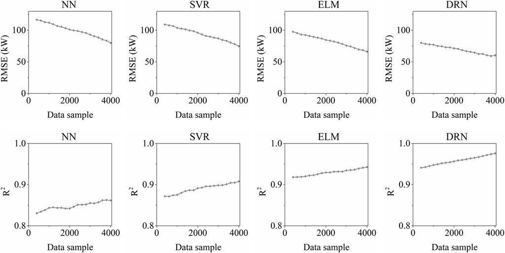
FIGURE 5. Impact of training sample size on the prediction performance.

Table 2 shows that the proposed DRN-based method produces the lowest prediction error and best prediction performance based on the case study presented. The mean values of the RMSE from NN, SVR, ELM, and DRN were 99.32, 88.26, 80.53, and 70.19, respectively. The Std. for the four methods are 10.79, 12.36, 10.46, and 5.93, respectively. For R², the mean value from DRN is 0.96, which possesses the most advantages compared to NN, SVR, and ELM. This phenomenon indicates that the proposed method for wind-power prediction is a statistical outlier and can be utilized to further improve related prediction tasks.

TABLE 2

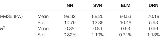
TABLE 2. Summary of the wind power forecasting performance.

5 Conclusion

In this study, we present a data-driven short-term wind power prediction framework that integrates GNN and DRN. GNN was used to obtain a graph structure to describe the correlation between the power of the target turbine and that generated by adjacent turbines. The DRN was trained to predict the short-term wind power. The SCADA variables, along with the power generation of adjacent turbines, were all considered as inputs of the forecasting model. A comparative analysis was conducted against other benchmark forecasting algorithms.

Computational results demonstrated that the graph structure can effectively capture the spatial-temporal relationships among adjacent turbines. Comparative analysis demonstrated that the DRN has superior power in short-term wind power forecasting. The proposed approach is expected to be useful to field engineers at wind farms. Ouyang et al., 2019c.

Data Availability Statement

The original contributions presented in the study are included in the article/Supplementary Material, further inquiries can be directed to the corresponding author.

Author Contributions

HL conceptualized the study, contributed to the study methodology, data curation, software and formal analysis, and wrote the original draft.

Funding

This research is supported by the “Miaozi project” of scientific and technological innovation in Sichuan Province, China (Grant No. 2021090) and the Opening fund of State Key Laboratory of Geohazard Prevention and Geoenvironment Protection (Chengdu University of Technology) (Grant No. SKLGP 2021K014).

Conflict of Interest

The author declares that the research was conducted in the absence of any commercial or financial relationships that could be construed as a potential conflict of interest.

Publisher’s Note

All claims expressed in this article are solely those of the authors and do not necessarily represent those of their affiliated organizations, or those of the publisher, the editors and the reviewers. Any product that may be evaluated in this article, or claim that may be made by its manufacturer, is not guaranteed or endorsed by the publisher.

References

Ait Maatallah, O., Achuthan, A., Janoyan, K., and Marzocca, P. (2015). Recursive Wind Speed Forecasting Based on Hammerstein Auto-Regressive Model. Appl. Energy 145, 191–197. doi:10.1016/j.apenergy.2015.02.032

CrossRef Full Text | Google Scholar

Bi, X., Liu, Z., He, Y., Zhao, X., Sun, Y., and Liu, H. (2020). GNEA: a Graph Neural Network with ELM Aggregator for Brain Network Classification. Complexity 2020. doi:10.1155/2020/8813738

CrossRef Full Text | Google Scholar

Boroumand, M., Chen, M., and Fridrich, J. (2018). Deep Residual Network for Steganalysis of Digital Images. IEEE Trans. Inf. Forensics Secur. 14 (5), 1181–1193. doi:10.1109/TIFS.2018.2871749

CrossRef Full Text | Google Scholar

Chen, C., Li, K., Teo, S. G., Zou, X., Wang, K., Wang, J., et al. (2019). Gated Residual Recurrent Graph Neural Networks for Traffic Prediction. Aaai 33 (1), 485–492. doi:10.1609/aaai.v33i01.3301485

CrossRef Full Text | Google Scholar

Chen, G., Li, L., Zhang, Z., and Li, S. (2020). Short-term Wind Speed Forecasting with Principle-Subordinate Predictor Based on Conv-Lstm and Improved Bpnn. IEEE Access 8, 67955–67973. doi:10.1109/access.2020.2982839

CrossRef Full Text | Google Scholar

Deo, R. C., Ghorbani, M. A., Samadianfard, S., Maraseni, T., Bilgili, M., and Biazar, M. (2018). Multi-layer Perceptron Hybrid Model Integrated with the Firefly Optimizer Algorithm for Windspeed Prediction of Target Site Using a Limited Set of Neighboring Reference Station Data. Renew. energy 116, 309–323. doi:10.1016/j.renene.2017.09.078

CrossRef Full Text | Google Scholar

Gori, M., Monfardini, G., and Scarselli, F. (2005). “A New Model for Learning in Graph Domainsconf,” in Proceedings. 2005 IEEE International Joint Conference on Neural Networks, 2005, 31 July-4 Aug. 2005, Montreal, QC, Canada 2 (2005), 729–734. doi:10.1109/IJCNN.2005.1555942

CrossRef Full Text | Google Scholar

Han, P., Li, Z., Liu, Y., Zhao, P., Li, J., Wang, H., et al. (2020). “Contextualized Point-Of-Interest Recommendation,” in Proceedings of the International Joint Conferences on Artificial Intelligence Organization, Yokohama Yokohama, Japan, January 2020. doi:10.24963/ijcai.2020/344

CrossRef Full Text | Google Scholar

Han, Q., Meng, F., Hu, T., and Chu, F. (2017). Non-parametric Hybrid Models for Wind Speed Forecasting. Energy Convers. Manag. 148, 554–568. doi:10.1016/j.enconman.2017.06.021

CrossRef Full Text | Google Scholar

He, K., Zhang, X., Ren, S., and Sun, J. (2016). “Deep Residual Learning for Image Recognition,” in Proceedings of the IEEE conference on computer vision and pattern recognition, Las Vegas, NV, USA, June 2016, 770–778. doi:10.1109/cvpr.2016.90

CrossRef Full Text | Google Scholar

He, Y., and Kusiak, A. (2017). Performance Assessment of Wind Turbines: Data-Derived Quantitative Metrics. IEEE Trans. Sustain. Energy 9 (1), 65–73. doi:10.1109/TSTE.2017.2715061

CrossRef Full Text | Google Scholar

Huang, H., Liu, F., Zha, X., Xiong, X., Ouyang, T., Liu, W., et al. (2018). Robust Bad Data Detection Method for Microgrid Using Improved ELM and DBSCAN Algorithm. J. Energy Eng. 144 (3), 04018026. doi:10.1061/(asce)ey.1943-7897.0000544

CrossRef Full Text | Google Scholar

Kavasseri, R. G., and Seetharaman, K. (2009). Day-ahead Wind Speed Forecasting Using F-ARIMA Models. Renew. Energy 34 (5), 1388–1393. doi:10.1016/j.renene.2008.09.006

CrossRef Full Text | Google Scholar

Kumar, Y., Ringenberg, J., Depuru, S. S., Devabhaktuni, V. K., Lee, J. W., Nikolaidis, E., Andersen, B., and Afjeh, A. (2016). Wind Energy: Trends and Enabling Technologies. Renew. Sustain. Energy Rev. 53, 209–224. doi:10.1016/j.rser.2015.07.200

CrossRef Full Text | Google Scholar

Lee, G., Ding, Y., Genton, M. G., and Xie, L. (2015). Power Curve Estimation with Multivariate Environmental Factors for Inland and Offshore Wind Farms. J. Am. Stat. Assoc. 110 (509), 56–67. doi:10.1080/01621459.2014.977385

CrossRef Full Text | Google Scholar

Li, H., Deng, J., Feng, P., Pu, C., Arachchige, D. D. K., and Cheng, Q. (2021a). Short-Term Nacelle Orientation Forecasting Using Bilinear Transformation and ICEEMDAN Framework. Front. Energy Res. 9, 780928. doi:10.3389/fenrg.2021.780928

CrossRef Full Text | Google Scholar

Li, H., Deng, J., Yuan, S., Feng, P., and Arachchige, D. D. K. (2021b). Monitoring and Identifying Wind Turbine Generator Bearing Faults Using Deep Belief Network and EWMA Control Charts. Front. Energy Res. 9, 799039. doi:10.3389/fenrg.2021.799039

CrossRef Full Text | Google Scholar

Li, H., He, Y., Xu, Q., Deng, j., Li, W., and Wei, Y. (2022). Detection and Segmentation of Loess Landslides via Satellite Images: a Two-phase Framework. Landslides 19, 673–686. doi:10.1007/s10346-021-01789-0

CrossRef Full Text | Google Scholar

Li, H., Xu, Q., He, Y., and Deng, J. (2018). Prediction of Landslide Displacement with an Ensemble-Based Extreme Learning Machine and Copula Models. Landslides 15 (10), 2047–2059. doi:10.1007/s10346-018-1020-2

CrossRef Full Text | Google Scholar

Li, H., Xu, Q., He, Y., Fan, X., and Li, S. (2020). Modeling and Predicting Reservoir Landslide Displacement with Deep Belief Network and EWMA Control Charts: a Case Study in Three Gorges Reservoir. Landslides 17 (3), 693–707. doi:10.1007/s10346-019-01312-6

CrossRef Full Text | Google Scholar

Liu, H., Mi, X., and Li, Y. (2018). Smart Multi-step Deep Learning Model for Wind Speed Forecasting Based on Variational Mode Decomposition, Singular Spectrum Analysis, LSTM Network and ELM. Energy Convers. Manag. 159, 54–64. doi:10.1016/j.enconman.2018.01.010

CrossRef Full Text | Google Scholar

Long, H., Li, P., and Gu, W. (2020). A Data-Driven Evolutionary Algorithm for Wind Farm Layout Optimization. Energy 208, 118310. doi:10.1016/j.energy.2020.118310

CrossRef Full Text | Google Scholar

Long, H., Xu, S., and Gu, W. (2022). An Abnormal Wind Turbine Data Cleaning Algorithm Based on Color Space Conversion and Image Feature Detection. Appl. Energy 311, 118594. doi:10.1016/j.apenergy.2022.118594

CrossRef Full Text | Google Scholar

Long, H., Zhang, C., Geng, R., Wu, Z., and Gu, W. (2021). A Combination Interval Prediction Model Based on Biased Convex Cost Function and Auto-Encoder in Solar Power Prediction. IEEE Trans. Sustain. Energy 12 (3), 1561–1570. doi:10.1109/tste.2021.3054125

CrossRef Full Text | Google Scholar

Luo, D., Cheng, W., Xu, D., Yu, W., Zong, B., Chen, H., et al. (2020). Parameterized Explainer for Graph Neural Network. Adv. neural Inf. Process. Syst. 33, 19620–19631. doi:10.48550/arXiv.2011.04573

CrossRef Full Text | Google Scholar

Mezaache, H., Bouzgou, H., and Raymond, C. (2016). “Kernel Principal Components Analysis with Extreme Learning Machines for Wind Speed Prediction,” in Proceedings of the Seventh International Renewable Energy Congress, IREC2016, March 2016, Hammamet, Tunisia.

Google Scholar

Ouyang, T., Zha, X., Qin, L., He, Y., and Tang, Z. (2019a). Prediction of Wind Power Ramp Events Based on Residual Correction. Renew. Energy 136, 781–792. doi:10.1016/j.renene.2019.01.049

CrossRef Full Text | Google Scholar

Ouyang, T., He, Y., Li, H., Sun, Z., and Baek, S. (2019b). Modeling and Forecasting Short-Term Power Load with Copula Model and Deep Belief Network. IEEE Trans. Emerg. Top. Comput. Intell. 3 (2), 127–136. doi:10.1109/tetci.2018.2880511

CrossRef Full Text | Google Scholar

Ouyang, T., Pedrycz, W., Reyes-Galaviz, O. F., and Pizzi, N. J. (2019c). Granular Description of Data Structures: A Two-phase Design. IEEE Trans. Cybern. 51 (4), 1902–1912. doi:10.1109/TCYB.2018.2887115

PubMed Abstract | CrossRef Full Text | Google Scholar

Ouyang, T., Pedrycz, W., and Pizzi, N. J. (2019d). Rule-based Modeling with DBSCAN-Based Information Granules. IEEE Trans. Cybern. 51 (7), 3653–3663. doi:10.1109/TCYB.2019.2902603

PubMed Abstract | CrossRef Full Text | Google Scholar

Ouyang, T., Kusiak, A., and He, Y. (2017). Modeling Wind-Turbine Power Curve: A Data Partitioning and Mining Approach. Renew. Energy 102, 1–8. doi:10.1016/j.renene.2016.10.032

CrossRef Full Text | Google Scholar

Scarselli, F., Gori, M., Tsoi, A. C., Hagenbuchner, M., and Monfardini, G. (2008). The Graph Neural Network Model. IEEE Trans. Neural Netw. 20 (1), 61–80. doi:10.1109/TNN.2008.2005605

PubMed Abstract | CrossRef Full Text | Google Scholar

Shen, X., Ouyang, T., Yang, N., and Zhuang, J. (2021). Sample-Based Neural Approximation Approach for Probabilistic Constrained Programs. IEEE Trans. Neural Netw. Learn. Syst. 1-8. doi:10.1109/tnnls.2021.3102323

CrossRef Full Text | Google Scholar

Shen, X., Zhang, Y., Sata, K., and Shen, T. (2020). Gaussian Mixture Model Clustering-Based Knock Threshold Learning in Automotive Engines. IEEE/ASME Trans. Mechatron. 25 (6), 2981–2991. doi:10.1109/tmech.2020.3000732

CrossRef Full Text | Google Scholar

Sun, Z., He, Y., Gritsenko, A., Lendasse, A., and Baek, S. (2020a). Embedded Spectral Descriptors: Learning the Point-wise Correspondence Metric via Siamese Neural Networks. J. Comput. Des. Eng. 7 (1), 18–29. doi:10.1093/jcde/qwaa003

CrossRef Full Text | Google Scholar

Sun, Z., Rooke, E., Charton, J., He, Y., Lu, J., and Baek, S. (2020b). Zernet: Convolutional Neural Networks on Arbitrary Surfaces via Zernike Local Tangent Space Estimation. Comput. Graph. Forum 39 (6), 204–216. doi:10.1111/cgf.14012

CrossRef Full Text | Google Scholar

Tang, Z., Li, Y., Chai, X., Zhang, H., and Cao, S. (2020). Adaptive Nonlinear Model Predictive Control of Nox Emissions under Load Constraints in Power Plant Boilers. J. Chem. Eng. Jpn. 53 (1), 36–44. doi:10.1252/jcej.19we142

CrossRef Full Text | Google Scholar

Ulazia, A., Sáenz, J., Ibarra-Berastegi, G., González-Rojí, S. J., and Carreno-Madinabeitia, S. (2019). Global Estimations of Wind Energy Potential Considering Seasonal Air Density Changes. Energy 187, 115938. doi:10.1016/j.energy.2019.115938

CrossRef Full Text | Google Scholar

Wan, J., Liu, J., Ren, G., Guo, Y., Yu, D., and Hu, Q. (2016). Day-ahead Prediction of Wind Speed with Deep Feature Learning. Int. J. Pattern Recognit. Artif. Intell. 30 (5), 1650011. doi:10.1142/s0218001416500117

CrossRef Full Text | Google Scholar

Wang, J., Wang, S., and Yang, W. (2019). A Novel Non-linear Combination System for Short-Term Wind Speed Forecast. Renew. Energy 143, 1172–1192. doi:10.1016/j.renene.2019.04.154

CrossRef Full Text | Google Scholar

Wang, Y., Wang, J., and Wei, X. (2015). A Hybrid Wind Speed Forecasting Model Based on Phase Space Reconstruction Theory and Markov Model: A Case Study of Wind Farms in Northwest China. Energy 91, 556–572. doi:10.1016/j.energy.2015.08.039

CrossRef Full Text | Google Scholar

Yin, H., Dong, Z., Chen, Y., Ge, J., Lai, L. L., Vaccaro, A., et al. (2017). An Effective Secondary Decomposition Approach for Wind Power Forecasting Using Extreme Learning Machine Trained by Crisscross Optimization. Energy Convers. Manag. 150, 108–121. doi:10.1016/j.enconman.2017.08.014

CrossRef Full Text | Google Scholar

Yunus, K., Thiringer, T., and Chen, P. (2015). ARIMA-based Frequency-Decomposed Modeling of Wind Speed Time Series. IEEE Trans. Power Syst. 31 (4), 2546–2556.

Google Scholar