Sparse Dictionary Learning for Transient Stability Assessment

1 Introduction

In power system stability studies, transient stability of a power system usually refers to the ability of the synchronous machines to remain in synchronism after a large disturbance (Kundur et al., 2004). Due to the increasing penetration of electricity demand and the integration of renewable energies, the power system’s dynamic characteristics are becoming more and more complex. The demand for dynamic security assessment of power systems is increasing. Transient stability assessment (TSA) is part of the dynamic security assessment of power systems, which involves evaluating the ability of a power system to remain in equilibrium under severe but credible contingencies. Therefore, TSA has been considered one of the main challenges and played a critical role in ensuring the reliability and stability of the power system’s operation.

Typically, the main approach used to solve the TSA can be summarized into three different categories: time-domain simulation method (Scala et al., 1998), direct method (Kakimoto et al., 1984), and artificial intelligence (AI) method (You et al., 2013; Wang et al., 2016). The basic idea for the time-domain simulation method is to solve the differential-algebraic equations (DAEs) of the power system. The time-domain simulation method has been widely used in the past decades because of its good performance on reliability. Scala et al. (1998) introduced a time-domain simulation method that solves the state-space differential equations to obtain the detailed dynamic behaviors of the power systems. Chan et al. (2002) presented a new development in online transient stability assessment and control using the time-domain simulation method. From the assessment results shown in the aforementioned study, the proposed approaches have a good stability accuracy rate, but it is also easy to find that the calculation results highly depend on the system model and parameters which means the computational effort is at a high level.

The principle of the direct method refers to constructing an energy function including the Lyapunov method (Kakimoto et al., 1984), transient energy function (TEF) method (Vittal et al., 1989), and extended equal area criterion (EEAC) method (Xue et al., 1989; Huang and Wang, 2019) to describe the transient stability of power systems. This method can provide a relatively fast response and a good accuracy rate when not solving the differential state-space equations. Vittal et al. (1989) introduced an approach using transient energy function (TEF) which consists of determining sensitivity coefficients and the development of the dynamic sensitivity equations. Xue et al. (1989) revealed the role of the extended equal area criterion (EEAC) method. This method aims to extract essential information out of a robust simulation and show the improvements and extensions that enhance the EEAC accuracy and its capability. Transient stability assessment of a stochastic multi-machine system based on EEAC is proposed by Huang and Wang (2019). The numerical simulation is based on the Monte Carlo method, and the simplicity and effectiveness are verified in the end. To summarize, the advantage of the direct method is the quick response and its ability to provide a stable margin, but it requires a large number of calculations since the energy function is difficult to construct.

In recent years, the development and value of artificial intelligence technologies have been widely recognized around the world. Compared with the conventional TSA methods, the utilization of artificial intelligence technology applied to TSA provided new perspective methods such as neural network (Bahbah and Girgis, 2004; Gupta et al., 2017) and support vector machine (SVM) (You et al., 2013; Hu et al., 2018). Gupta et al. (2017) presented an online monitoring system using a GRU-based RNN, which continuously predicts the current status based on the past data. Wang et al. (2021a) proposed an ensemble machine learning approach (multi-layer support vector machine model) to help improve the transient stability assessment during fault events. In addition, some of the previous works develop different feature selection methods for AI-based TSA. Li and Yang (2017) proposed a novel pattern recognition–based transient stability assessment (PRTSA) approach based on an ensemble of OS-extreme learning machines (EOSELM) by using the binary Jaya algorithm to select the optimal features with the use of phasor measurement unit (PMU) data. The experimental results show that the proposed method has superior computation speed and prediction accuracy. The basic idea of AI approaches is to build an AI-based assessment model of the power system’s operational parameters as input to evaluate the stability of the power system. In other words, the AI method can be considered a classification problem. By establishing the nonlinear mapping relationship between the data in a short time and the strong learning ability, the AI method exhibits a good performance in improving the assessment precision and accelerating the computation speed. Table 1 shows the principles, pros, and cons of different kinds of TSA methods (Zhang et al., 2021).

TABLE 1

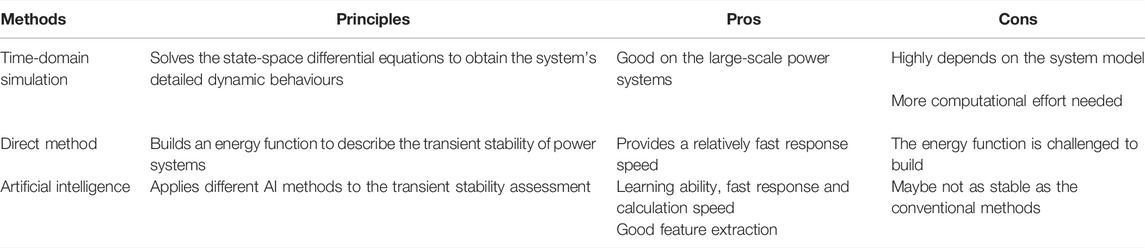
TABLE 1. Pros and cons of difference AI methods.

Although these AI methods have gained much popularity and success, the most important part of implementing the efficiency is the feature selection and optimization that have different sensitivities to condition changes (Liu et al., 2014). Based on the study by Wang et al. (2021b), the SVM can only achieve accurate classification results in a small sample space due to the structural risk minimization principle. Moreover, in the data training process, for example, the optimization parameters for certain classifiers in the SVM, such as the radial basis kernel function, is a key step to acquire significant accuracy, which increases the complexity of the procedure. In other words, the object and extracted features usually change, affecting the classifier’s performance. For GRU, it is very important to determine the weight matrices and bias vector so that the update gate and reset gate can get rid of the useless information delivered, which no doubt increases the complexity of the model. Thus, the development and improvement of AI technologies for simplifying the feature selection and the classification model is necessary. In some recently reported ideas, the sparse dictionary learning that uses the sparse representation of connected neural networks based on the sparse coding approach developed has been suggested to address the concerns mentioned earlier.

In general, the basic idea of sparse dictionary learning is finding a sparse representation of the input data to form a linear combination of basic elements. These elements combined with the original elements themselves are called atoms, and they are used to compose a dictionary. In other words, sparse representation represents the natural signals by a sparse linear combination of atoms in a fixed dictionary (Donoho et al., 2006). Sparse signals are characterized by non-zero coefficients in one of their transformation domains (Stanković et al., 2019). Sparse dictionary learning has attracted widespread attention in real-world applications such as signal processing and in power system areas. For example, Akhavan et al. (2022) investigated the dictionary learning problem for sparse representation when there is hidden Markov model dependency among the training signals, and the proposed approach improves the performance of the dictionary learning algorithms in the mentioned scenario. Dictionary learning sparse decomposition is implemented by Cai et al. (2019) for a highly accurate and fast quality disturbance classification. The results demonstrate that the dictionary learning method has good improvement in computational complexity and classification accuracy. In the study by Ren et al. (2016), a joint model of sparse-representation-based and SVM on fault diagnosis approach is proposed to compute the sub-dictionaries and represent the testing sample.

The literature reviews aforementioned established a clear point of view that the dictionary-based learning approach in power systems has been successfully applied to signal processing, power quality disturbance classification, and fault diagnosis. Therefore, the main contribution of this study is applying the sparse dictionary learning approach to transient stability assessment to improve the precision of the classification accuracy of TSA in power systems. Furthermore, this study investigates performance comparisons of TSA using multi-layer support vector machine (ML-SVM) and long short-term memory network–based recurrent neural network (LSTM). The proposed method exhibits satisfactory classification accuracy in transient stability prediction and provides the ability to reduce false alarms both in positives and negatives of the power system. The data are obtained by simulating thousands of different time-domain simulation (TDS) scenarios which are performed on the New-England 39-bus system in the PSAT (power system analysis toolbox). The K-SVD approach is used to develop stable and unstable dictionaries.

The rest of this article is organized as follows: Section 2 presents the basic idea of sparse representation theory and the K-SVD algorithm. Section 3 introduces the philosophy of the proposed dictionary learning TSA method. Section 4 is the case study using different AI technologies. The simulation and results are given in Section 5. The last part of the article is the conclusion.

2 Theoretical Background

2.1 Sparse Representation Theory

In recent years, sparse representation theory has attracted more attention. We simply consider dictionary learning a method of learning a matrix which is called a dictionary such that we can write a signal as a linear combination of as few columns from the matrix as possible. Generally speaking, the basic idea of sparse dictionary learning is finding a sparse representation of the input data to form a linear combination of basic elements. These elements combined with the original elements themselves are then called atoms to compose a dictionary. In other words, sparse representation represents the natural signals by a sparse linear combination of atoms in a fixed dictionary (Donoho et al., 2006). The basic model of this method is illustrated in Figure 1. As mentioned previously, the model assumes that a digital signal is represented as a sparse linear combination of atoms obtained from a fixed dictionary. Atoms in the dictionary can be an over-complete spanning set, not to be orthogonal strictly. For an input signal $\mathit{y}\mathrm{\in }{\mathit{R}}^{\mathit{m}\times \mathit{n}}$ (m is the number of the samples and $n$ is the property of the samples $),$ the expression is $y=\mathit{D}x$, where $\mathit{D}\mathrm{\in }{\mathit{R}}^{\mathit{m}\times \mathit{k}}$ is the dictionary and $x\in R^{K\times m}$ is the sparse matrix. The dictionary matrix $\mathit{D}$ contains $K$ atoms, where $d_k\in R^m,$ $k=1, 2, \cdots K$ are its columns (Han et al., 2018). If $m<K$, the dictionary is over-complete. When the dictionary $\mathit{D}$ and input signal $y$ are fixed, we will obtain the sparsest representation matrix, in which the majority of the entries in the sparse matrix are zero.

FIGURE 1

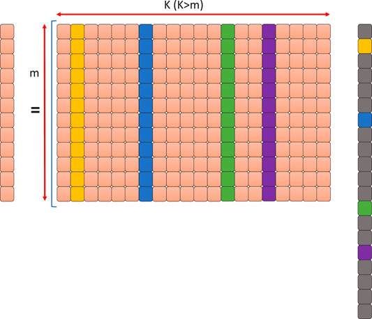
FIGURE 1. Basic model of sparse representation theory.

The dictionary learning algorithm is usually formulated as the following optimization problem.

${min}_x{\Vert x\Vert }_{0}s.t.y=\mathit{D}x,(1)$

where ${\Vert \cdot \Vert }_0$ is the $l_0$ pseudo-norm, which represents the number of non-zeros entries in the sparse matrix $x$. Our goal is to find $x$ such that the error $y-\mathit{D}{x}_2$ is small. That means $x$ has to be as sparse as it could be so that we only use a few of the available atoms in the dictionary. We could try to minimize the error aforementioned to get a sparse $x$, but in most certain works, it is hard to achieve since the equality constraint $y-\mathit{D}x$ is too strict. Therefore, we add $l_0$-regularization with a threshold $\epsilon$, and the optimization problem becomes

$\left(P_{0,\epsilon }\right){min}_x{\Vert x\Vert }_{0}s.t.{\Vert y-{\mathit{D}}_x\Vert }_2\le \epsilon ,(2)$

where $\epsilon$ depends on the noise level of the signal. The optimization process is called sparse coding. The corresponding unconstrained form of the aforementioned equation can be represented using the Lagrange multipliers as

$\left(P_{0,\lambda }\right){min}_x \frac{1}{2}\Vert y-\mathit{D}x\Vert \frac{2}{2}+\lambda \Vert {x\Vert }_0.(3)$

The approaches provided earlier can obtain an approximate solution that is not globally optimal because Eqs. 1, 2 are underdetermined system equations. This is a combinational optimization problem, and the process is a non-deterministic polynomial (NP) hard problem. To solve this, in the past few decades, several efficient approximate solutions are proposed in practice. Generally, these methods can be divided into two main categories: greedy algorithm and relaxation algorithm. For greedy algorithms, matching pursuit (MP) (Mallat and Zhang, 1993) and orthogonal matching pursuit (OMP) (Chen et al., 1989) are widely used to select the dictionary atoms sequentially based on the correlation between the columns of the dictionary and the input signal to compute the inner products.

For the relaxation algorithm, basis pursuit (BP) (Chen et al., 2001) is another well-known algorithm in this category. BP converts Eqs. 1, 2 to their convex counterparts by replacing the $l_0$ pseudo-norm with $l_1$ pseudo-norm.

$\left(P_{1,\epsilon }\right)mi{n}_x{\Vert x\Vert }_{1}s.t.{\Vert y-{\mathit{D}}_x\Vert }_2\le \epsilon ,(4)$

where ${\Vert \cdot \Vert }_1$ is the $l_1$ pseudo-norm. Compared to the $l_0$ pseudo-norm, the $l_1$ pseudo-norm has a better mathematical performance to serve as the objective function of the optimization model. The corresponding unconstrained form of the aforementioned equation can be represented using the Lagrange multipliers as

$\left(P_{1,\lambda }\right){min}_x \frac{1}{2}{\Vert y-\mathit{D}x\Vert }_2^2+\lambda {\Vert x\Vert }_1.(5)$

$x$ tends to be sparser when $\lambda$ becomes larger, so fewer dictionaries are obtained.

2.2 K-Singular Value Decomposition Algorithm

In sparse representation, the K-singular value decomposition (K-SVD) algorithm (Aharon et al., 2006) is a highly effective method for training over-complete dictionaries (Rubinstein et al., 2012). The purpose of the sparse dictionary learning method is to choose a suitable dictionary. Predesigned transform such as the wavelet (Mallat, 1999), curvelet (Candes and Donogo, 2000), or contourlet transforms (Do and Vetterli, 2006) is one of the methods to emerge from the dictionary. The other method is finding the dictionary from the input data using training process. The K-SVD algorithm is a type of data training technique to train the dictionary. The high efficiency makes it successfully applied in several image processing tasks (Elad and Aharon, 2006; Mairal et al., 2008; Protter and Elad, 2008).

The K-SVD algorithm accepts an initial over-complete dictionary ${\mathit{D}}_0$, a number of iterations $k$, and a set of training signals arranged as the columns of the matrix $X$. In general, the purpose of the K-SVD algorithm is to improve the dictionary iteratively to make the representation of the signals as sparse as it could be in the matrix $X$ by solving the following optimization problem:

${min}_{\mathit{D},\mathrm{\Gamma }}{\Vert X-\mathit{D}\mathrm{\Gamma }\Vert }_F^2 s.t. \forall {\Vert {\gamma }_i\Vert }_0\le K,(6)$

where $\gamma$ is the sparse representation and $K$ is the target sparsity. There are two basic steps involved in the K-SVD algorithm to constitute the algorithm iteration:

1) The signals in $X$ are sparse-coded given the current dictionary estimate, producing the sparse representation matrix $\text{Γ}$;

2) The dictionary atoms are updated given the current sparse representation.

Line 4 of the pseudocode in Table 2 shows the sparse coding part which is commonly implemented using OMP. The second loop between line 5 to line 12 indicates the updated dictionary which is performed using one atom each time and individually optimizes the target function for each atom. The rest of the atoms are kept fixed (Rubinstein et al., 2012).

TABLE 2

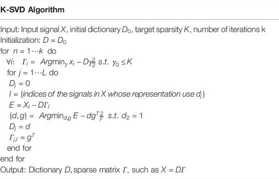
TABLE 2. Pseudocode of K-SVD algorithm.

The innovation of the algorithm is to update the atom which is utilized while preserving the constraint in Eq. 6. To achieve this, the update step uses only the signals in $X$ whose sparse representation uses the current atom. I denotes the index of the signals in $X$ which uses the $j^{th}$ atom. The optimization of the target function is

${\Vert X_{\mathit{I}}-\mathit{D}{\mathrm{\Gamma }}_{\mathit{I}}\Vert }_F^2.(7)$

The problem is a rank-1 approximation task by

$\left\{d,g\right\}=Arg{min}_{d,g} {\Vert \mathit{E}-d{g}^T\Vert }_F^{2}s.t.{\Vert d\Vert }_2=1,(8)$

where $E=X_I-{\displaystyle \sum _{i\ne j}{d}_i{\mathrm{\Gamma }}_{i,I}}$ is the error matrix without the $j^{th}$ atom, $d$ is the updated atom, and $g^T$ is the new coefficients row in ${\text{Γ}}_I$.

3 Sparse Dictionary Learning TSA Model

3.1 Top–Down Philosophy of the Sparse Dictionary Learning Transient Stability Assessment Model

By determining the relative generator rotor angles, the stability of the system can be analyzed. Figure 2 describes the top–down philosophy of the proposed sparse dictionary learning TSA method.

FIGURE 2

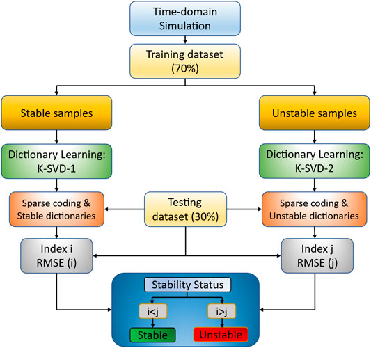
FIGURE 2. Top–down philosophy of sparse dictionary learning–based TSA.

The data samples will be divided into training datasets for dictionary learning and testing datasets for evaluation. For the dictionary learning part, in order to obtain the fittest sparse dictionary, the training dataset is separately labeled into two datasets: stable and unstable. The stable dataset is used as input data for implementing the stable dictionaries ${\mathit{D}}_{\mathit{s}}$, and the unstable dataset is used as input data for establishing unstable dictionaries ${\mathit{D}}_u$. The K-SVD algorithm is used to develop the sparse dictionaries.

The testing dataset contains both stable and unstable samples. The stable and unstable sparse coding $X_s$ and $X_u$ are individually stepped into the learned dictionary ${\mathit{D}}_s$ and ${\mathit{D}}_u$ to determine the stability status of the system, respectively. Two indexes are used to determine the stability status: if the RMSE index of the output in the stable dictionary $RMSE\left(i\right)$ is less than that of the unstable dictionary $RMSE\left(j\right)$, then the system is considered stable. In the opposite direction, the system is targeted as being unstable. By applying these analysis criteria, the classification accuracy, the reliability (false positive success rate), and security (true negative success rate) can be evaluated.

3.2 Transient Stability Assessment Performance

Not only the classification accuracy should be outlined but also the following evaluation indexes are necessary to be considered. The confusion matrix in Table 3 can better evaluate the proposed model not only using the accuracy.

TABLE 3

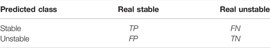
TABLE 3. Confusion matrix for TSA classification.

$TP$ is true positive, indicating the number of stable samples correctly predicted; $FP$ is false positive, which means the number of unstable samples incorrectly predicted; $FN$ means false-negative, which represents the number of stable samples but mispredicted; and $TN$ is true-negative, which is the number of unstable samples correctly predicted. In order to evaluate the performance of the proposed TSA model comprehensively, the following indexes are calculated:

The A index is the accuracy, which defines the ability of the method to correctly classify the testing samples compared to the observed data:

$A(\%)=\frac{TP+TN}{TP+TN+FN+FP}.(9)$

The $R_u$ index allows for evaluating the performance of misjudging the unstable sample as a stable one. As once, this situation happens in a power system, and it may lead to a large electricity blackout. In other words, if the classification results consider an unstable case as a stable one, no further action will be taken, which will destroy the operation of the system. Therefore, the $R_u$ index could ensure the reliability of the system.

$R_u(\%)=\frac{TN}{TN+FP}.(10)$

The $R_s$ index is used to evaluate the prediction of stable samples. Once the classification results mispredict the stable cases as unstable ones, the operator needs to take action to clear the fault. But actually, there is no fault occurring at the moment. Therefore, the $R_s$ index is used to ensure the security of the system.

$R_s(\%)=\frac{TP}{TP+FN}.(11)$

4 Case Studies

Wang et al. (2021a) conducted a transient stability assessment using the multi-layer support vector machine (ML-SVM) method. Figure 3 shows the framework of the method. The “Classifier” module on the left processes all the input data to the feature selection stage. With different feature subsets, ML-SVM trains and tests that information separately. Then, all different classification results are integrated together to represent the system’s stability in the “Integrated TSA” part.

FIGURE 3

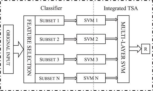
FIGURE 3. Framework of ML-SVM based TSA.

A genetic algorithm (Xiang et al., 2007) is used to perform the feature selection. The simulation is carried out on the IEEE 9-bus system in PowerWorld simulator. A three-phase fault sets on bus 7 at $t$ = 1.0 s and clears at $t=$ 1.077 s. In total, 30 input features are selected for the simulation process. By changing the generator and load levels in a specific range, a total of 1,000 samples are generated from the time-domain simulation. To validate the efficiency, 800 of them are the training set and 200 of them are used as the testing set. Transient stability is determined by the relative rotor angles of the generators. The result shows that the proposed advanced SVM method has a 93% classification accuracy.

In the study by Wang et al. (2021b), the authors propose a transient stability prediction method based on the long short-term memory (LSTM) network (Hochreiter and Schmidhuber, 1997). The detailed schematics of an LSTM block is illustrated in Figure 4. As shown in the figure, a cell state, input gate, forget gate, and output gate compose a general LSTM unit. The forget gate is used to control what information in the past state needs to be discarded. Then, the selected information is delivered to the current state. Each LSTM block connects to the following block directly in a sequence to form the LSTM network module. The initial state is the preset input from the system. The input to the next block consists of the hidden states from the previous block layer.

FIGURE 4

FIGURE 4. Architecture of an LSTM block.

To validate the proposed method, the New-England 39-bus system is adopted, and the simulation assumes that a three-phase fault occurs at bus 31 at $t$ = 1.0 s and is cleared at $t$ = 1.08 s. Different levels of generators and loads based on the power flow are generated, and the relative rotor angles are used to determine the transient stability of the system. Compared to the results from the previous case study, the classification accuracy of the LSTM method improved by 4%, which increased to 97%.

5 Simulation and Results

5.1 Model

For the purpose of evaluating the efficiency of the proposed approach, the same simulation model in Section 4 has been applied as a benchmark. Figure 5 shows the one-line diagram of the classical New-England 39-bus system (Padiyar, 1990). The New-England 39-bus system consists of 10 generators and 21 loads.

FIGURE 5

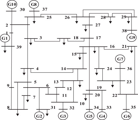
FIGURE 5. One-line diagram of the New-England 39-bus system.

To make the best diversity of the sample data, the disturbance considered is three-phase short-circuit faults at bus 31 with various locations at 20%, 40%, 60%, and 80% of the transmission line length. The faults are set at a time equal to 1 s, and the fault clears after 0.08 s. Fault samples are selected by N-1 accident. The duration of the simulation is 5 s. The fault is repeated at different generator levels and loading levels (the range of the level varies between 80% and 120% of the rating values by an increment of 10%). All the simulation data are generated by performing the time-domain simulation in PSAT (Milano, 2005) with the MATLAB platform. In terms of the model settings, the fault samples are 6,355 with different input features. Due to the longer time to display the change of the generator’s rotor speed, the generator’s rotor angle reflects faster to evaluate the stability of the system (Gomez et al., 2011). Therefore, the stability is denoted based on the transient stability index (TSI) calculated in terms of the relative generator rotor angles. The TSI index is defined as

$\eta =360°-{\left|\mathrm{\Delta }\delta \right|}_{\mathit{max}},(12)$

where ${\left|\mathrm{\Delta }\delta \right|}_{max}$ is the absolute value of the maximum rotor angle difference between any two generators after the fault is removed.

5.2 Input Features and Data Training

To evaluate the model properly, the input features need to fully reflect the dynamic behavior of the system. The case studies in Section 4 have further proved that the bus voltage and angle can accurately represent the system’s behavior. In addition, the node dynamic variables such as active and reactive power both on generators and loads, which reflect the system dynamics, are also used to generate the input features of TSA. There are a total of 140 features including active and reactive power of generators (No. 1–20), bus voltage and angle (No. 21–98), and active and reactive power of the loads (No. 99–140). Table 4 shows the detailed features of the input dataset.

TABLE 4

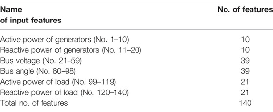
TABLE 4. Input features.

In the data training process, both the OMP and K-SVD implementations are made using the platform of MATLAB with OMP-Box v10 and KSVD-Box v13 (Rubinstein et al., 2008). The K-SVD toolbox uses the K-SVD algorithm to recover the dictionary, and the convergence of the K-SVD target function and the fraction of the recovered atoms are computed.

Hyperparameters such as the ratio of training and testing dataset, the number of iterations, and the sparsity of the dataset are important factors for the simulation. The ratio of the dataset indicates how to divide the samples into the training and testing dataset so that we could obtain the best simulation result. The number of iterations is based on the convergence of the k-mean method where the value is not changed during the sparse signal decomposition process. In other words, the last iteration has the least contribution to the percent of correct representation (Lachiheb et al., 2015). The coefficient of sparsity is used to determine the performance of the trained dictionary, which is computed in the OMP process. In order to receive the best performance of the K-SVD algorithm and obtain the most suitable dictionaries, the automated machine learning method (Li et al., 2022) is used to determine all the hyperparameters. In terms of the proposed simulation model, 70% of the obtained samples are considered the training set and 30% of them are used as the testing dataset. The optimal sparsity turns out to be $k=15$, and a maximum of 800 iterations is observed in the end.

5.3 Experimental Results

The simulations were run on an ASUS computer with an Intel core i7 processor running at 2.4 GHz using 6 MB of RAM. The whole simulation environment runs on the Windows 10 Operating System. From Section 5.1, the stability of the system is simulated by evaluating the $\eta$ index. $\eta >0$ means any of the two generator rotor angles exceeds 360° as shown in Figure 6, and the system is considered unstable and a label of “−1” is assigned to it. Otherwise, a label of “+1” is set to represent the stable cases, as shown in Figure 7. With the aforementioned parameter settings in 5.2, Figure 8 and Figure 9 and Table 5 shows the comparison of the TSA results of the proposed method among the benchmarks. As shown in the table, the classification accuracy improved by around 1.5% compared to the LSTM method and 5.5% compared to the ML-SVM method. As the $R_u$ and $R_s$ indexes are not listed in the LSTM case, we only compare them with the ML-SVM method. Both evaluation indexes of $R_u$ and $R_s$ of the proposed method are higher than those in the ML-SVM method.

FIGURE 6

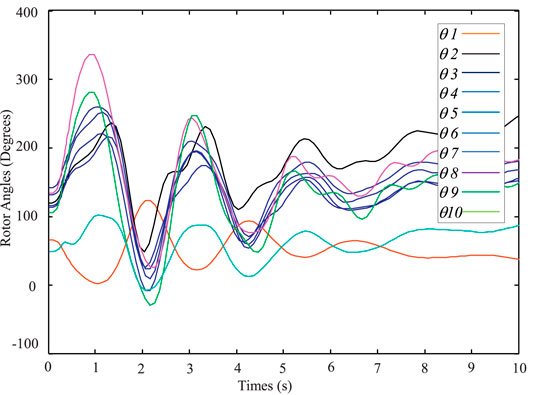
FIGURE 6. Unstable case from PSAT.

FIGURE 7

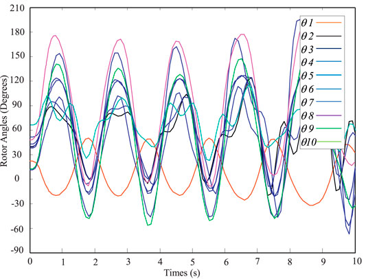
FIGURE 7. Stable case from PSAT.

FIGURE 8

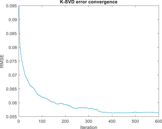
FIGURE 8. Stable dataset K-SVD convergence.

FIGURE 9

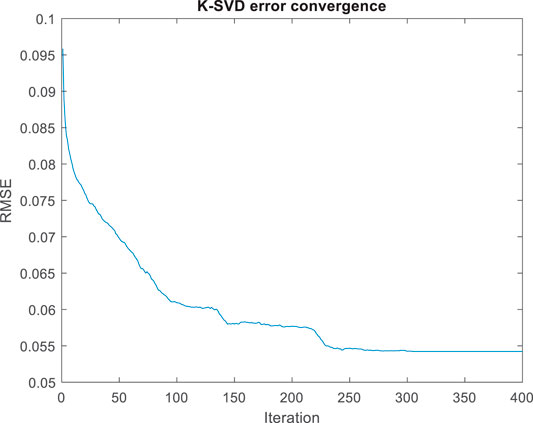
FIGURE 9. Unstable dataset K-SVD convergence.

TABLE 5

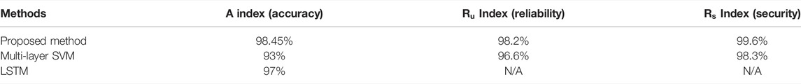
TABLE 5. Comparison of the TSA results.

5.4 Performance Comparison Under Noise Environment

In practical applications and real industrial environments, any uncertain scenarios such as noise are inevitable in PMU measurement. The aforementioned simulation was only implemented under the ideal conditions without any noise. In order to investigate the diagnostic ability of the proposed approach under noise environments, different levels of white Gaussian noise are artificially added to the model with different signal-to-noise ratios (SNRs). This experiment is conducted in the condition of a 50% transmission line length fault location. The main contribution of the proposed approach is applying the sparse dictionary learning method to solve the stability of the power system. Therefore, in terms of this principle, the noises are not considered during the PMU measurement. Instead of that, all the SNRs are added to the K-SVD algorithm in the sparse representation process to obtain the optimal dictionaries under the noise environment. The diagnostic result is given in Table 6. The intensive noise condition is under $SNR=-2$, where the classification accuracy is around 78%. After that, with a continuously increased SNR ratio, the accuracy rates present an obvious upward trend correspondingly. From the results, it is clear to find that the proposed method retains a relatively high classification accuracy rate with a variety of SNRs.

TABLE 6

TABLE 6. Performance with difference degrees of noise.

6 Conclusion

An advanced artificial intelligence method using sparse dictionary learning is presented in this study to improve the transient stability of the power system in classification accuracy, reliability, and secure operation. The New-England 39-bus system is adopted to validate the proposed approach. By comparing the experimental results with the case studies and the discussions presented in the study, the following conclusions can be drawn:

• Timely feedback and adaptation are major evaluation factors in power systems. Implementation of the sparse dictionary learning method is time-saving and straightforward since the proposed method eliminates the feature selection process. In addition, the proposed approach could apply to a variety of models as we only need the sparse dictionary to find the optimal sparse representation of the input data.

• Not only the stability but also the reliability and security are the top priority for running a system. Compared with other AI methods, the proposed method improves 2–6% of the classification accuracy and reduces approximately 1.5 percent of the false alarms. Furthermore, the difference in the accuracy rate after the noises adding to the system is acceptable, which proves the robustness of the proposed method under a noise environment.

• The proposed method could help the system operator by providing a good decision-making tool, which improves the stability of the system operation and decreases the possibility of blackouts happening.

Data Availability Statement

The original contributions presented in the study are included in the article/Supplementary Material; further inquiries can be directed to the corresponding author.

Author Contributions

QW: Conceptualization, methodology, software, and writing the original draft. CP: Supervised, reviewed, and revised the manuscript. CQ: Modeled, reviewed, and revised the manuscript. All authors have read and agreed to the final version of the manuscript.

Conflict of Interest

Author CQ was employed by the company Burns & McDonnell Engineering Co., Inc.

The remaining authors declare that the research was conducted in the absence of any commercial or financial relationships that could be construed as a potential conflict of interest.

Publisher’s Note

All claims expressed in this article are solely those of the authors and do not necessarily represent those of their affiliated organizations, or those of the publisher, the editors and the reviewers. Any product that may be evaluated in this article, or claim that may be made by its manufacturer, is not guaranteed or endorsed by the publisher.

References

Aharon, M., Elad, M., and Bruckstein, A. (2006). $rm K$-SVD: An Algorithm for Designing Overcomplete Dictionaries for Sparse Representation. IEEE Trans. Signal Process. 54, 4311–4322. doi:10.1109/TSP.2006.881199

CrossRef Full Text | Google Scholar

Akhavan, S., Baghestani, F., Kazemi, P., Karami, A., and Soltanian-Zadeh, H. (2022). Dictionary Learning for Sparse Representation of Signals with Hidden Markov Model Dependency. Digit. Signal Process. 123 (2022), 103420. doi:10.1016/j.dsp.2022.103420

CrossRef Full Text | Google Scholar

Bahbah, A. G., and Girgis, A. A. (2004). New Method for Generators' Angles and Angular Velocities Prediction for Transient Stability Assessment of Multimachine Power Systems Using Recurrent Artificial Neural Network. IEEE Trans. Power Syst. 19, 1015–1022. doi:10.1109/TPWRS.2004.826765

CrossRef Full Text | Google Scholar

Cai, D., Li, K., He, S., Li, Y., and Luo, Y. (2019). A Highly Accurate and Fast Power Quality Disturbances Classification Based on Dictionary Learning Sparse Decomposition. Trans. Inst. Meas. Control 41 (1), 145–155. doi:10.1177/0142331218758886

CrossRef Full Text | Google Scholar

Candes, E. J., and Donogo, D. L. (2000). Curvelets - A Surprisingly Effective Nonadaptive Representation for Objects with Edges. Curves and Surfaces.

Google Scholar

Chan, K. W., Cheung, C. H., and Su, H. T. (2002). “Time Domain Simulation Based Transient Stability Assessment and Control,” in Proceedings International Conference on Power System Technology, Kunming, China, 13-17 Oct. 2002 (IEEE), 1578–1582. doi:10.1109/ICPST.2002.1067798

CrossRef Full Text | Google Scholar

Chen, S., Billings, S. A., and Luo, W. (1989). Orthogonal Least Squares Methods and Their Application to Non-linear System Identification. Int. J. Control 50 (5), 1873–1896. doi:10.1080/00207178908953472

CrossRef Full Text | Google Scholar

Chen, S. S., Donoho, D. L., and Saunders, M. A. (2001). Atomic Decomposition by Basis Pursuit. SIAM Rev. 43 (1), 129–159. doi:10.1137/s003614450037906x

CrossRef Full Text | Google Scholar

Do, M. N., and Vetterli, M. (2005). The Contourlet Transform: An Efficient Directional Multiresolution Image Representation. IEEE Trans. Image Process. 14, 2091–2106. doi:10.1109/TIP.2005.859376

PubMed Abstract | CrossRef Full Text | Google Scholar

Donoho, D. L., Elad, M., and Temlyakov, V. N. (2006). Stable Recovery of Sparse Overcomplete Representations in the Presence of Noise. IEEE Trans. Inf. Theory 52, 6–18. doi:10.1109/tit.2005.860430

CrossRef Full Text | Google Scholar

Elad, M., and Aharon, M. (2006). Image Denoising via Sparse and Redundant Representations over Learned Dictionaries. IEEE Trans. Image Process. 15 (12), 3736–3745. doi:10.1109/tip.2006.881969

PubMed Abstract | CrossRef Full Text | Google Scholar

Gomez, F. R., Rajapakse, A. D., Annakkage, U. D., and Fernando, I. T. (2011). Support Vector Machine-Based Algorithm for Post-Fault Transient Stability Status Prediction Using Synchronized Measurements. IEEE Trans. Power Syst. 26 (3), 1474–1483. doi:10.1109/tpwrs.2010.2082575

CrossRef Full Text | Google Scholar

Gupta, A., Gurrala, G., and Sastry, P. S. (2017). “Instability Prediction in Power Systems Using Recurrent Neural Networks,” in Proceedings of the 26th International Joint Conference on Artificial Intelligence (IJCAI'17), Melbourne, Australia, Augest 19-25, 2017 (AAAI Press), 1795–1801. doi:10.24963/ijcai.2017/249

CrossRef Full Text | Google Scholar

Hu, W., Lu, Z., Wu, S., Zhang, W., Dong, Y., Yu, R., et al. (2018). Real-time Transient Stability Assessment in Power System Based on Improved SVM. J. Mod. Power Syst. Clean. Energy 7, 26–37. doi:10.1007/s40565-018-0453-x

CrossRef Full Text | Google Scholar

Han, T., Jiang, D., Sun, Y., Wang, N., and Yang, Y. (2018). Intelligent Fault Diagnosis Method for Rotating Machinery via Dictionary Learning and Sparse Representation-Based Classification. Measurement 118, 181–193. doi:10.1016/j.measurement.2018.01.036

CrossRef Full Text | Google Scholar

Hochreiter, S., and Schmidhuber, J. (1997). Long Short-Term Memory. Neural Comput. 9 (8), 1735–1780. doi:10.1162/neco.1997.9.8.1735

PubMed Abstract | CrossRef Full Text | Google Scholar

Huang, T., and Wang, J. (2019). A Practical Method of Transient Stability Analysis of Stochastic Power Systems Based on EEAC. Int. J. Electr. Power & Energy Syst. 107, 167–176. doi:10.1016/j.ijepes.2018.11.011

CrossRef Full Text | Google Scholar

Kakimoto, N., Ohnogi, Y., Matsuda, H., and Shibuya, H. (1984). Transient Stability Analysis of Large-Scale Power System by Lyapunov's Direct Method. IEEE Power Eng. Rev. 4 (1), 41. doi:10.1109/mper.1984.5525444

CrossRef Full Text | Google Scholar

Kundur, P., Paserba, J., Ajjarapu, V., Andersson, C., Bose, A., Canizares, C., et al. (2004). Definition and Classification of Power System Stability. IEEE Trans. Power Syst. 19 (3), 1387–1401. doi:10.1109/TPWRS.2004.825981

CrossRef Full Text | Google Scholar

Lachiheb, O., Gouider, M. S., and Said, L. B. (2015). “An Improved MapReduce Design of Kmeans with Iteration Reducing for Clustering Stock Exchange Very Large Datasets,” in Proceedings of the 2015 11th International Conference on Semantics, Knowledge and Grids (SKG), Beijing, China, 19–21 August 2015 (IEEE), 252–255. doi:10.1109/skg.2015.24

CrossRef Full Text | Google Scholar

Li, Y., Wang, R., and Yang, Z. (2022). Optimal Scheduling of Isolated Microgrids Using Automated Reinforcement Learning-Based Multi-Period Forecasting. IEEE Trans. Sustain. Energy 13 (1), 159–169. doi:10.1109/TSTE.2021.3105529

CrossRef Full Text | Google Scholar

Li, Y., and Yang, Z. (2017). Application of EOS-ELM with Binary Jaya-Based Feature Selection to Real-Time Transient Stability Assessment Using PMU Data. IEEE Access 5, 23092–23101. doi:10.1109/ACCESS.2017.2765626

CrossRef Full Text | Google Scholar

Liu, C., Jiang, D., and Yang, W. (2014). Global Geometric Similarity Scheme for Feature Selection in Fault Diagnosis. Expert Syst. Appl. 41, 3585–3595. doi:10.1016/j.eswa.2013.11.037

CrossRef Full Text | Google Scholar

Mairal, J., Elad, M., and Sapiro, G. (2008). Sparse Representation for Color Image Restoration. IEEE Trans. Image Process. 17, 53–69. doi:10.1109/TIP.2007.911828

PubMed Abstract | CrossRef Full Text | Google Scholar

Mallat, S. (1999). A Wavelet Tour of Signal Processing. Elsevier Science.

Google Scholar

Mallat, S. G., and Zhifeng Zhang, Z. (1993). Matching Pursuits with Time-Frequency Dictionaries. IEEE Trans. Signal Process. 41 (12), 3397–3415. doi:10.1109/78.258082

CrossRef Full Text | Google Scholar

Milano, F. (2005). An Open Source Power System Analysis Toolbox. IEEE Trans. Power Syst. 20 (3), 1199–1206. doi:10.1109/TPWRS.2005.851911

CrossRef Full Text | Google Scholar

Padiyar, K. R. (1990). Energy Function Analysis for Power System Stability. Electr. Mach. Power Syst. 18 (2), 209–210. doi:10.1080/07313569008909464

CrossRef Full Text | Google Scholar

Protter, M., and Elad, M. (2008). Image Sequence Denoising via Sparse and Redundant Representations. IEEE Trans. Image Process. 18, 27–35. doi:10.1109/TIP.2008.2008065

PubMed Abstract | CrossRef Full Text | Google Scholar

Ren, L., Xiao, W. S. Y., Jiang, S., and Xiao, Y. (2016). Fault Diagnosis Using a Joint Model Based on Sparse Representation and SVM. IEEE Trans. Instrum. Meas. 65, 2313–2320. doi:10.1109/tim.2016.2575318

CrossRef Full Text | Google Scholar

Rubinstein, R., Faktor, T., and Elad, M. (2012). “K-SVD Dictionary Learning for the Analysis Sparse Model. Kyoto, Japan: ICASSP 2012.

Google Scholar

Rubinstein, R., Zibulevsky, M., and Elad, M. (2008). Efficient Implementation of the K-SVD Algorithm Using Batch Orthogonal Matching Pursuit. Technical Report - CS Technion.

Google Scholar

Scala, M., Sbrizzai, R., Torelli, F., and Scarpellini, P. (1998). A Tracking Time Domain Simulator for Real-Time Transient Stability Analysis. IEEE Trans. Power Syst. 13 (3), 992–998. doi:10.1109/59.709088

CrossRef Full Text | Google Scholar

Stankovic, L., Sejdi´c, E., Stankovi´c, S., Dakovi´c, M., and Orovi´c, I. (2019). A Tutorial on Sparse Signal Reconstruction and its Applications in Signal Processing. Circuits. Syst. Signal Process. 38, 1206–1263. doi:10.1007/s00034-018-0909-2

CrossRef Full Text | Google Scholar

Vittal, V., Zhou, E.-Z., Hwang, C., and Fouad, A. A. (1989). Derivation of Stability Limits Using Analytical Sensitivity of the Transient Energy Margin. IEEE Power Eng. Rev. 9 (11), 33–34. doi:10.1109/MPER.1989.4310369

CrossRef Full Text | Google Scholar

Wang, B., Fang, B., Wang, Y., Liu, H., and Liu, Y. (2016). Power System Transient Stability Assessment Based on Big Data and the Core Vector Machine. IEEE Trans. Smart Grid 7 (5), 2561–2570. doi:10.1109/tsg.2016.2549063

CrossRef Full Text | Google Scholar

Wang, Q., Pang, C., and Alnami, H. (2021a). “Transient Stability Assessment of a Power System Using Multi-Layer SVM Method,” in 2021 IEEE Texas Power and Energy Conference (TPEC), College Station, TX, USA, 2-5 Feb. 2021 (IEEE), 1–5. doi:10.1109/TPEC51183.2021.9384918

CrossRef Full Text | Google Scholar

Wang, Q., Pang, C., and Alnami, H. (2021b). “Transient Stability Prediction Based on Long Short-Term Memory Network,” in 2021 North American Power Symposium (NAPS), College Station, TX, USA, 14-16 Nov. 2021 (IEEE), 01–06. doi:10.1109/NAPS52732.2021.9654462

CrossRef Full Text | Google Scholar

Xiang, L., Wang, X-H., and Wang, J. (2007). Feature Selection for SVM Based Transient Stability Classification[J]. Relay. 35 (9), 17–21.

Google Scholar

Xue, Y., Van Custem, T., and Ribbens-Pavella, M. (1989). Extended Equal Area Criterion Justifications, Generalizations, Applications. IEEE Trans. Power Syst. 4 (1), 44–52. doi:10.1109/59.32456

CrossRef Full Text | Google Scholar

You, D., Wang, K., Ye, L., Wu, J., and Huang, R. (2013). Transient Stability Assessment of Power System Using Support Vector Machine with Generator Combinatorial Trajectories Inputs. Int. J. Electr. Power & Energy Syst. 44, 318–325. doi:10.1016/j.ijepes.2012.07.057

CrossRef Full Text | Google Scholar

Zhang, S., Zhu, Z., and Li, Y. (2021). A Critical Review of Data-Driven Transient Stability Assessment of Power Systems: Principles, Prospects and Challenges. Energies 1421, 7238. doi:10.3390/en14217238

CrossRef Full Text | Google Scholar