 Falah Alobaid
 Alexander Kuhn1
 Nhut M Nguyen
- 1Technical University of Darmstadt, Institute for Energy Systems and Technology, Darmstadt, Germany
- 2Department of Chemical Engineering, Can Tho University, Can Tho, Vietnam
This study presents a comprehensive dynamic process simulation model of a 1 MWth circulating fluidized bed test facility applied for lignite and refuse-derived fuel co-combustion. The developed dynamic process simulation model describes the circulating fluidized bed riser and the supplying system with a high level of detail considering heat transfer, gas-solid interaction, combustion, and fluid dynamics. The model was first tuned at two steady-state operation points and was then validated by the measured data from a long-term test campaign of the 1 MWth circulating fluidized bed test facility at various loads (60%–80% to 100%). During the load changes, the simulated pressure and temperature profiles along the combustor as well as the flue gas concentrations agree very well with the measurement data. Finally, increasing the proportion of waste-derived fuel in the co-combustion process was investigated to evaluate the flexibility of its use in power generation to further reduce CO2 emissions.
1 Introduction
Climate change is one of the greatest global challenges facing society in the 21st century, actively promoting measures for a flexible and low-carbon energy economy. Here, the introduction of carbon capture technologies and the use of renewable energy sources in power generation, including the electrification of the heating and transport sectors, are of great relevance. However, the increase in the share of renewables in the electricity market points to a crucial drawback, namely their intermittent power generation. Wind power plants, as an example, cannot operate when the wind is too weak or too strong, while solar power plants are in action when the Sun is shining. A reliable source of electricity, e.g., conventional thermal plants or energy storage systems are required to achieve a balance between current electricity supply and demand. An important requirement for a reliable source of electricity is its output being dynamically controllable to compensate for the feed-in fluctuations from renewable energy sources. Refuse-derived fuel (RDF) can contribute to the promotion of renewable energy. It is a substitute fuel made from waste with high calorific value, which is also well suited for environmentally friendly combustion.
A fluidized bed system is a promising technology for the combustion of refuse-derived fuels, as it has very good combustion characteristics. The fluidized bed combustion is characterised by slight temperature gradients, strong mixing and heat transfer capabilities of gas and solids, and high flexibility for solid fuels with a wide range of particle size distribution and form. Additionally, fluidized bed combustors offer high combustion efficiency as well as lower SO2 and NOx emissions due to the lower combustion temperature compared to conventional industrial-scale firing systems. Based on the fluidization velocity and solid properties, a fluidized bed system can be classified into fixed bed, bubbling fluidized bed (BFB), and circulating fluidized bed (CFB) (Kunii et al., 1991). It is noted that recent focus has been done on CFB boilers due to their high combustion efficiency, operational flexibility, the flexibility of solid fuels, and electricity generation at industrial scales up to 660 MWel (Hotta et al., 2010).
In addition to experimental studies, simulations can provide a sufficient approach for evaluating global and local variables of the flow, as well as reproducing the behaviour and phenomena occurring in the process, which in turn can predict and optimise the performance of the system with rapid and cost-effective measures. However, a reliable simulation also has an important challenge, namely the separation of scales, which vary from micro-scale to macro-scale. The large-scale flow structures occur at the reactor scale (order of meters), while micro-scale (from micrometres to millimetres) is the fundamentals of gas and solid flows (gas-solids and particle-particle interactions). Currently, two different approaches are usually applied for the simulation of fluidized bed systems, i.e., computational fluid dynamics (CFD) and process simulation. The CFD approach is often used to simulate single components for visualisation of the flow patterns of the gas/solid path. This approach is relatively accurate but computationally expensive (Kumar et al., 2018). While real-time CFD simulations require significant advances in the accuracy, performance, and efficiency of numerical models, future developments may usher in a new virtual reality era for fluidized beds, using interactive simulations in place of stepwise experimental scale-up studies and costly empirical trial-and-error methods (Alobaid et al., 2021). The process simulation is used to model the entire process system including main unit operations, the gas/solids and water/steam paths, and other supporting units. A process simulation simplifies the computational domain to one-dimensional using empirical correlations for the micro-scale flow structures. However, the experimental data have shown that the flow structure in the fluidized bed is radially unevenly distributed, with higher bed void, higher flow velocity, and higher particle velocity in the central region of the bed and with lower values of the previously mentioned variables in the region close to the wall. Considering these flow characteristics, a core-annulus model has been proposed recently, since it is suitable for describing the flow structure in the fluidized bed. The model assumes two homogeneous flow regions (core and annulus) in the radial direction of the bed and uses the differences between them to describe the radially non-uniform flow structure in the fluidized bed. While this type of model does not give the exact radial flow structure, it is a practical and very useful way to describe the flow structure while waiting for more accurate CFD modelling to be used.
Initially, the process simulation was used to model steady-state processes, which perform a mass, and energy balance of a process independent of time. A large number of steady-state process simulations of the CFB boilers have been published. Guoli et al. (Tang et al., 2019) developed a mathematical model to simulate a 660 MWel ultra-supercritical CFB boiler using low-grade fuels. The results show good flow distribution and small temperature deviation in the evaporator system. Wu et al. (Wu et al., 2018) presented a core-annulus model of a 600 MWel supercritical circulating fluidized bed boiler. The results show that the model can reproduce the characteristics of the CFB quite well. Similar studies on supercritical circulating fluidized bed boilers with a capacity of 600 MWel were also carried out by Wang et al. (Wang et al., 2016) and Pan et al. (Pan et al., 2012). The authors claimed that the heat transfer performance and low flow resistance of the water wall design are applicable and that supercritical CFB boilers have become an important option for coal-fired power plants. Yang et al. (Yang et al., 2005) developed a 1D model of a circulating fluidized bed boiler with a capacity of 135 MWel to predict the ash formation, attrition and size reduction, residence time, and segregation. The model was not validated against the measured data. Wang et al. (Wang et al., 1999) presented a mathematical model for a 12 MW CFB boiler. Test results were used for model verification, showing good agreement.
In contrast to steady-state modelling, fewer publications have been found regarding dynamic process simulation of the CFBs. Dynamic simulation, an extension of steady-state process simulation with time-dependence, offers an essential tool for the design of energy conversion, prediction of the transient behaviour of the combustion chambers, and process configurations under changing conditions (Alobaid et al., 2017; Castilla et al., 2021). A dynamic simulation model of a 750 MWel coal-fired power plant has been developed to evaluate the operation flexibility (Starkloff et al., 2015). The simulation investigated the water steam flow and the heat transfer from the gas side to the water-steam side and the control scheme. Lappalainen et al. (Lappalainen et al., 2014) developed a dynamic simulation of a 300 MWel oxy-CFB boiler in APROS software including the gas-solid interaction, the water-steam side, and the turbines island. It should be noted that very few dynamic models were validated against the measured data in the literature. A dynamic model has been developed for the combustion of Tuncbilek lignite in a CFB combustion chamber (Gungor and Eskin, 2007; Gungor, 2009). The process model shows a good agreement with measured results obtained from the 50 kW Gazi University heat power pilot-scale unit. Luo et al. (Luo et al., 2015) developed an oxy-fuel combustion process model based on a 3 MWth test facility under steady-state and dynamic conditions using Aspen Plus and Aspen Plus Dynamics. The steady-state model was compared with experimental results based on mass and energy balance, while dynamic features of the control actuators and the responses of heat transfer and fluid flow processes to reproduce the dynamic responses of the system characterised the dynamic model. The dynamic simulation results match the measured data well. A core-annulus model was proposed to simulate the axial distribution of gas and solid phases in a large-scale CFB boiler (Chen and Xiaolong, 2006). The model is used to describe the radial distributions of solid particles and particle clusters in the system. The simulation temperatures were compared with the measured values in the combustor for a very short time (30 s). Alobaid et al. (Alobaid et al., 2020) developed a dynamic process simulation of a CFB furnace based on the 1-MW test facility with a high level of detail including the CBF riser, the air supply, the flue gas path, the water-cooling system, and the control structures. The numerical results are in good agreement with the measured data at various load cases. The validated model can predict the transient behaviour of the process variables of gas and solids flows during lignite combustion. The model used in the previous study was extended by Peters et al. (Peters et al., 2020) to perform the specific characteristics of a CFB furnace during the dynamic operation of polish lignite. The process simulation model was tuned with the measurement of a steady-state test point and validated with experimental data of the load cycling test.
Due to the limited existing works regarding the dynamic process simulation of circulating fluidized bed boilers during part loads (Alobaid et al., 2020), particularly using alternative fuels (e.g., refuse-derived fuel), this study aims to develop a dynamic model of a fluidized bed co-combustion of lignite and RDF to investigate the flexibility of compensation for fluctuating power generation, and to increase the proportion of RDF while reducing the proportion of lignite to further reduce CO2 emissions. For this purpose, a 1.5D dynamic process simulation model of the 1MWth circulating fluidized bed test facility at the Technical University of Darmstadt is developed in APROS, which considers the heat transfer, gas-solid interaction, and combustion. The developed model was validated against steady-state and dynamic experimental results, and subsequently, the effects of increasing the proportion of RDF were investigated. The novelty and the objectives of this study are presented as follows.
1. A dynamic process simulation model for the co-combustion of lignite and RDF was developed for the first time to predict the transient behaviour of CFB furnaces during load change.
2. The model was validated at various steady-state and dynamic operating conditions, including an increasing load from 60% to 80% and 100%, followed by a load decrease from 100% to 80% and 60% as well as a load increase from 60% to 100%. The simulated pressure, temperature and flue gas contents show good agreement with the measured results from a long-term test campaign.
3. The increasing share of RDF in the co-combustion was investigated to evaluate the flexibility of using pure RDF for power generation to further reduce CO2 emissions.
This paper is organised as follows. Section 2 presents the configuration of the 1 MWth test system. In Section 3, the modelling approach and the model structure are described. Section 4 demonstrates the developed dynamic simulation model and all assumptions used as well as the simulation results and discussions. The main remarks and conclusions obtained from the study are highlighted in Section 5.
2 The 1 MWth circulating fluidized bed test system
The experimental test facility mainly comprises a riser and a solid recirculation system, illustrated in Figure 1. The riser has an inner diameter of 0.59 m and a total height of 8.6 m. The insulation was developed according to industrial standards with a thickness of 0.355 m. The system configuration is shown in Table 1. The main components of the experimental facility are the air-supply system (primary air, secondary air, and burner air), the reactor with its solid circulation (cyclone and loop seal) the cooling system, and flue gas paths (heat exchanger, bag filter, and induced-draft fan).
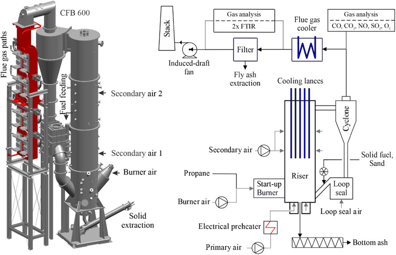
FIGURE 1. 1 MWth fluidized bed test facility and its flow diagram.
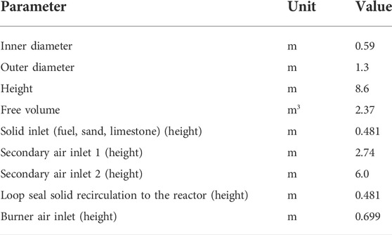
TABLE 1. Design parameters of the combustor.
The primary air is electrically preheated to 300°C before injecting via the 30 nozzles grid at the bottom of the riser, while the secondary air is injected into the reactor at different heights (2.74 m and 6.0 m) and the burner air enters at a height of 0.7 m at 25°C. The solid materials including fuels, sand, and limestone are fed into the riser through the return leg of the loop seal and separated from the flue gas by the cyclone after leaving the riser. Bed materials can be discharged at the bottom through a cooled screw conveyor to keep the solid inventory in the riser within a desired range. To control the temperature in the riser, the cooling system with five cooling lances can be immersed vertically to remove the excess heat from the riser. The cooling system operates under a pressure of 8–16 bar. After leaving the cyclone, the hot flue gas flows through the flue gas paths, which are installed convective tube bundle heat exchangers to cool down before passing a fabric filter to remove fly ash. Finally, the cooled flue gas exits the system at a temperature of 130–150°C.
3 Modelling approach
The process simulation in this study was carried out in APROS software, which is a multifunctional simulation program developed by Fortum and the Technical Research Centre of Finland (VTT) (Haenninen, 2009; Lappalainen et al., 2014; Lappalainen et al., 2017; Hiidenkari et al., 2019; Alobaid et al., 2020). The program can simulate thermal combustion power plants, energy, and industrial processes as well as safety analysis by using specialised component libraries for the process, automation, and electrical systems. The simulation is performed by selecting the required process components (valve, pump, fan, heat exchanger, etc.) from the component libraries together with connections for materials, energy, or heat to build a model of an existing process and/or a new system for research. To customize the simulation model, all required design parameters (configuration of the heat exchanger, the characteristic curve of the pump, etc.) can be inserted into process components, which are linked by electrical and automation signals for controlling purposes. In the recent literature, APROS models have been usually used to simulate thermal power plants. Most studies performed validation of the numerical results based on the experimental measurement for the accuracy and readability of the developed models including combined-cycle power plants (Alobaid et al., 2008; Mertens et al., 2016a; Mertens et al., 2016b; Angerer et al., 2017; Bany Ata et al., 2020), coal-fired power plants (Schuhbauer et al., 2014; Starkloff et al., 2015; Starkloff et al., 2016; Hentschel et al., 2017; Peters et al., 2020), circulating fluidized bed (Lappalainen et al., 2014; Mikkonen et al., 2015), concentrated solar power plant (Henrion et al., 2013; Al-Maliki et al., 2016a; Al-Maliki et al., 2016b), nuclear power plant (Arkoma et al., 2015), municipal waste incinerator (Alobaid et al., 2018).
3.1 Model description
The model in this paper describes the co-combustion of coal and RDF materials developed in APROS software based on the piping and instrumentation diagrams of the 1 MWth circulating fluidized bed system, located at the Technical University of Darmstadt. The model consists of five different sections, including the reactor with material circulation, the insulation, the ramps used for data input, the fluid, and solid feeds and removals, and the cooling system. Figure 2 shows an overview of the structure of the model. The standard process components in the APROS libraries are available for the simulation, such as pump, fan, pipe, heat exchanger, etc., while in-house calculation structures are implemented into the model for the missing components (e.g., fittings, fabric filter, and air heater, etc.). The model was tuned at two steady-state load cases, i.e., 60% and 100%, which correspond to the lowest load and the highest load case of the dynamic course in the experimental data. The simulation results were compared with the measurement data. In the dynamic simulation, the load increases from 60% to 80% and then to 100%, followed by a reduction in a dynamic load from 100% to 80% and then to 60%, before increasing again to 100% were simulated. At each simulation point, the temperature and pressure profiles along the reactor as well as the flue gas contents (e.g., CO2, O2, and H2O) were compared with the experimental data. Additionally, the transient behaviour of the bed temperature and the flue gas temperature at the outlet of the cyclone were plotted and validated against the test facility. The different sections in the model are explained in the following sub-sections.
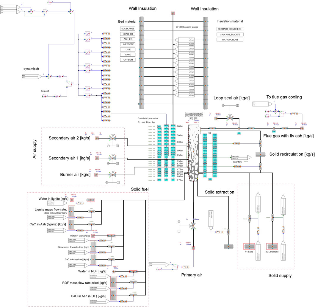
FIGURE 2. Overview of the dynamic model.
3.2 Fluidized bed combustor
The circulating fluidized bed (CFB 600) furnace, shown in Figure 2, includes a riser, and a recirculation system for solids (i.e., a cyclone, a standpipe, and a loop seal), and water-cooled lances. The riser has a total height of about 8.6 m and a free volume of 2.368 m3, which is divided into 20 calculation nodes at different heights. The distance between the two nodes ranges from 0.2 m to 0.75 m. The gas fraction is only calculated vertically and the solid with the core-annulus approach. In this approach, each node is divided into a central cylinder and an outer annulus, where solid particles can rise in the core area, while it can fall at the edge of the riser. However, the gases only flow up through the riser. In the simulation, the chemical reactions that take place in the combustion process are presented as follows (Alobaid et al., 2020):
The pyrolytic components released from the pyrolysis reaction (1) are proportional to the defined concentrations by the user. The reaction rate of char combustion rchar assumes that the boundary layer diffusion controls the chemical reactions (Ylijoki et al., 2005):
Where pO2 is the average partial pressure of oxygen, pO2,sur stands for the partial pressure of oxygen at the surface of char particles, dchar represents the diameter of char particles, and Tgas is the gas temperature. The parameter ψ has the value of two for the reaction (2), and the value of unity for the reaction (3), while D is a parameter that is a function of the gas temperature. The reaction rate of the volatiles (reaction (4) to (8)) strongly depends on volatile components, oxygen content in the combustor, and the contact of oxygen and volatiles (the degree of turbulence). The reaction rate of these reactions is proposed by Magnussen (Magnussen and Hjertager, 1977) as follows.
Here, τtur represents the time scale of turbulent mixing, Cvol and Coxy are the concentration of volatile species and oxygen, respectively. n and m are obtained from the fuel CnHm, and Vnod is the volume of the calculation node.
The temperature in the fluidized bed reactor is controlled using five water-cooled lances that can be moved vertically. The mass flow rate of water is kept constant, the temperature can be controlled by changing the immersed depth of these lances in the riser. In the experimental investigations, however, the depths of these lances were fixed (e.g., the immersed depth of two lances was 4.5 m, and the other three were kept at the immersed depth of 6.5 m). The positions of these water-cooled lances directly influence the heat exchange and the temperature in the riser. The lances are modelled with the calculation nodes in the riser (from node 6 to node 20).
3.2.1 Insulation
The walls of the riser are refractory lined, comprising the innermost layer of refractory concrete, which is covered with a layer of calcium silicate and other thermal insulation. In the simulation, the thermal properties of the insulating material are considered as a function of temperature which is used to calculate the heat loss to the atmosphere and the heat storage/release of refractory lining walls during load changes. The calculation of the heat transfer coefficients is based on empirical models in APROS and the material properties of the refractory lining walls.
3.2.2 Air supply
The combustion air (primary, secondary, and burner air) is injected into the reactor at different heights. An air-fuel ratio (excess air factor) of 1.2 is used, which is required for optimum combustion and emission in the fluidized bed combustion. This ratio varies slightly with different load changes, as additional primary air should be supplied to achieve sufficient fluidization and to ensure solid entrainment (circulating fluidized bed).
The primary air is preheated to approximately 300 °C and considered as a constant value during simulation before injecting to fluidize the solid materials in the riser. To reach the required mass flow rate or volumetric flow rate, a primary air fan is used to pressurize atmospheric air, which is controlled by a PI controller to adjust the speed of the primary air fan through a frequency converter. The pressure after the fan is determined by the mass flow rate and the performance characteristics curve of the primary air fan. The other streams are injected at an ambient temperature of 25°C. The pressure of all air streams supply at 1.5 bar. The loop seal air is supplied without being preheated. Due to contact with hot recirculated solid materials during passing the standpipe and the cyclone, the loop seal air increases from ambient temperature to 300°C. At the outlet of the cyclone, the loop seal air is finally mixed with the hot flue gas from the combustor. All control structures and process components in the model are the standard process components of the APROS libraries, except for the preheater. The ramps of the primary air, secondary air, and burner air were adjusted manually. The ramps of the recirculation air were added during this elaboration. The fluid air is defined with a nitrogen mass fraction of 77% and an oxygen mass fraction of 23%.
3.2.3 Solid feeding
Two different types of solid materials are fed into the riser, i.e., solid fuels and sand. The solid fuels used in the experimental investigations are lignite, straw pellets, and refuse-derived fuel (RDF). However, this simulation is mainly carried out with the co-combustion of lignite and RDF. Lignite is non-dried ground coal from western Germany and its moisture content is within the normal range for non-dried, low calorific coal. The RDF material is mainly composed of flat and light pieces such as films, paper, or textile materials. The properties of the solid fuels are shown in Table 2.
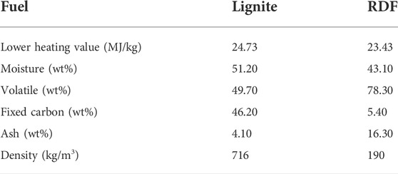
TABLE 2. The properties of the solid fuels.
In the simulation, the solid materials are fed into the riser at the height of 0.481 m. It is noted that the water and calcium oxide in the solid fuel are supplied separately to the riser, preventing numerical instability according to the software user. This can be achieved by using a pipe and a point for the water inlet as well as a particle transmitter for the calcium oxide inlet. Two inlets were connected to the riser at the height of 0.481 m, in the same position with solid feeding. The respective control data of the mass flow rates are determined by the value of the ramps and the fuel properties measured in the experiment. The amount of the water inlet is a function of the moisture content in each raw solid fuel, the fraction of solid fuel used, and the total mass flow rate of the solid fuels. The calcium oxide mass flow rate is also calculated by using a similar approach with consideration of the mass fraction of the calcium oxide in the ash. The moisture is supplied to the riser as a liquid phase at 25°C and a pressure of about 1.2 bar. The calcium oxide is fed into the riser at 25°C. Additionally, the sand enters the riser as bed materials at different mass flow rates depending on the load. The solid and gas mass flow rates are in Table 4.
To keep the mass inventory (total mass of solid particles) in the riser constant despite a constant supply of solid fuels, a portion of the bed material is discharged at the bottom of the riser, including ash, sand, and unreacted fuels. The constant mass inventory of the bed is to maintain the desired fluidization, combustion, and heat transfer conditions (Alobaid et al., 2020). To achieve that, a solid balance in the riser should be considered. In the model, the bottom of the riser relates to a heat structure and a particle transmitter via the solid extraction line (see Figure 1). It should be noted that the simulation cannot reproduce the experimental conditions identically. In the experimental investigations, the pressure drop through the bed is measured. If the pressure drop is above a specific limit, a certain amount of the solid will be extracted from the riser, while the simulation runs continuous removal. The composition of the removed solid material corresponds to the material composition at the lowest simulation area. Two types of solid materials enter the riser, i.e., sand and solid fuels. In the combustion of solid fuels, the volatile and char will be oxidized, while inert materials, e.g., ash and sand, are accounted for the solid balance. The mass flow rate of the solid extracted from the riser is determined by the sum of these solids (sand, ash, etc.) to maintain a constant bed inventory in the riser. To achieve this, the actual mass inventory is compared with the predefined setpoint (an inventory of 130 kg) to determine the extracted solid mass flow rate. In the case of the actual mass inventory being smaller than the setpoint, sand will be fed into the riser. Additionally, the fraction of the extracted solid can be defined based on the solid composition in the bottom node.
3.3 Flue gas path
The exhaust gas from the top of the combustor at a temperature of about 720°C flows through heat exchangers, venture nozzle, and fabric filter to the stack. The heat exchangers, including membrane and convective tube bundle heat exchangers, are used to cool down the gas using water as a cooling medium and are arranged in two vertical rectangular flue gas paths. In the simulation, the free cross-sectional area is applied based on the hydraulic diameter. After leaving the second path, the flue gas flows into a horizontal path where different built-in components are installed, such as venture nozzles and fabric filters. However, equivalent process components are not available in the APROS library. Therefore, these components are simulated based on pressure drop and thermal masses. To push the flue gas to the stack, the constant negative pressure of about 1 mbar in the cyclone is generated by an induced-draft fan. To achieve that, a comparison is made between the actual pressure in the cyclone and the setpoint. A PI controller is used to adjust the speed of the induced-draft fan by changing the frequency converter of the fan. Lastly, the flue gas is released into the atmosphere at a temperature of around 130°C. These components (vertical and horizontal paths, the membrane wall and tube bundle heat exchangers, the induced-draft fan, and all connection pipes) are modelled using APROS library process components and in-house calculation structures with the real specification of the experimental facility. The ambient conditions (temperature and pressure) are defined as boundary conditions for the stack.
3.4 Cooling system
The water-cooling system in the experimental facility consists of two main process systems, namely CFB600 water-cooling lanes and a flue gas cooling system. The heat transfer of the cooling lances directly influences the reactor temperature and the combustion; thus, the cooling lances are considered in the simulation. For this purpose, a system of heat transfer pipes and heat exchangers is integrated into the model, which transfers the heat from the individual nodes into the water-bearing pipes. The cooling lances can be immersed in the reactor at a depth of up to 6 m. The simulation of the cooling lance system is carried out without the consideration of a re-cooling process; therefore, the inlet of the cooling water is considered as boundary conditions with a temperature of 110°C and a pressure of about 11 bar corresponding to a flow of 3.96 kg/s. To reach the setpoint, the PI controller can change the speed of the pump via a frequency converter. Additionally, the temperature of the cooling water in the process-cooling lines is considered a critical parameter during control. If the temperature exceeds the maximum specified setpoint (here is 160°C), the control logic in the system will change from the water mass flow rate setpoint to the maximum temperature setpoint of the cooling water, resulting in the adjustment of the speed of the cooling water pump and then the water mass flow rate until the maximum temperature in each process-cooling lance is below the predefined setpoint.
3.5 Measurement system
Various measuring devices were installed at key points in the 1 MWth CFB pilot plant. The measurement data were continuously recorded and stored in the process control system. Some of the measured values were used to evaluate the process, while the remaining measurements were needed to control the material and heat flows and to ensure the operational reliability of the 1 MWth CFB pilot plant. The measurement uncertainty of the directly measured values (e.g., static pressure, temperature, and flue gas concentrations) depends only on the relative uncertainty of the measuring instruments and was given by the relative error (see Table 3). For indirectly measured parameters or calculated values (e.g., volumetric flow, where the pressure difference and temperature are used for calculation), the Gaussian error propagation method was used assuming normally distributed uncertainties.
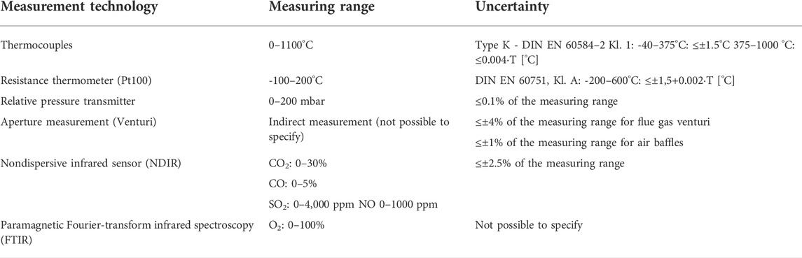
TABLE 3. Measuring range and relative systematic measurement uncertainty.
3.6 Dynamic boundary conditions
The dynamic boundary conditions perform the load changes according to the experimental data. The parameters, such as temperatures, pressures, and air mass flow rates as well as the solid mass flow rates were implemented as a function of time. The dynamic boundary conditions are determined as a load increase from 60% to 80% to 100% and a load decrease from 100% to 80% to 60% and then its increase to 100%, as shown in Figure 3. For the dynamic simulation, it is required to activate the timer of the appropriate load change and then boundary conditions of the unsteady simulation are implemented. The numerical results, e.g., temperature and pressure profiles along the combustor, gas, and solid contents were obtained as text files during simulation runs.
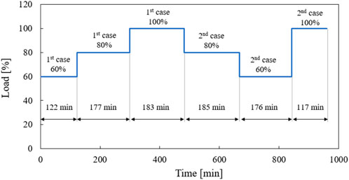
FIGURE 3. The load changes of the dynamic test series.
4 Results
4.1 Model tuning
To tune the simulation model to the experimental conditions, some parameters were determined. The tuning can be divided into four main groups. However, these four groups influence each other and lead to a complicated and time-consuming tuning process with several iterations. The main groups consist of particle velocity in the riser, the pressure curve, the temperature curve, and CO release. Figure 4 shows a flow chart of the tuning process flow. The simulation model is tuned to fit two steady-state cases with the second 60% and 100% load cases, which represent both the lowest and the highest load cases of the dynamic curve in the experimental investigations. The other simulated values are calculated by linear interpolation. The model is iteratively calculated to improve the simulation results for good agreement with the measurement data. The influence of different parameters, variables, and methods on the model performance is evaluated to select the most preferable values and methods. Table 4 shows the boundary conditions at different loads during the measurement test.
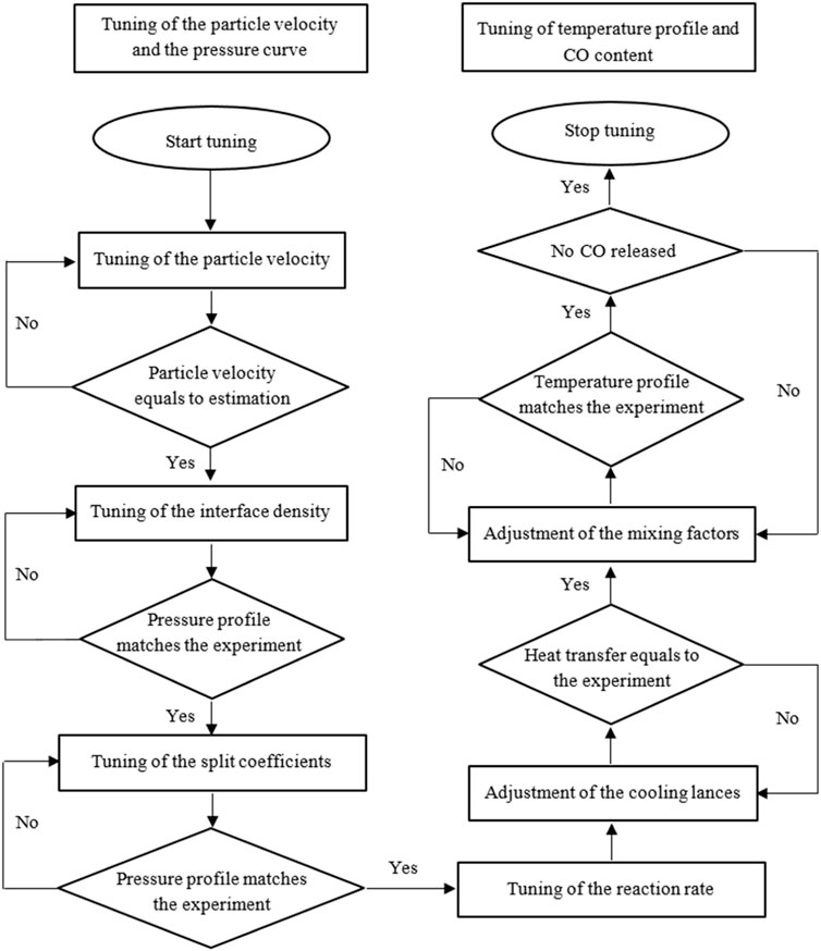
FIGURE 4. Flowchart of the tuning process.
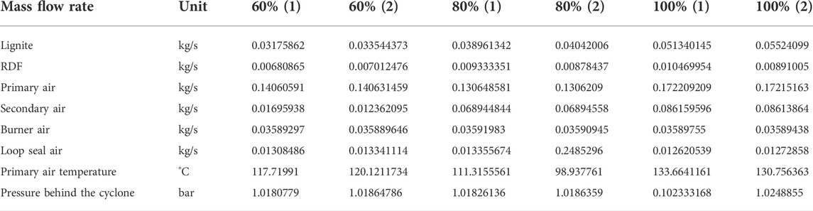
TABLE 4. Boundary conditions at different loads.
4.2 Mixing factors
The mixing of the solid particles with oxygen inside the riser is not ideal. To simulate this behaviour, mixing factors are implemented that control the availability of oxygen for combustion. These factors are implemented by tuned ramps.
The input value of the ramps (RE is, as seen in formula 11, a product of the total air mass flow of the reactor (ML,ges) and the sum of 1 and the fraction of the difference of the coal mass flow setpoint (Mc,soll) and the actual coal mass flow value (Mc,ist) divided by the coal mass flow setpoint (Mc,soll). Variations in the actual coal mass flow rate relative to the setpoint, thus provide an increase or decrease in the mixing factors.
For a more accurate simulation of the combustion process in a fluidized bed reactor, the solid particle velocity must be considered. The velocity consists of two parts due to the core-annulus approach. At the core where fuel and bed particles are entrained by the upflowing air, the velocity is assumed to be positive in the direction of the airflow. The other part is the annulus, in which some of the particles discharged from the bed fall back down the sides of the reactor. According to the definition, the velocity of these particles is negative.
The solid particle velocity in the core is calculated as a function of gas velocity in the core vg,c and terminal velocity vt. The terminal velocity of the particles, vt, is calculated in APROS within the module and can only be influenced by external factors. The solid particle velocity in the core is calculated as follows.
Where αtv is an adjustable factor, and βsv,C represents a constant to compensate for an offset of the velocity.
The gas velocity in the annulus (vg,A) can be adjusted by the factor αgv,A as a function of the gas velocity in the core calculated by APROS. In this work, αgv,A is set to 0.1 which is estimated from empirical values for the fluidized bed reactor.
The particle velocity in the annulus area is calculated as follows.
With αgv,A is a coefficient of terminal velocity in the annulus area, it is set to 1 in this simulation. The particle flow in circulating fluidized bed reactors was investigated experimentally (Daikeler, 2019). The investigation determined the velocity of the solid particles over the cross-section of the reactor. Since sand was used as the main component of the solid particles in the reactor, this was used as a comparative value. Additionally, the interface density is the first parameter for setting the pressure, which defines the density of the fluidized bed. This value mainly affects the lower part of the reactor, so this value is tuned first.
Within the reactor, a permanent exchange of solid particles of the core and ring area takes place. In the process, particles get from the lean zone into the dense zone and vice versa. The number of transferred particles is calculated by APROS itself. A correction of the carryover is only possible via a coefficient. This split coefficient is divided into a global and a local split coefficient. In addition, both the global and the local split coefficients are subdivided into alpha and beta. Alpha is used in the calculation of particle flow from the core area to the ring area, and beta is used in the calculation of particle flow from the ring area to the core area. Since the global split coefficient is for the entire reactor and the local split coefficient is defined for each node individually, the global split coefficient is adjusted first. The factor used in the calculation of the model is the product of the respective local and global split coefficients. It should be noted that no division coefficients are calculated in the lowest calculation point since it is a dense solid bed. To determine the best result, both the alpha and beta values are varied and evaluated graphically for the global beta for co-combustion of lignite with RDF. After adjusting the pressure profile, the temperature profile must be adjusted over the reactor height. The temperature profile of the experiment shows a characteristic shape, where two main combustion areas can be identified. The first combustion takes place in the lower area of the reactor when the fuels are mixed with the primary air until the oxygen is almost completely reacted off. The second area is at the level of the inlet of the secondary air, as oxygen is again added to the reactor for combustion. These two areas can be identified by an increase in reactor temperature. To be able to reproduce the temperature curve as accurately as possible, there are various setting options. In this work, the reaction rate, the adjustment of the cooling lances, and the adjustment of the local mixing factors were used. The parameters and variables selected in the model are summarised in Table 5.
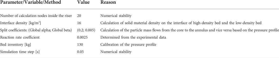
TABLE 5. Tuned parameter, variable, and method in the fluidized bed model.
4.3 Evaluation of tuned cases
To evaluate the tuning, the adjusted, steady-state cases of the simulation are compared with the corresponding experimental data at 60% and 80%. Both temperature and pressure profiles, as well as water, oxygen, and carbon dioxide content in the flue gas, are selected as points in comparison. The gas composition of the flue gas is evaluated before and after the cyclone separator. The data of the simulation in APROS can be read in the 20 calculation nodes. In each node, the material composition, temperature, and pressure in the corresponding area are given. In the experiment, pressure, and temperature sensors (see Table 6) are placed at different heights in the reactor.
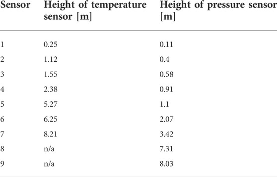
TABLE 6. Heights of the temperature and pressure sensors of the experiment (starting from the bottom of the reactor).
The first case considered is the second load case, which is one of the two set cases. Table 4 shows the input data of the simulation model for the simulated case. For validation, the pressure drops concerning the atmospheric pressure, the temperature profile, and the gas composition of the simulation are compared with the data of the experiment, and the deviations are evaluated. Figure 5 shows the pressure drop profiles of the second 60% and 100% load cases. The pressure of the simulation is shown as 1 bar since the respective pressure always applies to the entire height of the node. Here, the solid line performs the numerical results, while the red squares denote the experimental data. The simulated pressure profiles along the riser match the measurement after the mode tuning very well. In the heights between 2 and 4 m, the pressure drop in the simulation is slightly higher than the experimental values but is within a reasonable range. This indicates that the tuned model simulates the solid distribution in the bed very well for both load cases. The pressure profile in the 100% load case is about 7–12 mbar higher compared to the lower load case. It could be explained that the higher load case can increase the gases produced during combustion, resulting in higher pressure in the riser.
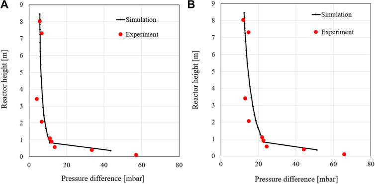
FIGURE 5. Pressure curves of the second load cases: 60% (A) and 100% (B).
The temperature profiles along the combustor at 60% and 100% load cases are shown in Figure 6. The simulated temperature profiles agree very well with the experimental. In the region of height between h = 0.25 and h = 2.5 m, the measured temperature is almost constant (about 780 °C) since a high number of solid particles and high content of oxygen concentrate at the bottom of the riser, resulting in a high mixing rate between solid fuels and oxygen. This suggests that more fuel is burned in the lower part of the riser. From the height of 2.74 m, the temperature in the riser starts decreasing, although the secondary air supplied (at heights of 2. m and 6 m) can promote the combustion of remaining char and volatile matter. It can be attributed to the non-preheated secondary air that could counteract the temperature increase from thermal heat released. Additionally, the reduction in temperature in the higher area is due to the cooling effect of the immersed water-cooled lances in the riser. Therefore, a slight decrease in temperature can be found in these regions.
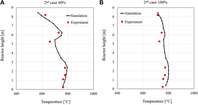
FIGURE 6. Temperature profiles of the second 60% (A) and 100% (B) load cases.
It should be noted that the model overestimates the measurement in most regions of the riser. It could be attributed to the assumptions of a good mixing rate between solid fuels and oxygen in the simulation, resulting in better and more complete combustion. Furthermore, the temperature profile of the 100% load case is higher than that of the 60% load case. This is due to the higher mass flow rate of solid fuels and air fed into the riser, which can promote the combustion process, resulting in higher thermal heat released in the riser.
The composition of the key flue gases (carbon dioxide, steam, and oxygen) at the outlet of the cyclone separator is illustrated in Figure 7. The simulation data is taken from the top node since this is the point closest to where the gas composition can be analysed. For the data of the experiment, the average value is taken over the load phase, while simulated values of the steady-state are used directly. The simulated contents agree very well with the measured data. It is noticeable that the oxygen content of the simulation is slightly higher than the oxygen content in the measurement for both load cases. However, the fraction of carbon dioxide in the experiment is higher than that in the simulation. The reason for this is probably that the experimental value is measured after leaving the reactor, while the simulation value describes the mean value at the top point of the riser. In the simulation, combustion still appears to be taking place at the point under consideration. However, the data agree well despite these deviations and the tuning can be assumed to be successful at this point.
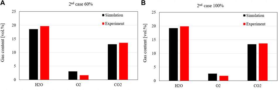
FIGURE 7. Gas composition of the second 60% (A) and 100% (B) load cases.
4.4 Steady-state model validation
To validate the steady-state load cases, this section compares the two unadjusted cases, the first 60% and first 100% load cases, with the corresponding experimental values. For further validation, the first and second 80% load cases are also compared with the corresponding experimental data.
4.4.1 Validation of first 60% load case
The first case considered for validating the system is the unadjusted 60% load case. Table 4 summarizes the input data of the simulation model for the first 60% load case. For validation, the pressure drop profile, the temperature profile and the flue gas composition obtained from the simulation are compared with the measured data, and then the deviations are evaluated.
As can be seen in Figure 8, the simulated pressure reproduces very well the measurement. A slight deviation can only be observed in the middle riser area, which is however still within a very good range. Furthermore, the figure compares the temperature profile of the simulation with that of the experiment in the first 60% load case. The simulated temperature is higher in the lower region of the riser than in the measurement, which indicates greater combustion in this area. In the upper region of the riser, a lower temperature is found in the simulation suggesting that most fuel has already been burned in the lower region of the riser. The explanation for this observation is the tuning of the mixing factors to the second load case to reduce carbon monoxide emission. A comparison of the boundary conditions of the two cases shows that the second 60% case has a higher coal mass flow rate than the first 60% case for the same air mass flow rate. This can be attributed to the fact that the mixing factors were increased for complete combustion of the fuel, but the combustion was promoted in the first case. However, the data are within acceptable limits and the experiment is well reproduced.
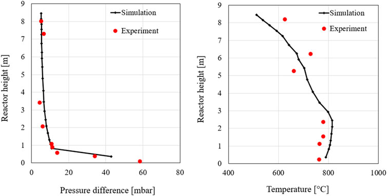
FIGURE 8. Pressure drop and temperature profiles along the riser at the first 60% load case.
The composition of the flue gas is also evaluated consistently with the previous section. Figure 9 illustrates the composition of the flue gas in the experiment at the outlet of the cyclone separator compared to the simulation data at the top calculation point. The proportions of steam and carbon dioxide in the experiment are higher than the simulated values. On the other hand, the oxygen concentration in the flue gas is slightly lower, which indicates that more fuel is burned. A possible explanation for this is that the numerical data do not indicate the values after the cyclone separator, but only represent the uppermost calculation range. Furthermore, it can be assumed that the fuel flow measurements used in the simulation may be subject to errors. However, the deviations are within a reasonable range and the simulation can be considered suitable for the simulation of this case.
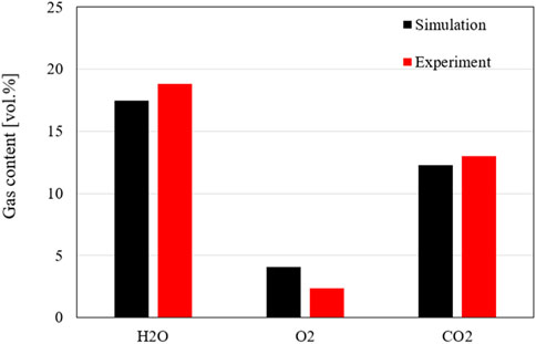
FIGURE 9. Gas composition of the first 60% load case.
4.4.2 Validation of first 100% load case
The second adapted case was simulated at 100% load. The corresponding boundary conditions are given in Table 4. The evaluation of the 100% load case is performed analogously to the previous sections.
The pressure and temperature curves are illustrated in Figure 10. As can be seen in these profiles, the measurement and simulation match each other very well. In the range of 2–4 m, slight deviations can again be observed in the pressure profile. However, these differences are within a very good range. This suggests a good simulation of the reactor mass distribution.
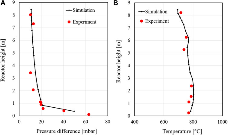
FIGURE 10. Pressure drop (A) and temperature (B) profiles at the first 100% load case.
The temperature curve of the first 100% load case shows that the simulation reproduces the experiment very well. The simulation data predict very well both, the temperatures in the lower reactor area as well as the temperature increase, due to the renewed combustion of volatile components and unconverted fuels, at the level of the secondary air. Therefore, the model performs a very good simulation of the combustion within the reactor for the first 100% load case. Thus, the simulation model can be considered validated at this point.
The gas composition of the first 100% load case shows a good agreement with the measured values, as shown in Figure 11. The deviations in the concentration of the flue gas species observed at the first 60% load case can also be found in this case. The explanation of these can still be used again at this point. However, the simulation data are generally close to the experimental data. The system can thus be considered validated for the first 100% load case.
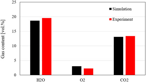
FIGURE 11. Gas composition of the first 100% load case.
4.4.3 Validation of 80% load cases
After the model tuning at 60% and 100% loads, to validate the steady-state load cases, the model was validated at 80% load against the corresponding measured data. It should be noted that because they are unadjusted and thus interpolated cases where the load is between the adjusted load cases. For this reason, these cases are useful for checking the methodology used to interpolate between the matched cases. Table 4 presents the boundary conditions of the first and second 80% load cases in the validation. The simulation results are evaluated through pressure profile, temperature profile, and flue gas composition at the cyclone.
Figure 12 illustrates the pressure drop profiles of the simulation and the measurement at the first and second 80% load cases, respectively. The model reproduces the experimental investigations very well with slight deviations which can be read in the middle range. Between h = 0 and 0.7 m, the pressure drop deviations are quite large, but the simulation results agree very well with the measurement at the height from h = 0.9 m. At the top of the riser, the simulation matches very well the measured value with about 5 mbar.
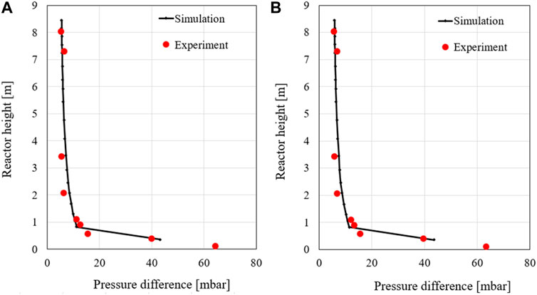
FIGURE 12. Pressure profiles at two 80% load cases: the first (A) and the second (B).
The temperature profiles along the combustor at two 80% load cases show good simulation results compared to the measured values (Figure 13). The model predicts the temperature accurately at the bottom and the top of the riser, while slight deviations can be observed in the middle part. It is noted that the model performs better in the second case. The reason for this temperature deviation in the simulation compared to the experimental data could be due to the location of the temperature sensor and the secondary air nozzles. In the test rig facility, temperature sensors are installed near the reactor walls. At the height of 6 m where the secondary air (2) is injected, the airflow at 25°C could cool down the temperature in the temperature sensors. Generally, the simulation temperatures are slightly higher than the measured value over most of the riser height. In the areas of the secondary air inflow, an increase in temperature can be seen due to higher oxygen content and the combustion of remaining char and volatile matter.
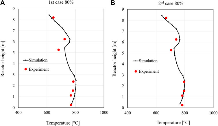
FIGURE 13. Temperature profiles along the riser at two 80% load cases: the first (A) and the second (B).
The flue gas fractions obtained from the simulation at the top of the riser match very well the measurement, shown in Figure 14. The model predicts the fraction of the gas species (CO2, O2, and H2O) with very high accuracy compared to the measured value in both cases. The measured gas fraction of carbon dioxide is about 12.8%, which is very close to the simulated value of 13%. Additionally, the model underestimates the steam fraction by about 0.6%, corresponding to a relative error of about 3%. However, there is a considerable deviation in the simulated oxygen concentration from the measurement with a relative error of about 33%, but the oxygen predicting error can be accepted since the oxygen concentration is still in the range of the minimum limit of the measurement.
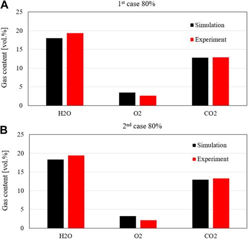
FIGURE 14. Flue gas concentrations at two 80% load cases: the first (A) and the second (B).
The simulated curves at the 80% load case are very similar and are close to the experimental values in different parameters, such as pressure, temperature, and flue gas composition. This shows that the model can be used well for predicting the temperature profile, even for non-adapted load cases in the stationary case.
Overall, the model performs very well in the steady-state simulation behaviour at various load cases. Temperature deviations are mostly within a range of 20°C and are within acceptable limits. The pressure profile is consistently well simulated, and only very few deviations are observed. The validation of the flue gas compositions found acceptable differences for oxygen, water, and carbon dioxide, which can be explained and are only within a small range. By tuning the second load cases for carbon monoxide reduction, the first cases have experienced a slight deterioration in the temperature curve. This is mostly due to higher mixing factors for the same total air mass flow rate and the lower fuel mass flow rate in the rear reactor.
4.5 Dynamic simulation validation
After the model was validated at various steady-state load cases, the dynamic simulation was carried out by changing the load as shown in Figure 15. The steady-state and transient behaviour of the simulated variables at different loads were validated against the measured data. It should be noted that the model is not tuned during load changes. The load change, shown in Figure 15, starts at the load of 60% remaining for about 125 min. Afterwards, the load increases to 80% and then to 100% within a few seconds, followed by steady-state phases for about 168 and 190 min, respectively. Finally, the load setpoint decreases from 100% to 80% and 60% before increasing to 100%.
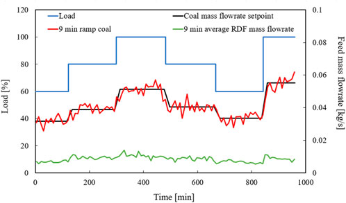
FIGURE 15. Dynamic curve of the fuel mass flow rate.
Figure 15 also illustrates the fuel mass flow curve corresponding to the dynamic simulation load curve. Here, the coal mass flow is shown as the setpoint and 9-min average of the values measured in the experiment, both of which are used in the dynamic history simulation. The RDF mass flow is also given as the 9-min average of the values measured in the experiment. The 9-min average of the coal mass flow rate follows the setpoint well. However, it is noticeable that the transient steps between the load setpoint specification in the area around the load jumps have a slope instead of a jump, which can be attributed to the interpolation between the average values of the individual load steps. Following the 9-min average despite the interpolation between load steps, indicates poor calculation of the coal mass flow. Nevertheless, the values are acceptable and will continue to be used for dynamic simulation. The RDF curve does not clearly show any transient step, but the following of the load curve can still be seen.
To validate the dynamic simulation, the temperature profile of the riser at two different heights is first compared with the measured values (see Figure 16). As heights, a point at the height of 2.38 m, which represents the lower part of the riser (bed zone) with high particle density, and a point at the height of 8.21 m were chosen. The second point is particularly meaningful because it is located at the highest calculation point of the simulation and thus indicates the temperature of the flue gas leaving the cyclone separator into the heat exchangers. Thus, it is a good comparison value, since it plays a decisive role in the design of a power plant.
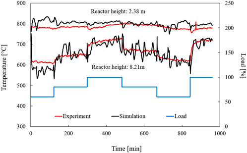
FIGURE 16. Temperature profiles of the dynamic simulation at different heights in the riser.
As can be seen from the measured temperature at the height of 2.38 m, it is noted that no clear delimitations of the load cases can be observed. However, a slope around the 100% load case can be found. The simulated temperatures at the corresponding height are mostly higher than the experimental values. This is especially true for the first case, which agrees with the assumption that the combustion in the bed zone of the riser increases in the first case. The reason for this is the increase in the mixing factors due to the CO tuning. However, the temperature differences are in a very small range concerning the absolute temperature. At the height of 8.21 m, the load changes can be seen well in the change in temperature curve. It should be noted that the temperature profile of the simulation at the corresponding height follows the jumps well. However, larger fluctuations of the simulated temperature can also be seen, which can be attributed to different reasons.
One possible explanation is that the calculation of the fuel mass flow rate has its challenges due to the intermittent input of the fuel in the experiment. One effect of an incorrectly calculated fuel mass flow can be an overestimation of the peaks of the mass flow. Another reason for the fluctuations could be too fast combustion of the fuel in the simulation, while in the experiment the addition of carbon, due to a slow conversion may be slower. Another reason could be that in the simulation, due to the influence of the deviations between the actual value of the carbon stream and the target value of the carbon stream, the mixing factors increase too fast, resulting in a significant increase in the combustion. Despite the fluctuations, the simulated profile matches the measurement very well at this level. It can be concluded that the temperature in the reactor can also be reproduced well in dynamic simulations.
To investigate the fluctuations of the temperature at the top calculation point of the simulation, the temperature curve of simulation and measurement are compared with the mass flow of coal from the 500th minute to the 700th minute. This time range was chosen because particularly strong fluctuations were found there. Figure 17 shows that there is no direct influence of the coal mass flow fluctuations on the temperature and therefore no direct correlation between the two parameters. Therefore, it must be assumed that other influences are causing the temperature fluctuations. Further investigations are therefore necessary to determine the exact cause of the fluctuations. However, it cannot be excluded that an improvement of the coal mass flow, through more accurate measurements, also results in a better temperature curve. Despite the fluctuations, the model performs very good simulation properties for the temperature of the dynamic simulation of a co-combustion of coal and RDF.
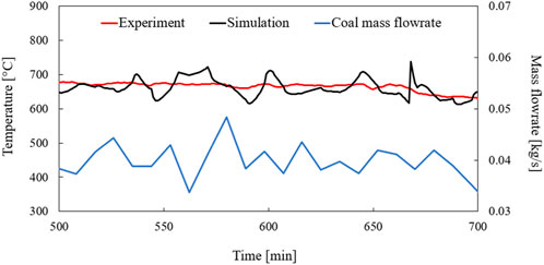
FIGURE 17. Comparison of the temperature fluctuations with the coal stream.
The last point considered in this section is the heat transfer between the reactor and the cooling lances. This is represented by the temperature increase of the cooling water flowing through the cooling lances. Figure 18 shows the temperature difference between simulation and experiment in comparison to the load course of the dynamic simulation. As can be seen, the simulated profile matches that of the experiment very well. However, the numerical temperature is always higher than that of the experiment. This temperature difference can be explained by the fact that the cooling water in the experiment flows through an uncooled pipe system before measuring temperature. Since the temperature loss cannot be measured at this point, it results that the calculated temperatures must be higher than the measured values. However, the fact that the curves are similar and follow the load suggests that the simulation can also reproduce the heat transfer to the cooling lances well.
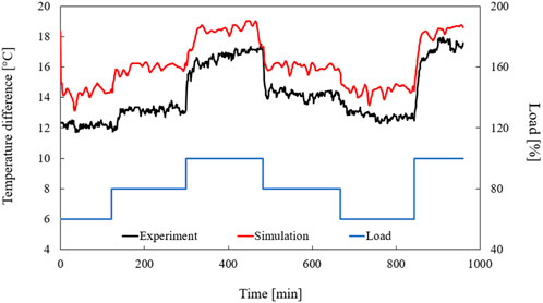
FIGURE 18. Comparison of the temperature difference of the cooling water of the cooling lances.
Overall, the simulation shows good behaviour in the dynamic simulation of the co-combustion of coal and RDF. There are no significant deviations observed. Therefore, the simulation model, for the co-combustion of coal and RDF, is sufficiently validated. In the further course of this elaboration, the simulation model has therefore considered a good approximation to the real reactor.
4.6 Increase of RDF share
After validating, the simulation model is used to investigate the increase of RDF fuel mass fraction and the increase of RDF load fraction in a CFB reactor. Individual cases with different RDF fractions are simulated in steady-state conditions and compared with each other.
4.6.1 Boundary conditions at various RDF mass fractions
In the same experiment series in which the dynamic test of co-combustion of coal and RDF has been performed, two steady-state measurements of different RDF fuel fractions have also been carried out. The numerical results of these cases are considered in this section and compared with the experimental data. Table 7 presents the boundary conditions used for the steady-state cases of the measurement. In each case, the values are the calculated mean values of the steady-state operation in the experimental investigation.
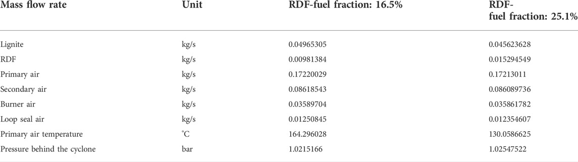
TABLE 7. Boundary conditions of the steady-state simulation with 16.5% and 25.1% RDF.
The fraction of RDF is given corresponding to the total fuel mass flow, i.e., the sum of RDF and coal mass flow. Table 7 shows that the airflow rates of the two cases are almost identical. Therefore, for the other steady-state cases selected, the boundary conditions of the 25.1% RDF fraction case were retained and only the RDF and coal fuel mass flows were changed. As a rough estimate, the total fuel mass flow was also kept constant while the RDF fraction varied. This approach is only a rough estimate because the fuels may require different amounts of air for complete combustion and therefore this approach may result in incomplete combustion within the riser. This estimation was made both due to time constraints as per the agreement and for simple estimation of the behaviour of the simulation model when fuel ratios change. Proportions of 30%, 50%, 80%, and 99% were chosen for the RDF fuel mass fractions for further investigation.
Table 8 shows the individual RDF proportions selected in the simulation and the associated fuel mass flows. The mass flows are calculated as a fraction of the total mass flow of the 25.1% RDF fraction case.
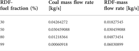
TABLE 8. Fuel mass flows as a function of the RDF fuel.
4.6.2 Evaluation for higher RDF mass fractions
To evaluate the simulation results, the temperature and pressure profiles of the simulated steady-state cases are compared with the measured data. Figure 19 shows the temperature and pressure profiles of the simulation at an RDF fuel mass fraction of 16.5% and 25.1%, respectively, which are compared to the measured values in the experimental series. The pressure profiles of the simulation show a good agreement with the experimental data. Thus, the mass distribution is well reproduced even with the variations of the RDF fraction. Furthermore, the temperature profiles of the two cases, also match the experimental data well. However, slight temperature deviations can be observed here, but they are within reasonable limits. The pressure increases at an RDF fuel mass fraction of 25.1% in the upper region compared to the 16.5% case. Additionally, an increased temperature is found in the top region of the riser at a higher RDF fraction. This observation is consistent with the pressure profile data.
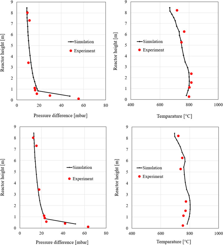
FIGURE 19. Pressure and temperature profiles at 16.5% and 25.1% RDF fuel mass fraction.
Two approaches can be considered to explain this behaviour. First, the RDF fuel consists of easily fluidizable solid particles (paper, foil, etc.), which can be discharged more easily from the bed in the riser and can thus cause a larger mass fraction in the upper reactor section. With this explanation, it is questionable whether the simulation model can simulate this easier discharge since the shape of the particles cannot be precisely defined and only the density of the particles and their size are adjusted. The second approach considers the difference in the proportions of volatiles in coal and RDF. RDF has a larger proportion of volatile matters, which also rise in the combustion chamber where they are burned in the upper region. This behaviour can lead to both a higher temperature and a slightly higher pressure inside the riser.
To further verify the increase in RDF fuel mass fraction, the temperature and pressure curves of steady-state simulations at 30%, 50%, 80%, and 99% RDF fuel mass fraction (see Table 8) are compared as shown Figure 20. The temperature in the upper region of the combustion chamber continues to increase up to approximately a value of 50% RDF. The pressure in the upper area also increases with increasing RDF fuel fraction. However, a further increase in the RDF fraction does not lead to any further temperature increases in the simulation. A precise evaluation of the differences in temperature and pressure between the individual cases based on the curves plotted against the reactor height is difficult.
FIGURE 20. Pressure and temperature profiles at 30%, 50%, 80% and 99% RDF fuel.
For a better assessment of the pressure at different RDF fuel mass fractions, Figure 21 shows the pressure differences to ambient pressure at a height of 2.455 m concerning the RDF fraction in the fuel mass. The height was selected since the particles have already been carried out of the solid bed at this point. However, there is still a high particle density at this point, so the course of the pressure differences is visible. A significant increase in pressure can be observed between the 16.5% and 25.1% RDF fuel mass fraction. This can be explained by deviating boundary conditions as shown in Table 7. The other data show a clear increasing trend, indicating that a larger number of particles are discharged from the reactor bed. However, whether these consist of RDF particles or volatiles cannot be determined from the model.
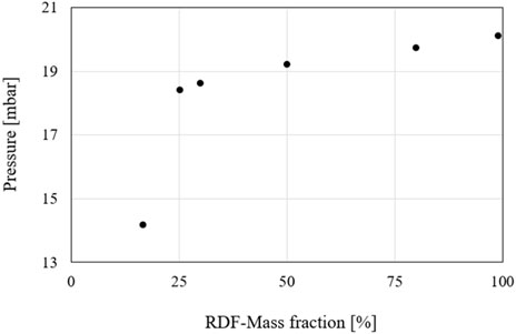
FIGURE 21. Comparison of pressures at 2.455 m concerning RDF fuel mass fraction.
As a further consideration, Figure 22 plots the temperatures of the upper calculation point concerning the RDF fuel fraction. This point is selected since it can be used as a good approximation of the temperature at the outlet of the cyclone separator. There is a considerable increase in temperature between the 16.5% and 50% RDF fuel mass fraction. These values support the proposition that the RDF has a greater proportion of combustible volatiles that are burned at the top of the riser. However, as the RDF fraction increases further above 50%, the temperature is mostly unchanged. One explanation of this behaviour is the mismatched air mass flow of the simulation. In this case, the temperature does not increase further because fuel is still present, but no oxygen is available for complete combustion.
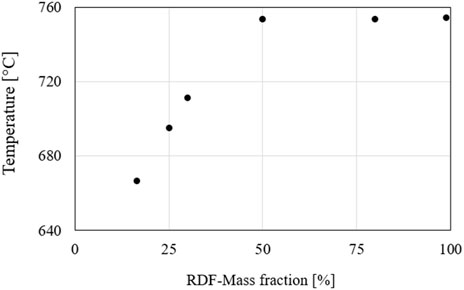
FIGURE 22. Comparison of temperatures at 8.45 m concerning RDF fuel mass fraction.
To investigate the absence of a further increase in temperature, the flue gas is evaluated for unburned fuels. Table 9 gives the mole fractions of methane and carbon monoxide at the top calculation point of the riser. The fraction of volatiles unburned increases from an RDF fuel fraction of 50%. This indicates that the combustion, at the time of the exit of the flue gas from the cyclone separator, is not yet finished. Therefore, the temperature and pressure values of the simulation do not correspond to the values when the fuel is completely burned (an adjustment of the air flows is necessary to obtain correct values).
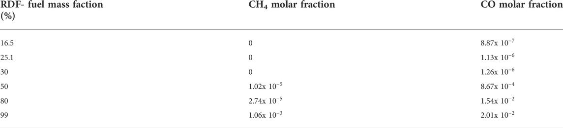
TABLE 9. Molar fractions of methane and carbon monoxide in the flue gas.
An evaluation of the cases without experimental data shows that increasing the RDF fuel mass fraction also increases the total reactor load. Figure 23 shows the total load of the fuel mass flows for the respective cases of RDF fuel mass fraction. The load, with the total mass fuel flow remaining constant and the RDF fuel mass fraction increasing, is steadily increasing. The reason for this is the higher lower heating value of RDF compared to coal. It cannot be ruled out that this increase in total load leads to the observed incomplete combustion.
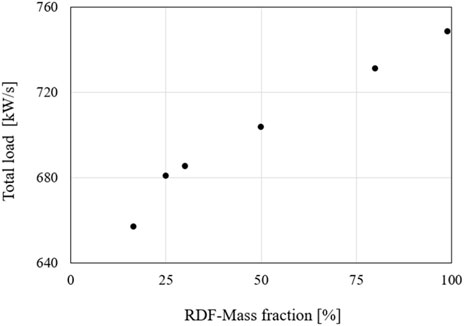
FIGURE 23. Comparison of the total load concerning the RDF fuel mass fraction.
4.6.3 Investigation of increase of the RDF load share
The RDF load fraction is defined as the share of the calorific value of RDF in the total calorific value of the fuels. For the investigation of the increase of the RDF load fraction, the same steady-state load cases are used as a basis as in the previous section. The evaluation presented there still holds since the simulation of the two cases uses the boundary conditions of the measurements in the experiment. However, it should be noted that the 16.5% RDF fuel mass fraction corresponds to an RDF load fraction of 18.4%, while the 25.1% RDF fuel mass fraction corresponds to an RDF load fraction of 27.6%. Furthermore, the boundary conditions of the 27.6% RDF load fraction case were again used for the estimation. A 40%, a 60%, 80%, and a 100% RDF load share case are selected for the study. Table 10 shows the simulation values used for the fuel flow. The other boundary conditions are given in Table 7 under 25.1% RDF fuel mass fraction (corresponding to an RDF load fraction of 27.6%).

TABLE 10. Fuel mass flows of the increase in RDF load share.
Figure 24 shows the pressure and temperature profiles of the simulated steady-state cases at various RDF load fractions. In the comparison, significant differences in the curves can be observed.
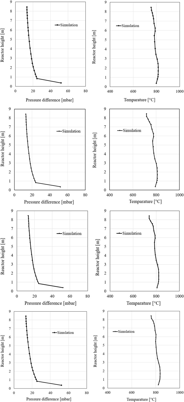
FIGURE 24. Pressure and temperature profile at 40%, 60%, 80% and 100% RDF load share.
To further investigate the differences between the respective simulations, the temperatures at the uppermost calculation point at 8.45 m and the pressures of the calculation point at a height of 2.455 m are compared. Figure 25 shows the comparison of the pressures and the comparison of temperatures at the highest calculation point of the simulation model for varying the RDF load fraction. The pressures continue to show a steady increase and are very similar to the pressures of varying the RDF fuel fraction illustrated in Figure 21. This observation leads to the conclusion that the increase in pressure is mainly generated by the larger volatile content in the RDF or the lighter particles and occurs independently of the increase in total load. Unlike the values observed in Figure 22, the temperature increases as the RDF load fraction increases, but does not stagnate. A comparison of the final values of both figures shows that the final temperature value of the RDF load fraction increase approximates the temperature of stagnation in Figure 22. While the stagnation in the original case can be attributed to the increase in load and the accompanying sub-stoichiometric combustion, incomplete combustion does not occur at any point in the case of the simulation of the increased RDF load fraction. The temperature increase in the upper part of the reactor can be attributed to the higher volatile fuel fraction and the easier discharge of RDF particles.
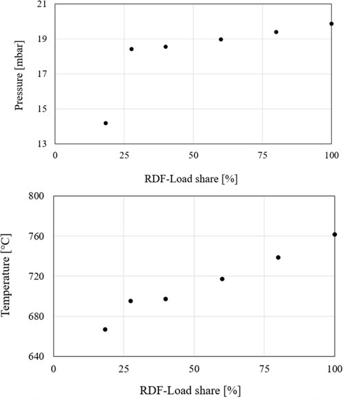
FIGURE 25. Pressure (at 2.455 m) and temperature (at 8.45 m) by variation of the RDF load fraction.
The studies on the increases in RDF fuel mass fraction and RDF load fraction show that the simulation model produces plausible data even for unadjusted changes in fuel composition. Despite the erroneous design of the boundary conditions, the results are meaningful. A positive aspect is the recognizability of the different behaviour of different fuels. Both pressure and temperature also vary when the fuel composition is changed.
Overall, it can be seen in this case that the temperature profile is well reproduced. This indicates that small adjustments to the system will allow further improved simulation of real conditions. However, due to time constraints, this was not considered further in this work after consultation.
Furthermore, it can be observed that the mass distribution and thus also combustion shifts slightly to the upper region of the riser due to a higher RDF fraction. This observation supports the assumption that the RDF fuel contains more volatile fractions than coal. These rise faster in the reactor and are combusted in the upper region, providing a higher temperature and pressure. It should be noted that the boundary conditions of the simulation for an RDF share above 25.1% were only estimated and further tests on the real reactor are necessary to validate the simulation model.
5 Conclusion
A dynamic process simulation of an existing 1 MWth CFB plant was developed in APROS software to investigate the operational flexibility of lignite and refuse-derived fuel (RDF) co-combustion at various partial loads. The modelling procedure includes tuning, validation, and applications under steady-state and transient conditions. The following conclusions can be obtained:
1. The model reproduces accurately the most important parameters during the long-term test campaign for the dynamic simulation and provides reliable results. There are some slight deviations, but they are within acceptable limits.
2. The developed model shows very good behaviour for the steady-state cases. Temperature deviations are mostly within a range of 20 °C and are within acceptable limits. The pressure profile is consistently well simulated and shows only minor deviations. The comparison of the gas compositions shows equal differences for oxygen, water, and carbon dioxide, which can be explained well and are only within a small range.
3. The developed model performs good behaviour in the dynamic simulation of the co-combustion of lignite and RDF. There are no deviations that cannot be explained. Therefore, the simulation model, for the co-combustion of coal and RDF, is sufficiently validated.
4. In the investigation of the increasing share of RDF, the mass distribution and the combustion shift slightly to the upper region of the combustion chamber due to a higher RDF fraction. This observation supports the assumption that the RDF fuel contains more volatile fractions than coal. These rise faster in the reactor and are burned in the upper region, providing a higher temperature and pressure.
The simulation model can be used to predict the behaviour of a CFB reactor for simulating the co-combustion of lignite and RDF. The model promises to be a good alternative in the future for estimating the behaviour of the reactor at boundary conditions not previously studied experimentally. The rapid and cost-effective investigation of many, different operating cases of the CFB reactor can thus provide important insights into how circulating fluidized bed combustion can be operated in the most environmentally friendly and flexible way. They thus make a decisive contribution to the integration of renewable power generators while guaranteeing the security of supply.
Data availability statement
The datasets generated for this study are available on request to the corresponding author.
Author contributions
FA and NN are responsible for administration, conceptualization, the original draft, and the applied methodology. BJ developed and validated the model. The experimental investigations were managed and conducted by JP. FA, and AK supported the writing process with their reviews and edits. BE supervised the research progress and the presented work. All authors have read and agreed to the published version of the manuscript.
Funding
Financial support is acknowledged from the Research Fund for Coal and Steel (RFCS) project of the European Commission under grant agreement n. 101034024 (Retrofitting Fluidized Bed Power Plants for Waste-Derived Fuels and CO2 Capture).
Acknowledgments
We acknowledge support from the Deutsche Forschungsgemeinschaft (DFG) German Research Foundation and the Open Access Publishing Fund of the Technical University of Darmstadt.
Conflict of interest
The authors declare that the research was conducted in the absence of any commercial or financial relationships that could be construed as a potential conflict of interest.
Publisher’s note
All claims expressed in this article are solely those of the authors and do not necessarily represent those of their affiliated organizations, or those of the publisher, the editors and the reviewers. Any product that may be evaluated in this article, or claim that may be made by its manufacturer, is not guaranteed or endorsed by the publisher.
Abbreviations
AEA, Atomic Energy Agency; BFB, Bubbling fluidized bed; CCE, Carbon conversion efficiency; CGE, Cold gas efficiency; DIN, Deutschen Instituts für Normung; ER, Equivalence ratio; H/C, Hydrogen-to-carbon ratio; LHV, Lower heating value; O/C, Oxygen-to-carbon ratio; PI, Pressure indicator; Syngas, Synthesis gas; SBR, Steam-to-biomass ratio; TI, Temperature indicator.
References
Al-Maliki, W. A. K., Alobaid, F., Kez, V., and Epple, B. (2016). Modelling and dynamic simulation of a parabolic trough power plant. J. Process Control 39, 123–138. doi:10.1016/j.jprocont.2016.01.002
Al-Maliki, W. A. K., Alobaid, F., Starkloff, R., Kez, V., and Epple, B. (2016). Investigation on the dynamic behaviour of a parabolic trough power plant during strongly cloudy days. Appl. Therm. Eng. 99, 114–132. doi:10.1016/j.applthermaleng.2015.11.104
Alobaid, F., Al-Maliki, W. A. K., Lanz, T., Haaf, M., Brachthäuser, A., Epple, B., et al. (2018). Dynamic simulation of a municipal solid waste incinerator. Energy 149, 230–249. doi:10.1016/j.energy.2018.01.170
Alobaid, F., Almohammed, N., Farid, M. M., May, J., Rößger, P., Richter, A., et al. (2021). Progress in CFD simulations of fluidized beds for chemical and energy process engineering. Prog. Energy Combust. Sci. 91, 100930. doi:10.1016/j.pecs.2021.100930
Alobaid, F., Mertens, N., Starkloff, R., Lanz, T., Heinze, C., and Epple, B. (2017). Progress in dynamic simulation of thermal power plants. Prog. Energy Combust. Sci. 59, 79–162. doi:10.1016/j.pecs.2016.11.001
Alobaid, F., Peters, J., Amro, R., and Epple, B. (2020). Dynamic process simulation for Polish lignite combustion in a 1MWth circulating fluidized bed during load changes. Appl. Energy 278, 115662. doi:10.1016/j.apenergy.2020.115662
Alobaid, F., Postler, R., Ströhle, J., Epple, B., and Kim, H-G. (2008). Modeling and investigation start-up procedures of a combined cycle power plant. Appl. Energy 85, 1173–1189. doi:10.1016/j.apenergy.2008.03.003
Angerer, M., Kahlert, S., and Spliethoff, H. (2017). Transient simulation and fatigue evaluation of fast gas turbine startups and shutdowns in a combined cycle plant with an innovative thermal buffer storage. Energy 130, 246–257. doi:10.1016/j.energy.2017.04.104
Arkoma, A., Hänninen, M., Rantamäki, K., Kurki, J., and Hämäläinen, A. (2015). Statistical analysis of fuel failures in large break loss-of-coolant accident (LBLOCA) in EPR type nuclear power plant. Nucl. Eng. Des. 285, 1–14. doi:10.1016/j.nucengdes.2014.12.023
Bany Ata, A., Alobaid, F., Heinze, C., Almoslh, A., Sanfeliu, A., and Epple, B. (2020). Comparison and validation of three process simulation programs during warm start-up procedure of a combined cycle power plant. Energy Convers. Manag. 207, 112547. doi:10.1016/j.enconman.2020.112547
Castilla, G. M., Montañés, R. M., Pallarès, D., and Johnsson, F. (2021). Dynamic modeling of the reactive side in large-scale fluidized bed boilers. Ind. Eng. Chem. Res. 60, 3936–3956. doi:10.1021/acs.iecr.0c06278
Chen, Y., and Xiaolong, G. (2006). Dynamic modeling and simulation of a 410t/h Pyroflow CFB boiler. Comput. Chem. Eng. 31, 21–31. doi:10.1016/j.compchemeng.2006.04.006
Daikeler, A. (2019). Experimentelle Untersuchung der Partikelströmung in zirkulierenden Wirbelschichten mittels eines kapazitiven Messsystems [Ph.D.]. Munich, Germany: German National Library of Science and Technology: Technische Universität Darmstadt.
Gungor, A., and Eskin, N. (2007). Analysis of environmental benefits of CFB combustors via one-dimensional model. Chem. Eng. J. 131, 301–317. doi:10.1016/j.cej.2006.12.012
Gungor, A. (2009). One dimensional numerical simulation of small scale CFB combustors. Energy Convers. Manag. 50, 711–722. doi:10.1016/j.enconman.2008.10.003
Haenninen, M. Phenomenological extensions to APROS six-equation model Non-condensable gas, supercritical pressure, improved CCFL and reduced numerical diffusion for scalar transport calculation. Finland2009, 60.
Henrion, T., Ponweiser, K., Band, D., and Telgen, T. (2013). Dynamic simulation of a solar power plant steam generation system. Simul. Model. Pract. Theory 33, 2–17. doi:10.1016/j.simpat.2011.12.009
Hentschel, J., Zindler, H., and Spliethoff, H. (2017). Modelling and transient simulation of a supercritical coal-fired power plant: Dynamic response to extended secondary control power output. Energy 137, 927–940. doi:10.1016/j.energy.2017.02.165
Hiidenkari, H., Tuuri, S., Lappalainen, J., and Ritvanen, J. (2019). Dynamic core-annulus model for circulating fluidized bed boilers.
Hotta, A. (2010). “Foster wheeler’s solutions for large scale CFB boiler technology: Features and operational performance of lagisza 460 MWe CFB boiler,” in Proceedings of the 20th international conference on fluidized bed combustion. Editors G. Yue, H. Zhang, C. Zhao, and Z. Luo (Berlin, Heidelberg: Springer Berlin Heidelberg), 59–70.
Kumar, H., Mohapatra, S. K., and Singh, R. I. (2018). Review on CFD modelling of fluidized bed combustion systems based on biomass and co-firing. J. Inst. Eng. India. Ser. C 99, 449–474. doi:10.1007/s40032-017-0361-2
Kunii, D., and Levenspiel, O. (1991). “Fluidization engineering,” in Fluidization engineering. Editors D. Kunii, and O. Levenspiel. Second Edition (Boston: Butterworth-Heinemann), 491.
Lappalainen, J., Lalam, V., Charreire, R., and Ylijoki, J. (2017). Dynamic modelling of a CFB boiler including the solids, gas and water-steam system.
Lappalainen, J., Tourunen, A., Mikkonen, H., Hänninen, M., and Kovács, J. (2014). Modelling and dynamic simulation of a supercritical, oxy combustion circulating fluidized bed power plant concept—firing mode switching case. Int. J. Greenh. Gas Control 28, 11–24. doi:10.1016/j.ijggc.2014.06.015
Luo, W., Wang, Q., Huang, X., Liu, Z., and Zheng, C. (2015). Dynamic simulation and transient analysis of a 3MWth oxy-fuel combustion system. Int. J. Greenh. Gas Control 35, 138–149. doi:10.1016/j.ijggc.2015.02.003
Magnussen, B. F., and Hjertager, B. H. (1977). On mathematical modeling of turbulent combustion with special emphasis on soot formation and combustion. Symposium Int. Combust. 16, 719–729. doi:10.1016/s0082-0784(77)80366-4
Mertens, N., Alobaid, F., Lanz, T., Epple, B., and Kim, H-G. (2016). Dynamic simulation of a triple-pressure combined-cycle plant: Hot start-up and shutdown. Fuel 167, 135–148. doi:10.1016/j.fuel.2015.11.055
Mertens, N. J., Alobaid, F., Epple, B., and Kim, H-G. (2016). “Combined-cycle start-up procedures: Dynamic simulation and measurement,” in ASME 2016 power conference collocated with the ASME 2016 10th international conference on energy sustainability and the ASME 2016 14th international conference on fuel cell science (Charlotte: Engineering and Technology).
Mikkonen, H., Lappalainen, J., and Kuivalainen, R. (2015). Modelling and dynamic studies of the second generation oxy-fired CFB boiler.
Pan, J., Yang, D., Chen, G., Zhou, X., and Bi, Q. (2012). Thermal-hydraulic analysis of a 600 MW supercritical CFB boiler with low mass flux. Appl. Therm. Eng. 32, 41–48. doi:10.1016/j.applthermaleng.2011.08.009
Peters, J., Alobaid, F., and Epple, B. (2020). Operational flexibility of a CFB furnace during fast load change—experimental measurements and dynamic model. Appl. Sci. 10, 5972. doi:10.3390/app10175972
Schuhbauer, C., Angerer, M., Spliethoff, H., Kluger, F., and Tschaffon, H. (2014). Coupled simulation of a tangentially hard coal fired 700°C boiler. Fuel 122, 149–163. doi:10.1016/j.fuel.2014.01.032
Starkloff, R., Alobaid, F., Karner, K., Epple, B., Schmitz, M., and Boehm, F. (2015). Development and validation of a dynamic simulation model for a large coal-fired power plant. Appl. Therm. Eng. 91, 496–506. doi:10.1016/j.applthermaleng.2015.08.015
Starkloff, R., Postler, R., Al-Maliki, W. A. K., Alobaid, F., and Epple, B. (2016). Investigation into gas dynamics in an oxyfuel coal fired boiler during master fuel trip and blackout. J. Process Control 41, 67–75. doi:10.1016/j.jprocont.2016.03.003
Tang, G., Zhang, M., Gu, J., Wu, Y., Yang, H., Zhang, Y., et al. (2019). Thermal-hydraulic calculation and analysis on evaporator system of a 660 MWe ultra-supercritical CFB boiler. Appl. Therm. Eng. 151, 385–393. doi:10.1016/j.applthermaleng.2019.01.060
Wang, L., Yang, D., Shen, Z., Mao, K., and Long, J. (2016). Thermal–hydraulic calculation and analysis of a 600 MW supercritical circulating fluidized bed boiler with annular furnace. Appl. Therm. Eng. 95, 42–52. doi:10.1016/j.applthermaleng.2015.11.014
Wang, Q., Luo, Z., Li, X., Fang, M., Ni, M., and Cen, K. (1999). A mathematical model for a circulating fluidized bed (CFB) boiler. Energy 24, 633–653. doi:10.1016/s0360-5442(99)00008-0
Wu, H., Yang, C., He, H., Huang, S., and Chen, H. (2018). A hybrid simulation of a 600 MW supercritical circulating fluidized bed boiler system. Appl. Therm. Eng. 143, 977–987. doi:10.1016/j.applthermaleng.2018.07.102
Yang, H., Yue, G., Xiao, X., Lu, J., and Liu, Q. (2005). 1D modeling on the material balance in CFB boiler. Chem. Eng. Sci. 60, 5603–5611. doi:10.1016/j.ces.2005.04.081
Keywords: 1 MWth circulating fluidized bed test facility, dynamic simulation, co-combustion, load change, validation study
Citation: Alobaid F, Kuhn A, Nguyen NM, Johnen B, Peters J and Epple B (2022) Numerical and experimental study of co-combustion of refuse-derived fuels in a circulating fluidized bed during load change. Front. Energy Res. 10:969780. doi: 10.3389/fenrg.2022.969780
Received: 15 June 2022; Accepted: 11 July 2022;
Published: 04 October 2022.
Edited by:
Piero Salatino, University of Naples Federico II, ItalyReviewed by:
A. Dhaundiyal, Hungarian Academy of Sciences (MTA), HungaryJiaying Pan, Tianjin University, China
Copyright © 2022 Alobaid, Kuhn, Nguyen, Johnen, Peters and Epple. This is an open-access article distributed under the terms of the Creative Commons Attribution License (CC BY). The use, distribution or reproduction in other forums is permitted, provided the original author(s) and the copyright owner(s) are credited and that the original publication in this journal is cited, in accordance with accepted academic practice. No use, distribution or reproduction is permitted which does not comply with these terms.
*Correspondence: Falah Alobaid, RmFsYWguQWxvYmFpZEBlc3QudHUtZGFybXN0YWR0LmRl