Anomaly electricity detection method based on entropy weight method and isolated forest algorithm

1 Introduction

With the rapid development of smart grid technology, the electricity consumption information collection system and distribution automation system have been improved, smart meters are popular, where the data center has also been gradually established and improved, and the collected power consumption data of the user end shows the characteristics of large scale, various types, and fast growth rate (Song et al., 2016). At the same time, some users steal electricity which causes huge income loss in the power company. Common ways of stealing electricity include: stealing electricity by changing the current, stealing electricity by changing the voltage, stealing electricity by changing the structure and wiring method of the meter, and stealing electricity by strong AC magnetic fields. Their common feature is to change the real value of electricity consumption to achieve the purpose of less metering or no metering. Therefore, the behavior of stealing electricity will lead to an error between the meter measurement of the station and the total meter measurement. With the development of deep learning technology and intelligent algorithms, it is possible to analyze user behavior, mine data hidden features and electricity consumption trends (Zhang et al., 2021). Therefore, it is of great significance to ensure the normal operation of the power system to make full use of the massive user power consumption data, mine and analyze the intrinsic value of the data through intelligent algorithms, and to improve the detection efficiency and accuracy of electricity theft (Liu et al., 2020).

Reference (Monedero et al., 2012) uses the Pearson correlation coefficient to detect typical NTL characterized by a sudden load drop, and for other types of NTL, it is detected by Bayesian network and decision tree. Reference (Nizar et al., 2008) first obtained the characteristic curve of each type of user by clustering the user load curve, and then divided the users into two categories: normal and abnormal according to the degree of deviation between the load curve and the characteristic curve, and finally predicted new users with extreme learning machine. type. Reference (Angelos et al., 2011) proposed an NTL detection method based on fuzzy C-means clustering. Reference (Zheng et al., 2019) combines the correlation analysis of line loss and the rapid clustering of density peaks for daily load curves to detect electricity theft by users. Reference (Zheng et al., 2018) and Reference (Hu et al., 2019) use a deep convolutional neural network (CNN) and a support vector machine based on stacked decorrelation autoencoders, respectively, to identify electricity stealing users based on load time series data. Reference (Zhang, 2014) uses the kernel function to map the dataset to the feature space, and calculates the outlier factor in the feature space, which is applicable to a wider range of datasets. Reference (Zhuang et al., 2016) proposes an anomaly detection method based on unsupervised learning, and uses grid processing technology to improve the LOF algorithm, which improves the efficiency of the algorithm.

The above work provides a strong theoretical basis for the detection of electricity stealing behavior, but the research on abnormal electricity consumption detection at home and abroad still needs to be in-depth. Abnormal power consumption detection is reflected in the current research mainly using an optimized recognition model driven by accuracy. Abnormal samples with low weights are easily ignored, resulting in a low recall rate, and the effect of effectively detecting abnormal samples cannot be achieved.

The conventional anomaly detection problem is a typical binary classification problem. Usually, the number of abnormal data samples is much smaller than the number of normal samples. Therefore, the model is also required to have high adaptability to imbalanced data sets (Mortaz, 2020). The detection of abnormal power consumption behavior can also be classified as a two-category problem, that is, only judging whether the user uses abnormal power consumption, and conducting in-depth classification research on the categories of abnormal user data. For the abnormal detection problem scenario, abnormal electricity users only account for a small part, so it is the imbalance learning problem. For the imbalance problem, we should not only use the accuracy rate as the model evaluation index, but also pay more attention to the recall rate and other indicators to measure the effect of abnormal sample detection. Commonly used evaluation metrics include precision, recall, confusion matrix, receiver operating characteristic curve (ROC), and F1-Score (Kim et al., 2007).

The power load anomaly detection model usually includes two modules: feature construction and anomaly detection (Rajendran et al., 2019; Zhang et al., 2020). The process of power load anomaly detection model in this paper is: feature construction-dimension reduction-clustering-anomaly detection. Since different types of electricity users (such as urban resident users, rural resident users, industrial and commercial users, etc.) often have different types of electricity consumption patterns, the k-means clustering algorithm (Xu et al., 2015) is firstly used as the classification model to complete the rough classification of users; then the entropy weight Method (Song et al., 2019) is introduced. The weight value of the whole abnormal score determined by different features is evaluated by the method; finally, the feature-weighted isolated forest algorithm is used to obtain the abnormal users of electricity consumption.

2 Anomaly detection model

2.1 K-means algorithm

The abnormal power consumption detection method adopts the power consumption data of all power users to detect ill behaviors. On the one hand, since different types of users have different power consumption behaviors, an abnormal user may be distributed in the cluster of another type of normal users. There is little difference in the electricity consumption behavior of Class B users. Since the electricity consumption habits of different users may change, a normal user of Class A may have similar electricity consumption behavior to that of Class B users in a certain period of time, so it is classified into Class B in the user’s cluster. On the other hand, the electricity consumption behavior of Class A users is quite different from that of Class B users. However, due to the abnormal electricity consumption behavior of some abnormal users of Class A, their electricity consumption behavior changes, which may be similar to those of Class B users, so they are classified into in a cluster of class B users. Therefore, after the dimensionality reduction by principal component analysis, the abnormal user may be distributed in another type of normal user cluster, and thus be misjudged as a normal user. After the users are classified, since the electricity consumption behaviors of similar users are similar, the above-mentioned problems do not exist in abnormal detection of each type of users, and the detection accuracy can be improved.

The k-means algorithm is a clustering algorithm that belongs to the division method. The Euclidean distance is usually used as an evaluation index for the similarity of two samples. The basic idea is: randomly select a sample point in the data set as the initial clustering center. The distance between each sample in the data set and the initial cluster center is classified into the class with the smallest distance, and then the average value of all samples to each cluster center is calculated, and the cluster center is continuously updated until the squared error criterion function is stable at the minimum. value.

When the set of objects is: $M=\left\{x_1,x_2,\dots ,x_n\right\}$ , $x_i=\left(x_{i1},x_{i2},\dots ,x_{it}\right)$ , The formula (1) for calculating the Euclidean distance between the sample $x_i$ and $x_j$:

$\mathit{d}\left({\mathit{x}}_{\mathit{i}},{\mathit{x}}_{\mathit{j}}\right)=\left[{\left({\mathit{x}}_{\mathit{i}1}-{\mathit{x}}_{\mathit{j}1}\right)}^{\mathbf{2}}+{\left({\mathit{x}}_{\mathit{i}2}-{\mathit{x}}_{\mathit{j}2}\right)}^{\mathbf{2}}+\cdots +{\left({\mathit{x}}_{\mathit{in}}-{\mathit{x}}_{\mathit{jn}}\right)}^{\mathbf{2}}\right](1)$

The square criterion error function SSE is shown in formula (2):

$\mathit{SSE}={{\displaystyle {\sum }_{\mathit{i}=1}^{\mathit{k}}{\displaystyle {\sum }_{\mathit{j}=1}^{{\mathit{t}}_{\mathit{i}}}\Vert {\mathit{x}}_{\mathit{j}}-{\mathit{n}}_{\mathit{i}}\Vert }}}^{\mathbf{2}}(2)$

In the formula: $k$ is the number of clusters; $t_i$ is the number of samples in the i-th class; $n_i$ is the mean of the samples in the i-th class.

As the number of clusters $\text{k}$ increases, the sample division is becoming refined, and the degree of aggregation of each cluster gradually increases, so the sum of squared errors will naturally become smaller. When k is less than the real number of clusters, since the increase of k will greatly increase the degree of aggregation of each cluster, the sum of squared errors will decrease greatly, and when k reaches the real number of clusters, the aggregation obtained by increasing k again The return degree quickly turns smaller, as the decline of the sum of squares of errors decrease sharply, and when it turns flat as the value of $\text{k}$ continues to increase, that is to say, the relationship between the sum of squared errors and k shows an elbow shape, where the $k$ value corresponding to this elbow is the true number of clusters of the data.

2.2 Isolation forest algorithm

The Isolation Forest algorithm (Li et al., 2019) is an unsupervised anomaly detection algorithm suitable for continuous data. Different from other anomaly detection algorithms, which use quantitative indicators such as distance and density to characterize the degree of alienation between samples, this algorithm uses an isolation tree structure to isolate samples. Since the number of outliers is small and most of the samples are sparse, the outliers will be isolated earlier, that is, the outliers are closer to the root node of the isolation tree. Therefore, the distance between the sample and the root node can be used as the abnormality index of the sample. Compared with traditional algorithms such as local outlier detection algorithm and K-means, the isolation forest algorithm has better robustness to high-dimensional data.

The isolation forest consists of multiple isolation trees, and the structure of the isolation tree is the same as that of the binary search tree, so the average path length of the leaf nodes is equivalent to the expectation of the binary search tree. Therefore, the isolation forest algorithm draws on the related methods of analyzing binary search trees to predict the average path length of its leaf nodes, as shown in the following formula (3):

$\mathit{C}\left(\mathit{n}\right)=\mathbf{2}\mathit{H}\left(\mathit{n}-1\right)-\frac{\mathbf{2}\left(\mathit{n}-1\right)}{\mathit{n}}(3)$

$H(i )$ is the harmonic number, and $n$ is the number of data samples, as is shown in formula (4):

$\mathit{H}\left(\mathit{i}\right)=\mathit{ln}\left(\mathit{i}\right)+{\mathit{c}}_{\mathit{o}}(4)$

$c_0=0.5772156694$ , which is called Euler’s constant. Because it is the average value of the path length of a given number of data samples, it can be used to standardize the path length, and finally get the abnormal score $S$ of the test data sample. The calculation formula is as formula (5):

$\mathit{S}={\mathbf{2}}^{-\frac{\mathit{E}\left(\mathit{h}\right)}{\mathit{C}\left(\mathit{n}\right)}}(5)$

where $E\left(h\right)$ is the average of the path lengths of the test data sample in all separation trees.

2.3 Feature construction

The data set contains the power consumption data of N power users for H days. The power consumption patterns of users are represented by their monthly average loads. The load sequence of each user can be expressed as an H-dimensional vector $x_n=\left\{x_n^{\left(h\right)},h=\mathrm{1,2},\dots ,H\right\}$, and all users can be expressed as a data set $X=\left\{x_n,n=\mathrm{1,2},\dots ,N\right\}$. On the basis of the data set X, the feature quantity of the user’s electricity consumption pattern can be further extracted. The feature construction can mine the deep information of the original load data and improve the accuracy of the anomaly detection model. This model constructs its form, volatility, trend and correlation indicators based on the user’s daily and monthly electricity consumption data. The following is four indicators in the feature construction.

1) Form indicators: including daily and monthly average power consumption; daily and monthly power consumption rate, that is, the ratio of average power consumption to maximum power consumption; monthly power consumption peak-to-valley difference rate, that is, the maximum and minimum power consumption The ratio of the difference to the maximum electricity consumption; the ratio of quarterly electricity consumption to annual electricity consumption.

2) Volatility indicators: including the daily and monthly power consumption dispersion coefficient, the ratio of the standard deviation of daily and monthly power consumption to the average daily and monthly power consumption; the daily and monthly power consumption dispersion coefficient and the industry’s daily and monthly power consumption The ratio of the quantity dispersion coefficient (the average value of the electricity consumption of all users represents the electricity consumption of the industry); the difference between the front and the end of the electricity consumption of m months before and after.

3) Trend indicators: the slope k of the linear fitting of the daily electricity consumption series; the upward and downward trends of the monthly electricity consumption series.

4) Correlation index: The Pearson correlation coefficient between the daily electricity consumption series of each household and the typical daily electricity consumption series (represented by the daily average value series of all users).

2.4 Feature set dimension reduction

Since the number of extracted features is large and different features may contain overlapping information, in order to visually display the electricity consumption patterns of each user at a low-dimensional level and to efficiently mine abnormal users, it is necessary to perform dimensionality reduction on the dataset, that is, dimensionality reduction processing. The so-called dimensional reduction is to transform the data set, and use a small number of new attributes to represent as much information as possible in the original data set. Principal component analysis (PCA) and factor analysis (FA) are two representative dimensionality reduction methods (Wold et al., 1987; Hyvärinen and Oja, 2000).

2.4.1 Principal component analysis

Principal component analysis (hereinafter referred to as PCA), also known as principal component analysis, is one of the most basic and important data dimensionality reduction methods. The basic idea is to recombine the original correlated indexes $X_1,X_2,\cdots ,X_n$ into a small number of uncorrelated comprehensive indexes. Comprehensive indicators should reflect the information represented by the original variables to the greatest extent, and can ensure that the new indicators remain independent of each other. PCA can examine the correlation between multiple original variables, and further reflect the internal structural relationship of all original variables with a small number of principal components. The refined principal components can retain as much information contained in the original variables as possible to achieve the purpose of data dimensionality reduction and condense data information. If $F_1,F_2,\cdots ,F_m$ are used to represent the m principal components of the original variables $X_1,X_2,\cdots ,X_n$, that is, as shown in formula (6):

$\{\begin{array}{c}{\mathit{F}}_1={\mathit{a}}_{11}{\mathit{X}}_1+{\mathit{a}}_{12}{\mathit{X}}_2+\cdots +{\mathit{a}}_{1\mathit{n}}{\mathit{X}}_{\mathit{n}}\\ {\mathit{F}}_2={\mathit{a}}_{21}{\mathit{X}}_1+{\mathit{a}}_{22}{\mathit{X}}_2+\cdots +{\mathit{a}}_{2\mathit{n}}{\mathit{X}}_{\mathit{n}}\\ ⋮\\ {\mathit{F}}_{\mathit{m}}={\mathit{a}}_{\mathit{m}1}{\mathit{X}}_1+{\mathit{a}}_{\mathit{m}2}{\mathit{X}}_2+\cdots +{\mathit{a}}_{\mathit{mn}}{\mathit{X}}_{\mathit{n}}\end{array}\mathit{ }(6)$

2.4.2 Factor analysis

The factor analysis model assumes that the variables are composed of two parts: common factors and special factors. Common factors are factors common to all original variables, which can explain the correlation between variables. Special factors are factors that are unique to each original variable and represent the portion of the variable that cannot be explained by common factors. The mathematical model of factor analysis is shown in formula (7):

$\{\begin{array}{c}{\mathit{f}}_{\mathbf{1}}={\mathit{a}}_{\mathbf{11}}{\mathit{x}}_{\mathbf{1}}+{\mathit{a}}_{\mathbf{12}}{\mathit{x}}_{\mathbf{2}}+\cdots +{\mathit{a}}_{\mathbf{1}\mathit{n}}{\mathit{x}}_{\mathit{n}}\\ {\mathit{f}}_{\mathbf{2}}={\mathit{a}}_{\mathbf{21}}{\mathit{x}}_1+{\mathit{a}}_{\mathbf{22}}{\mathit{x}}_2+\cdots +{\mathit{a}}_{\mathbf{2}\mathit{n}}{\mathit{x}}_{\mathit{n}}\\ ⋮\\ {\mathit{f}}_{\mathit{m}}={\mathit{a}}_{\mathit{m}\mathbf{1}}{\mathit{x}}_{\mathbf{1}}+{\mathit{a}}_{\mathit{m}\mathbf{2}}{\mathit{x}}_{\mathbf{2}}+\cdots +{\mathit{a}}_{\mathit{mn}}{\mathit{x}}_{\mathit{n}}\end{array}(7)$

The model can also be represented in matrix form, as shown in formula (8):

$\mathit{X}=\mathit{AF}+\mathit{\epsilon }(8)$

In the formula: $X$ is the standardized original variable; $F$ is the common factor; $A$ is the factor loading matrix; $\epsilon$ is the special factor.

The number of constructed features is large and may contain features with strong correlation. In order to facilitate data visualization and improve algorithm efficiency, it is necessary to reduce the dimensionality of the feature set. In this paper, the principal component analysis algorithm is used to process the data set, so as to reflect the cumulative contribution rate of the original data information contained in the dimensionality reduction data to determine the dimension of the new feature. The cumulative contribution rate is usually greater than 85% in order to fully express the original data information. The calculation of the contribution rate and cumulative contribution rate of a single feature is as shown in formula (9) and formula (10):

${\mathit{\epsilon }}_{\mathit{i}}=\frac{{\mathit{\lambda }}_{\mathit{i}}}{{\displaystyle {\sum }_{\mathit{j}=\mathbf{1}}^{\mathit{p}}{\mathit{\lambda }}_{\mathit{i}}}}(9)$

${\mathit{\epsilon }}_{\mathit{ci}}={\displaystyle {\sum }_{\mathit{j}=\mathbf{1}}^{\mathit{i}}{\mathit{\epsilon }}_{\mathit{i}}}(10)$

In the formula: ${\epsilon }_i$ is the contribution rate of the eigenvalue; ${\lambda }_i$ is the ith eigenvalue; p is the total number of new eigenvalues; ${\epsilon }_{ci }$ is the cumulative contribution rate of the first i eigenvalues.

2.5 Electricity anomaly detection based on entropy weight method and isolated forest algorithm

Since the feature data has multiple features, each feature in the feature data after dimensionality reduction will get an anomaly score on the feature through the isolated forest algorithm, and the score describes the abnormality degree on the corresponding feature. Since the meanings of each feature of the feature data are different, the influence of all the features of the feature data set on the abnormality degree of the data set is comprehensively considered, and the multiple abnormal scores output by each feature in the feature data are integrated and analyzed.

Since each feature in the feature data contributes differently to the entire data-set, the difference in the configuration of the weight coefficients of the features will greatly affect the quality of anomaly detection. The importance of the same feature index varies greatly for users with different electricity consumption behaviors. This paper uses the entropy weight method to configure the feature weight coefficients. First, the entropy weight method does not limit the number of features, which is related to the multi-dimensional power consumption data of users. Second, the entropy weight method has no complicated calculation formula, and the calculation process is relatively simple, which is conducive to reducing the time and space complexity of the algorithm; third, the entropy weight method does not need to consider the relationship between indicators. The specific steps of determining the weight coefficient by the entropy weight method are as follows.

1) Normalization of data: Assume that m features $X_1,X_2,\cdots ,X_m$ of n data samples are given, where $X_i=\left\{x_{i1},x_{i2},\cdots ,x_{im}\right\}$. Normalization is processed according to formula (11):

${\mathit{y}}_{\mathit{ij}}=\frac{{\mathit{x}}_{\mathit{ij}}-\mathit{min}\left({\mathit{X}}_{\mathit{i}}\right)}{\mathit{max}\left({\mathit{X}}_{\mathit{i}}\right)-\mathit{min}\left({\mathit{X}}_{\mathit{i}}\right)}(11)$

Where $x_{ij}$ is the attribute value of the ith feature of the j-th data sample, $min\left(X_i\right)$ is the minimum value of the attribute value of the ith feature in all the data samples, and $max\left(X_i\right)$ is the maximum value of the attribute value of the ith feature in all the data samples.

2) Finding the information entropy $E_i$ of each feature: Calculate the information entropy of each feature according to the calculation formula of information entropy. In the problem of m feature indicators and n evaluated objects, the entropy value of the i-th indicator is calculated according to the formula (12) Calculate:

${\mathit{E}}_{\mathit{i}}=-\mathit{ln}{\left(\mathit{n}\right)}^{-\mathbf{1}}{\displaystyle {\sum }_{\mathit{j}=\mathbf{1}}^{\mathit{n}}{\mathit{p}}_{\mathit{ij}}\mathit{ln}\left({\mathit{p}}_{\mathit{ij}}\right)}(12)$

Among them $p_{ij}=\frac{y_{ij}}{{{\displaystyle \sum }}_{j=1}^n{y}_{ij}}$ , another special definition, if $p_{ij}=0$, then $\underset{{\text{p}}_{\text{ij}}\to 0}{\lim }{\text{p}}_{\text{ij}}\ln {\text{p}}_{\text{ij}}=0$.

3) Calculating the weight value of each feature: After calculating the information entropy value of each feature, calculate the weight of each feature according to the information entropy, and the weight calculation is as formula (13):

${\mathit{w}}_{\mathit{i}}=\frac{\mathbf{1}-{\mathit{E}}_{\mathit{i}}}{\mathit{m}-{{\displaystyle \sum }}_{\mathit{j}=\mathbf{1}}^{\mathit{m}}{\mathit{E}}_{\mathit{j}}}(13)$

4) Obtaining the weight vector W corresponding to the m feature indicators

Denote the weight vector of the extracted N-dimensional feature index as $W=\left\{w_1,w_2,\cdots ,w_N\right\},0<w_i<1$, and satisfy the

${\displaystyle {\sum }_{\mathit{i}=\mathbf{1}}^{\mathit{N}}{\mathit{w}}_{\mathit{i}}}=\mathbf{1}(14)$

Based on the above analysis, this paper establishes an anomaly detection model based on the entropy weight method and the isolated forest algorithm. Taking the feature data set of anomaly detection as the input, the anomaly score is calculated for each feature of the feature data through the isolated forest algorithm. Then use formula 11,12,13 to assign weights, and finally get the comprehensive anomaly score of each user, whose expression is as formula (15):

$\mathit{S}={\displaystyle {\sum }_{\mathit{i}=\mathbf{1}}^{\mathit{m}}{\mathit{w}}_{\mathit{i}}{\mathit{S}}_{\mathit{i}}}(15)$

Where m is the number of features, $w_i$ is the weight of the ith feature, $S_i$ is the abnormal score of the data sample in the ith feature.

It is important to calculate the comprehensive abnormal score of each sample to determine whether it is abnormal data according to the set threshold. Those with abnormal scores greater than the threshold are regarded as abnormal data, otherwise, they are regarded as normal data. The selection of the threshold value is usually set according to the probability of abnormal electricity consumption (Xu and Lu, 2021).

2.6 Detection model

The flow chart of the abnormal user detection mining model proposed in this paper is shown in Figure 1.

FIGURE 1

FIGURE 1. Flow chart of abnormal power consumption mode detection.

3 Model evaluation metrics

Anomaly detection of power load is essentially a binary classification with unbalanced categories, and cannot simply be an evaluation index based on accuracy, because even if the classifier identifies all users as normal users, a higher evaluation can be obtained. The pros and cons of the abnormal power load detection model are often evaluated by the AUC index of the receiver operating characteristic (ROC). The calculation of AUC needs to first obtain the confusion matrix of the binary classifier.

3.1 Confusion matrix

The letters $T$ and $F$ in Table 1 represent the correctness and error of the classification result of the classifier respectively, and the letters $P$ and $N$ represent that the classifier predicts abnormal and normal respectively. $TP$ and $TN$ represent two correct classification results, and $FP$ and $FN$ represent two incorrect classification results. The following metrics can be calculated from the confusion matrix (Yu and Zhao, 2021):

1) Recall Rate

$\mathit{R}=\frac{{\mathit{A}}_{\mathit{TP}}}{{\mathit{A}}_{\mathit{TP}}+{\mathit{A}}_{\mathit{FN}}}(16)$

TABLE 1

TABLE 1. Confusion matrix for power load anomaly detection.

In the formula (16): $A_{TP}$ represents the number of users who are predicted to be abnormal by the classifier and are actually abnormal; $A_{FN}$ represents the number of users who are predicted to be normal by the classifier but are actually abnormal; R represents the ratio of the number of correctly detected abnormal data to the total number of abnormal data. The larger the recall rate R is, the better the classifier performs.

2) Accuracy Rate

$\mathit{P}=\frac{{\mathit{A}}_{\mathit{TP}}}{{\mathit{A}}_{\mathit{TP}}+{\mathit{A}}_{\mathit{FP}}}(17)$

In the formula (17): $A_{FP}$ represents the number of users who are predicted to be abnormal by the classifier but are actually normal; p represents the ratio of the number of correctly detected abnormal data to the total number of detected abnormal data. The higher the precision rate p, the lower the false detection rate and the better the classifier performance.

3) F1 score

${\mathit{F}}_{\mathbf{1}}=\frac{\mathbf{2}\mathit{PR}}{\mathit{P}+\mathit{R}}(18)$

where p and R represent precision and recall respectively. The F1 score represents the harmonic mean of the precision rate and the recall rate. In some multi-class machine learning algorithms, the F1 score is usually used as the final indicator for evaluating the quality of the algorithm.

3.2 ROC curve and AUC metrics

According to the confusion matrix, the true positive rate (TPR) and false positive rate (FPR) of the classifier can be calculated, which can reflect the detection rate and false detection rate respectively. Different thresholds correspond to different TPR and FPR values. The ROC curve takes FPR as the horizontal axis and TPR as the vertical axis, which reflects the trade-off between the detection rate and the false detection rate under different thresholds (Huang and Xu, 2021). The value range of the AUC indicator is [0, 1]. The larger the AUC value is, the closer the ROC curve is to the best classification point (0, 1), and the better the classification performs.

4 Case analysis

4.1 Data introduction

The data in this paper comes from the Irish smart meter data set (Cer, 2011), which contains 536 days of electricity consumption data (in kW⋅h) of 6,445 electricity users, and the sampling frequency is once every 30 min. A total of 138 users with abnormal electricity consumption behavior were annotated. The abnormal user labels were only used as the basis for model evaluation and were not used in the detection process.

In order to obtain the power consumption characteristics of each time scale (day, month), firstly, the daily power consumption data of 536 days was obtained by accumulating the power consumption of each user at each time of day; secondly, the monthly daily power consumption of each user was calculated. The power consumption data was accumulated to obtain 18 months of monthly power consumption data. The actual data set contains normal data with daily electricity consumption of 0, but some feature values could not be obtained during feature construction, so the data with 0 electricity consumption on a certain day was assigned a value (0.001) that does not affect the data characteristics.

4.2 Feature construction and dimension reduction

18 features are constructed from the user’s daily and monthly electricity consumption sequence: average daily and monthly electricity consumption f1, f2; discrete coefficients f3, f4 of daily and monthly electricity consumption sequence; daily and monthly electricity consumption rate f5, f6; the peak-to-valley difference rate of the monthly electricity consumption series f7; the electricity consumption difference f8 of the first three months of the first and the second first three months; the user’s daily and monthly power consumption dispersion coefficient and the industry daily and monthly power consumption The ratio of the discrete coefficient of electricity consumption f9, f10; the proportion of electricity consumption in the four quarters of spring, summer, autumn and winter in the first year to the annual electricity consumption respectively f11∼f14. The correlation coefficient between the daily electricity consumption of users and the typical daily electricity consumption f15; The slope f16 of the linear fitting of the daily electricity consumption series; the upward trend indicator and the downward trend indicator f17 and f18.

Since the magnitudes of the above features are not the same, in order to balance the influence of each feature on the results, the above features are normalized according to formula (19).

${\mathit{X}}_{\mathit{i}}=\frac{{\mathit{x}}_{\mathit{i}}-{\mathit{x}}_{\mathit{min}}}{{\mathit{x}}_{\mathit{max}}-{\mathit{x}}_{\mathit{min}}}(19)$

In the formula: ${\text{X}}_{\text{i}}$ and $x_i$ are the values before and after normalization of a feature of the ith user; ${\text{x}}_{\text{min}}$ and ${\text{x}}_{\text{max}}$ are the minimum and maximum values of the feature, respectively.

Considering that the features f11∼f14 both represent the annual electricity consumption pattern, multiply them by the weight factor 0.25.

Perform correlation analysis on all the extracted feature sand the obtained correlation matrix are shown in Figure 2.

FIGURE 2

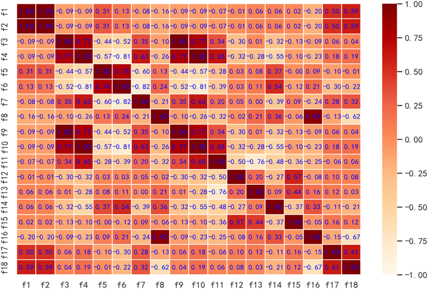
FIGURE 2. Correlation matrix of feature set.

The Figure 2 shows the degree of linear correlation between the extracted features. Among them, f1 and f2, f3 and f9, f4 and f10 are completely related, so f2, f9, and f10 are deleted, and the remaining 15 features are retained. Some features are still highly correlated, that is, these features contain more overlapping information. Through principal component analysis or factor analysis, new variables that are independent of each other can be constructed to eliminate the information overlap between the original variables. In this paper, 15 power consumption features are used for dimensionality reduction processing to obtain several new features. All new features are arranged in descending order according to the contribution rate. Table 2 intercepts the top seven new features with high contribution rate.

TABLE 2

TABLE 2. Contribution rate and cumulative contribution rate of new features after PCA dimensionality reduction.

When the number of new features reaches 5, the cumulative contribution rate of the PCA dimensionality reduction method reaches 98.24%. As can be seen from Section 3.2.2, five new features can well reveal the original feature information.

4.3 Result analysis

The k-means clustering algorithm is used to cluster the data set, and the optimal k value is determined according to the elbow method. It can be seen from Figure 3 that an inflection point occurs when k = 4, so the feature data set is divided into four categories.

FIGURE 3

FIGURE 3. Elbow method to determine k value.

Figure 3 shows the classification of the users according to the clustering results and count the number of each type of users. Among them, there are 124 users in category 1; 6,155 users in category 2; 153 users in category three; and 13 users in category 4. Due to space limitations, this paper only presents the anomaly detection process of the second type of users, and other types of users can be handled in the same way. The cluster center of a certain category reflects the overall characteristics of all samples in this category, so the power consumption curve of users in each category of cluster center can be used as the typical power consumption curve of the corresponding category, and the power consumption curve of typical users of different categories as shown in Figure 4.

FIGURE 4

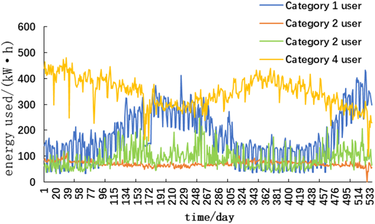
FIGURE 4. Power consumption curve of typical users of different categories.

The second type of user’s electricity consumption characteristic index is used as the input data of the abnormality detection algorithm in this paper, and the comprehensive abnormality score of each user is calculated, and it is used as a quantitative index of the abnormality degree of electricity consumption.

The ROC curve reflects the effectiveness of the algorithm. This paper compares the KNN algorithm, logistic regression algorithm, naive Bayes algorithm and the outlier detection effect of the algorithm in this paper. It can be seen from Figure 5 that the difference in AUC of the area under the ROC curve of the KNN algorithm and the logistic regression algorithm is small, while the AUC of the area under the ROC curve of the method in this paper is larger than that of the KNN algorithm, the logistic regression algorithm and the Naive Bayes algorithm which has a higher AUCdetection accuracy.

FIGURE 5

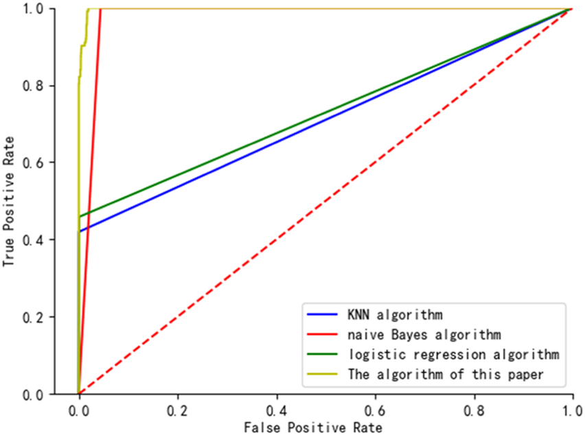
FIGURE 5. Comparison of ROC curves of the four algorithms.

Table 3 is a comparison table of the precision rate, recall rate, AUC value and F1 score value of each algorithm. Figure 6 more intuitively shows the difference between the accuracy and recall of the algorithm in this paper and other comparison algorithms. The precision rate of the KNN algorithm and the logistic regression algorithm and the recall rate of the Naive Bayes algorithm are slightly higher than electricity anomaly detection model based on entropy weight method and isolated forest algorithm, but the recall rate of the algorithm in this paper is slightly higher. The rate and F1 score are significantly higher than those of the KNN algorithm and the logistic regression algorithm, and the AUC values of the algorithm in this paper are higher than those of other algorithms. Considering the evaluation indicators of each algorithm comprehensively, the algorithm in this paper has a better anomaly detection effect.

TABLE 3

TABLE 3. Algorithm model performance comparison.

FIGURE 6

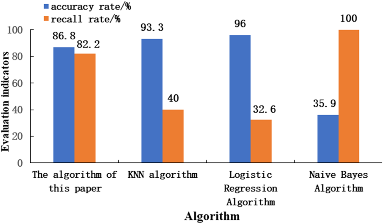
FIGURE 6. Comparison of indicator histograms.

5 Conclusion

Aiming at improving the efficiency of abnormal electricity consumption data detection, this paper proposes an abnormal electricity consumption detection method based on entropy weight method and isolated forest tree algorithm. Given that a large number of normal users perform various electricity consumption patterns, the model firstly classifies electricity users with different electricity consumption behaviors based on the k-means clustering algorithm; Secondly, the model calculates the weight coefficient of the indicator; Finally, the feature-weighted isolated forest algorithm is used to detect abnormal electricity users. The experimental comparison using the electricity consumption data of Irish residents to verify that electricity anomaly detection model based on entropy weight method and isolated forest algorithm has a higher precision and recall rate in a close to the actual detection environment.

Data availability statement

Publicly available datasets were analyzed in this study. This data can be found here: Previously reported electricity data was used to support this study and are available at https://www.ucd.ie/issda/data/commissionforenergyregulationcer.

Author contributions

WJ:Conceptualization, methodology, writing original draft. GC: Data curation, Writing original draft. LC:visualization and contributed to the discussion of the topic.

Funding

The authors declare that this study received funding from Jilin Lingzhan Technology Co., Ltd. The funder was not involved in the study design, collection, analysis, interpretation of data, the writing of this article or the decision to submit it for publication.

Conflict of interest

The authors declare that the research was conducted in the absence of any commercial or financial relationships that could be construed as a potential conflict of interest.

Publisher’s note

All claims expressed in this article are solely those of the authors and do not necessarily represent those of their affiliated organizations, or those of the publisher, the editors and the reviewers. Any product that may be evaluated in this article, or claim that may be made by its manufacturer, is not guaranteed or endorsed by the publisher.

References

Angelos, E. W. S., Saavedra, O. R., Cortés, O. A. C., and de Souza, A. N. (2011). Detection and identification of abnormalities in customer consumptions in power distribution systems. IEEE Trans. Power Deliv. 26 (4), 2436–2442. doi:10.1109/tpwrd.2011.2161621

CrossRef Full Text | Google Scholar

Cer (2011) Data from The commission for Energy regulation(CER)-smart-metering project[EB/OL].[2011-05-16] https://www.ucd.ie/issda/data/commissionforenergyregulationcer.

Google Scholar

Hu, Tianyu, Guo, Qinglai, and Sun, Hongbin (2019). Nontechnical loss detection based on stacked uncorrelating autoencoder and support vector machine. Automation Electr. Power Syst. 43 (1), 119–127.

Google Scholar

Huang, Y., and Xu, Q. (2021). Electricity theft detection based on stacked sparse denoising autoencoder. Int. J. Electr. Power & Energy Syst. 125, 106448. doi:10.1016/j.ijepes.2020.106448

CrossRef Full Text | Google Scholar

Hyvärinen, A., and Oja, E. (2000). Independent component analysis:algorithms and applications. Neural Netw. 13 (4-5), 411–430. doi:10.1016/s0893-6080(00)00026-5

PubMed Abstract | CrossRef Full Text | Google Scholar

Kim, M. S., Yang, H. J., Kim, S. H., and Cheah, W. P. (2007). Improved focused sampling for class imbalance problem. KIPS Transactions:PartB 14 (4), 287–294. doi:10.3745/kipstb.2007.14-b.4.287

CrossRef Full Text | Google Scholar

Li, Xinpeng, Gao, Xin, Yan, Bo, Chen, Chunxu, Chen, Bin, Li, Junliang, et al. (2019). Anomaly detection method of power dispatch flow data based on isolated forest algorithm. Power Grid Technol. 43 (04), 1447–1456. doi:10.13335/j.1000-3673.pst.2018.0765

CrossRef Full Text | Google Scholar

Liu, Guolong, Zhao, Junhua, Wen, Fushuan, Mao, Yiru, Wu, Zhanxin, and Xue, Yusheng (2020). A deep end-to-end super-resolution perception method for power distribution side load data. Automation Electr. Power Syst. 44 (24), 28–35. doi:10.7500/AEPS20200505018

CrossRef Full Text | Google Scholar

Monedero, I., Biscarri, F., León, C., Guerrero, J. I., Biscarri, J., and Millán, R. (2012). Detection of frauds and other non-technical losses in a power utility using Pearson coefficient, Bayesian networks and decision trees. Int. J. Electr. Power & Energy Syst. 34 (1), 90–98. doi:10.1016/j.ijepes.2011.09.009

CrossRef Full Text | Google Scholar

Mortaz, E. (2020). Imbalance accuracy metric for model selection in multi-class imbalance classification problems. Knowledge-Based Syst. 210, 106490. doi:10.1016/j.knosys.2020.106490

CrossRef Full Text | Google Scholar

Nizar, A. H., Dong, Z. Y., and Wang, Y. (2008). Power utility nontechnical loss analysis with extreme learning machine method. IEEE Trans. Power Syst. 23 (3), 946–955. doi:10.1109/tpwrs.2008.926431

CrossRef Full Text | Google Scholar

Rajendran, S., Meert, W., Lenders, V., and Pollin, S. (2019). Unsupervised wireless spectrum anomaly detection with interpretable features. IEEE Trans. Cogn. Commun. Netw. 5 (3), 637–647. doi:10.1109/TCCN.2019.2911524

CrossRef Full Text | Google Scholar

Song, Junying, He, Cong, Li, Xinran, Liu, Zhigang, Tang, Jie, and Zhong, Wei (2019). Daily load curve clustering method based on feature index dimension reduction and entropy weight method. Automation Electr. Power Syst. 43 (20), 65–72. doi:10.7500/AEPS20181115008

CrossRef Full Text | Google Scholar

Song, Xuankun, Han, Liu, Ju, Huangpei, Chen, Wei, Peng, Zhuyi, and Huang, Fei (2016). Review of China's smart grid technology development practice. Electr. Power Constr. 37 (7), 1–11. doi:10.3969/j.issn.1000-7229.2016.07.001

CrossRef Full Text | Google Scholar

Wold, S., Esbensen, K., and Geladi, P. (1987). Principal component analysis. Chemom. Intell. Lab. Syst. 2 (1), 37–52. doi:10.1016/0169-7439(87)80084-9

CrossRef Full Text | Google Scholar

Xu, Di, and Lu, Yuzin (2021). Identification of abnormal line loss for a distribution power network based on an isolation forest algorithm. Power Syst. Prot. Control 49 (16), 12–18. doi:10.19783/j.cnki.pspc.201267

CrossRef Full Text | Google Scholar

Xu, T. S., Chiang, H. D., Liu, G. Y., and Tan, C. W. (2015). Hierarchical K-means method for clustering large-scale advanced metering infrastructure data. IEEE Trans. Power Deliv. 32 (2), 609–616. doi:10.1109/tpwrd.2015.2479941

CrossRef Full Text | Google Scholar

Yu, Xuehao, and Zhao, Ziyan (2021). Multi-label text classification for power ICT custom service system based on binary relevance and gradient boosting decision tree. Automation Electr. Power Syst. 45 (11), 144–151. doi:10.7500/AEPS20200511001

CrossRef Full Text | Google Scholar

Zhang, Lei (2014). Outlier mining based on kernel local outlier factor. J. Shanghai Dianji Univ. 17 (3), 132–136+143. doi:10.3969/j.issn.2095-0020.2014.03.002

CrossRef Full Text | Google Scholar

Zhang, W., Dong, X., Li, H., Xu, J., and Wang, D. (2020). Unsupervised detection of abnormal electricity consumption behavior based on feature engineering. IEEE Access 8, 55483–55500. doi:10.1109/access.2020.2980079

CrossRef Full Text | Google Scholar

Zhang, Yao, Wang, Aohan, and Zhang, Hong (2021). A review of smart grid development in China. Power Syst. Prot. Control 49 (5), 180. doi:10.19783/j.cnki.pspc.200573

CrossRef Full Text | Google Scholar

Zheng, K. D., Chen, Q. X., Wang, Y., Kang, C., and Xia, Q. (2019). A novel combined data-driven approach for electricity theft detection. IEEE Trans. Ind. Inf. 15 (3), 1809–1819. doi:10.1109/tii.2018.2873814

CrossRef Full Text | Google Scholar

Zheng, Z. B., Yang, Y. T., Niu, X. D., Dai, H. N., and Zhou, Y. (2018). Wide and deep convolutional neural networks for electricity-theft detection to secure smart grids. IEEE Trans. Ind. Inf. 14 (4), 1606–1615. doi:10.1109/tii.2017.2785963

CrossRef Full Text | Google Scholar

Zhuang, Chijie, Zhang, Bin, and Hu, Jun (2016). Anomaly detection for power consumption patterns based on unsupervised learning. Proc. CSEE 36 (2), 379–387. doi:10.13334/j.0258-8013.pcsee.2016.02.008

CrossRef Full Text | Google Scholar