Review of corrosion monitoring and prognostics in offshore wind turbine structures: Current status and feasible approaches

1 Introduction

Offshore wind farm installations are becoming ever more popular. In the last decade, we have witnessed a steady increase in capacity of offshore wind farms and many countries (notably China and USA) have pledged to increase their capacity substantially in the future. In 2021, the newly installed capacity worldwide of offshore wind farms increased threefold with respect to 2020 (Lee and Zhao, 2022).

As a fast-growing renewable energy source, Offshore Wind Turbines (OWTs) benefit from two main advantages with respect to onshore wind turbines, namely: 1) higher mean wind speeds (modest increases in wind speed can result in doubling the generated power) and 2) steadier wind supply, which makes power generation more reliable. These two factors combined dramatically improve the return on investment (ROI) of such wind farms (Windpower Learning Centre, 2019).

While wind farms were initially installed mainly in coastal areas with shallow waters, nowadays offshore wind farms are increasingly deployed in deep waters (∼200 m depth) and further away from the shore (∼60 km) (Walsh, 2019; Keene, 2021). This leads to higher Capital Expenditure (CAPEX) and Operational & Maintenance (O&M) costs/Operational Expenditure (OPEX) (Castellà, 2020). In fact, O&M costs/OPEX may account for up to 30% of the Levelised Cost of Energy (LCoE) (May et al., 2015).

To reduce O&M costs/OPEX, advanced maintenance strategies like Condition-Based Maintenance (CBM) or Predictive Maintenance (PdM) need to be adopted to minimise the downtime (i.e., maximise the availability) of OWTs while performing all necessary maintenance actions. These advanced maintenance strategies require technologies such as sensing and monitoring systems, algorithms and software tools to process measured data for faults detection and remaining useful life (RUL) prediction, and software tools for decision making. Since the last decade, the development and deployment of such technologies to support the implementation of CBM/PdM strategy for onshore and offshore wind farms have been mainly focused on critical rotating components such as gearboxes, generators, blades, etc. (Crabtree, 2011; Kandukuri et al., 2016; Turnbull and Carroll, 2021). Different from the critical rotating components mentioned above, the current maintenance strategy typically employed for corrosion of wind turbine structures is time-based maintenance, where manual, on-site inspections by a maintenance team are carried out periodically (e.g., yearly), which significantly contributes towards the total O&M cost.

Since OWTs are exposed to harsh and corrosive environmental conditions, corrosion is a main root cause for offshore structure failure (Martinez-Luengo et al., 2016; Price and Figueira, 2017). Improper or degraded corrosion protection and inadequate management can result in structural degradation and even catastrophic failure. Therefore, it is vital for the implementation of CBM and PdM strategies to (also) cover corrosion of OWT structures.

In the literature, reviews can be found regarding diagnostics and prognostics of low-speed bearings and planetary gearboxes in wind turbines (Kandukuri et al., 2016) and regarding corrosion fatigue in OWT structures (Adedipe et al., 2016). In this paper we provide a review of the relatively new and increasingly important research area of diagnostics and prognostics of corrosion of OWT structures. While this topic is also considered in Abbas and Shafiee (2020), in this paper we mainly focus on evaluating and comparing various monitoring and prognosis techniques. To this end, we present an integral way the state-of-the-art of corrosion monitoring and prognosis solutions: from the understanding of the corrosion phenomenon and its modeling, to corrosion monitoring techniques and the use of the acquired data for corrosion prognosis, analysing the most suitable and cost-effective sensors and techniques for the application of OWT structures.

This paper is organised as follows. In Section 2 we give an overview of the corrosion mechanisms, corrosion protection techniques, and empirical models that describe corrosion loss over time. In Section 3 we consider corrosion monitoring techniques and systems, and their suitability for OWT structures. Then, in Section 4, we consider corrosion prognosis methods for the estimation of Remaining Useful Life (RUL) in the context of OWT structures. Moreover, we relate corrosion prognosis with maintenance strategies for O&M cost reduction. In Section 5, we analyse the most-suitable corrosion prognosis strategy intended for OWT structures. Finally, we provide a conclusion in Section 6.

2 Corrosion mechanisms and models

In this section, we first recall corrosion mechanisms and common corrosion protection systems. Later, we review a number of empirical corrosion models.

2.1 Corrosion mechanisms

One of the limiting states for the serviceability of Offshore Wind Turbines (OWTs), is corrosion that reduces structural integrity and durability of structural and non-structural components. The harshness of the offshore environment does not come as a surprise. Atmospheric corrosion in general accounts for more than half of the annual cost of global Gross domestic product (GDP)—which is estimated at approximately 3.8%—according to recent analysis of all types of corrosion (Chico et al., 2017; Hou et al., 2017; Koch, 2017). And as gas and oil installations have performed under such conditions for decades, much knowledge has been accumulated about the strict measures needed to be taken to mitigate corrosion before leading to catastrophic failures (Momber, 2011). In fact, the protection philosophy adopted for OWTs copies mostly the strategies implemented for gas and oil installations.

Today, the corrosion protection for OWT structures, and for the design basis, is well described in the design codes and semi-empirical correlations developed by certification authorities such as DNV and American Petroleum Institute (API). DNV is involved in 90% of all offshore wind farms worldwide as a certification provider. The relevant DNV Standards and Recommended practice documents that address the corrosion protection needed for OWTs regarding their structural integrity, can be found in DNV (DNV, 2014; DNV, 2021a; DNV, 2021b; DNV, 2021c; DNV, 2021d; DNV, 2021e; DNV, 2021f; DNV, 2021g).

The chosen corrosion protection system shall be applicable for the specified design and operating and survival temperatures of the support structures, according to DNV-RP-0363 (DNV, 2021a). Corrosion control includes, according to DNV-RP-0416 (DNV, 2021b), the following:

• Corrosion allowance (CA).

• Cathodic protection (CP).

• Corrosion protective coatings.

Corrosion protective coatings are made of metallic, inorganic or organic materials, applied to a metal’s surface, in this context is steel, to prevent corrosion. The coating systems employed for wind farm corrosion control have been developed during the last decades through valuable experience from the offshore oil and gas industry (Weinell et al., 2017). Although these coating systems may have passed qualification tests, many other factors are decisive on the performance and durability of the coatings. Erroneous application of the coating or the production of defects during the installation and servicing of the wind turbine, result in defects, failures or scratches, exposing the metal to sea water which causes corrosion. In addition, coatings also experience ageing and degradation with time, hence in areas where the bare steel is exposed, corrosion will commence. This is in particular a realistic scenario in the splash zone.

Indeed, experience indicates a shorter lifetime of coatings than the recommended 20 years of designed life for OWTs. According to DNV-RP-0416 (DNV, 2021b), the coating lifetime in the splash zone can be expected to be only 10 years for the NORSOK M-501 Coating system no. 7A intended for splash zone protection, although longer lifetimes have been achieved (Momber, 2011).

In the splash zone, the structure is intermittently exposed to seawater due to tide or waves, and thus the corrosivity of this zone is seen to be particularly harsh on the metals, even though coated. In addition, maintenance is not practical and in many cases omitted. Also, Cathodic Protection (CP) is not effective at all times for parts of this splash zone. CP is a technique to prevent corrosion of steel immersed in seawater by applying a protective cathodic current, either by sacrificial anodes or by an Impressed Current CP (ICCP). Today’s cathodic protection is well established through DNV-RP-B401 (DNV, 2021c) and estimated values for protection are chosen based on tabulated standard values. However, according to experiences gained in Norway and Denmark, several CP failures have been identified, resulting in corrosion allowance being consumed faster than expected (Osvoll, 2011; Weinell et al., 2017; Nøhr-Nielsen and Mathiesen, 2018).

Hence, Corrosion Allowance (CA) is an important corrosion control method together with applied current for cathodic protection. CA is an extra wall thickness that is added when designing the structure, to compensate for any reduction of the thickness by corrosion. For primary steel structures (structures where failure has significant consequences, such as a tower or flanges) the CA can be calculated from the specified corrosion rates in DNV-RP-0416 (DNV, 2021b, Section 7). The equation states:

$\text{CA}=V_{\mathit{corr}}\left(T_D-T_C\right)(1)$

where V_corr is the maximum expected corrosion rate, T_C is the expected useful design lifetime of the coating and T_D is the design lifetime of the structure.

Both the corrosion rate and the useful coating lifetime are heavily affected by the corrosivity of the environment, and it is acknowledged that it is critical to both understand what to expect, but also to document the actual corrosivity. Fatigue calculations for design of wind turbine support structures, are based on a steel wall thickness—defined as the critical wall thickness—equal to the nominal wall thickness of which half of the corrosion allowance is completely lost over the full service life without decommissioning phase, see DNV-ST-0126 (DNV, 2021f). A wall thickness smaller than the critical wall thickness can consequently lead to the appearance of catastrophic structural failures, depending on the design philosophy chosen, i.e., on the safety factors used for the fatigue design, see information in DNV-ST-0126 (DNV, 2021f). Therefore, for diagnosis and prognosis of wind turbine structural defects caused by corrosion, both the historical and the actual wall thickness are required, e.g., by in-situ thickness measurement and monitoring.

The corrosivity of the environment is defined in several standards. In ISO 9223 (ISO, 2012a), the atmospheric environments are classified into six atmospheric-corrosivity categories, C1 to C6, representing an increasing harshness of the environment when moving from dry salinity-free onshore conditions, to wet and salt-influenced offshore conditions. According to the standard, three environmental parameters are responsible for driving the corrosion process, namely: 1) the effect of time of wetness (TOW), 2) the sulphur dioxide concentration or deposition rate, and 3) the sodium chloride deposition rate. In addition, the standard ISO 12944–9 (ISO, 2018), also addresses various immersed conditions in the classes Im1 to Im4, and the extreme atmospheric conditions offshore, given as the CX corrosivity class.

For OWTs, two corrosivity classes—CX-offshore and Im2/Im4—must be taken in account when planning the corrosion protection strategy, according to ISO 12944–2 (ISO, 2017). CX includes offshore areas with high salinity for tidal, splash and atmospheric zones. Im2 is for the zones permanently submerged in seawater without cathodic protection, while Im4 are with cathodic protection (ISO, 2017; Masi et al., 2019). However, in the splash zone, these two conditions meet in a synergistic way. While below sea level the average corrosion rate is measured at 0.2 mm per year, in the splash zone and tidal zone, corrosion rates may be from 0.4 to 1.2 mm per year (Higgins and Foley, 2014).

Based on empirical and experimental data from literature reviews, it becomes clear that the most important environmental factors affecting the corrosion process of carbon steels under marine immersion conditions are sea water temperature, dissolved oxygen concentration and flow velocity (Guedes Soares et al., 2011). The variation in salinity in open-ocean surface is typically between 32 and 37.6 ppt. In this range, the corrosion of steel alloys that typically corrode uniformly—as carbon steels—is not seen to be significantly affected (Melchers, 2006; 2009), whereas changes in oxygen concentration and temperature are seen to be more critical. Indeed, temperature affects corrosion kinetics, oxygen concentration and diffusion (Sørensen et al., 2009). It has been observed that at a temperature of 25°C, the corrosion of carbon steel in sea water was nearly doubled when compared with the corrosion at 10°C (Guedes Soares et al., 2011). The concentration of the carbon content is not regarded as a factor in corrosion of steels immersed in seawater. In general it is therefore believed that whether the material is a high or low carbon steel, or similarly a low alloy steel, cast iron, or cold rolled mild steel, the measured corrosion rates are essentially the same—at a specific site—for all carbon steels immersed in seawater (Melchers, 2006; Guedes Soares et al., 2011).

In contrast, in offshore marine atmospheric conditions, the corrosion mechanism is initiated with the metallic surface becoming wet, and corrosion then propagates—under certain conditions at even higher rates—during the drying of the water layer before halting upon complete drying. The wet phase is ascribed either to a condensation process due to changes in temperatures, or due to the hygroscopic effect of surface contaminants like dust and salts (Koushik et al., 2021). However, also fog, rain and melting snow, contribute to the wetness. Eventually, the formation of droplets and a thin layer of electrolyte will take place (Simillion et al., 2014). The corrosion process will hence take place each time the metallic surface is wet, and the rate will be strongly influenced by several variables. An abundant literature has been published for prediction of corrosion rates from meteorological and pollution parameters (atmospheric conditions) (ISO, 2012a; b; Klinesmith et al., 2007).

In both atmospheric and immersed conditions, carbon steels mainly corrode uniformly, with a homogeneously distributed metal loss over the surface. However, localized corrosion may also develop on a surface initially corroding uniformly (Khodabux et al., 2020), explained due to effects from biological organisms in the sea water and the built-up of corrosion products. Non-uniform corrosion mechanisms happen when the electrochemical cell is distributed in an abnormal way over the surface of the metal, such that anodic and cathodic sites differ in size, resulting in an accelerated localized loss of metal and the formation of cavities and holes. Local differences with respect to oxygen access will cause differences in potential and pH and result in the initiation of localized accelerated cells, consistent with the theory of differential aeration corrosion (Melchers, 2013). Hence surfaces initially corroding uniformly, may develop non-uniform corrosion. Nonetheless, in order for crack growth to pose a threat to the structural integrity, the crack growth rate has to surpass the general corrosion rate. Otherwise, the crack geometry will be exfoliated and no fatigue crack growth will occur (Moghaddam et al., 2019). See Table 1 for information about the types of corrosion that are expected in the different corrosion zones.

TABLE 1

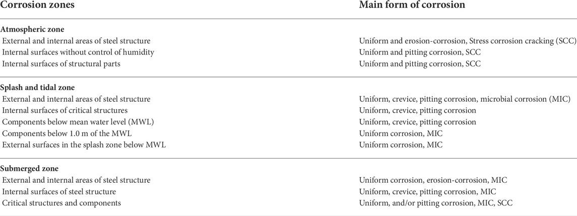
TABLE 1. Corrosion zones and form of corrosion in OWT. Adapted from (Price and Figueira, 2017).

To add to the complexity of predicting corrosion rates, bacteria life at the offshore site may cause marine growth on immersed structural components, while the highest is actually seen in the splash zone. This growth can affect not only the geometry, surface texture and the accessibility of the component, but also the corrosion rate when the coating on the steel structures has completely failed.

2.2 Corrosion models

The lifetime of a material, as described in the previous section, is highly dependent on its exposure to the environment. In the current state-of-the-art, lifetime and ageing assessment are performed by means of experiments, namely by combining 1) accelerated and 2) field testing. The limitation of the first testing method is that the conditions of the accelerated corrosion tests may not necessarily be representative for the real environmental conditions, or the degradation mechanisms happening in real life. The limitation of the second testing method is that it takes many years, about 10–20 years, to complete the test.

To model corrosion, the electrochemical process must be translated into mathematical equations—which require several simplifications and assumptions to be made. The major concern in making the correct assumptions is the multi-scale nature of corrosion and therefore the need of many model parameters that will limit the validity window of the model. In addition, many different environmental situations need to be taken into account by the models. The complexity of the model will thus be defined by the amount of parameters chosen to be included. For long time and length scales, empirical modelling may be suited as it is not computational expensive and presents valid solutions as long as changes in the corrosion mechanism can be excluded (Melchers, 2006; 2018).

Extensive overviews of the advances in atmospheric corrosion modeling can be found in Klinesmith et al. (2007); Morcillo et al. (2013); Simillion et al. (2014). In this section we review various empirical models for corrosion degradation highlighted in the literature. The majority of corrosion models for both immersed and atmospheric conditions, have been expressed as power-law models in the form of (Klinesmith et al., 2007; Simillion et al., 2014):

$M=K{t}^n(2)$

where M is the total accumulated corrosion at time t, t is the exposure time, K is the corrosion value of year one, while n is a mass loss component - usually less than unity. The latter represents the effects of all other factors that affect the corrosion process, including environmental conditions, and is usually estimated using a log-linear regression analysis of the measured data (Klinesmith et al., 2007).

Although these models incorporate the effect of exposure conditions, the corrosion loss is predicted as a function of time only. As a consequence, the variation related to environmental conditions, will only appear as error variations in these time-dependent models. A model for long-term exposure in atmospheric conditions that incorporates multiple environmental adjustment factors in addition to the time factor, is proposed in Klinesmith et al. (2007).

$y=c_1{t}^{c_2}{\left(\frac{\mathrm{T}\mathrm{O}\mathrm{W}}{c_3}\right)}^{c_4}{\left(1+\frac{\mathrm{C}\mathrm{l}}{c_5}\right)}^{c_6}{\left(1+\frac{{\mathrm{S}\mathrm{O}}_2}{c_8}\right)}^{c_9}{e}^{c_7\left(T-T_0\right)},(3)$

where y is the wall-thickness loss, t is the time duration, TOW is the fraction of time that the humidity is above a certain threshold value—which according to ISO 9223 is defined as the annual fraction of number of hours/year in which RH $>$ 80% and T > 0°C, SO₂ is the sulfur dioxide concentration, Cl is the chloride deposition rate, T the temperature in Kelvin, and c₁, … , c₉ are empirical constants. This formula represents the fact that while sulfur dioxide and chloride are catalysts for corrosion, humidity is required for corrosion. In the case of OWTs, the concentration of sulfur dioxide can be assumed to be zero, simplifying the equation above.

However, these most common approaches of modelling the loss of a metallic surface due to corrosion, have been significantly criticized in later years since the corrosion process is over-simplified taking into account only the oxidation of the steel produced by the arrival of oxygen to the corroding surface (Melchers, 2009). In general, data have been found to deviate from the relation described by Eqs. 2, 3, as it was observed that actual high initial corrosion rates would decrease gradually with increasing exposure time t, but later again would increase.

In Melchers (2018) the bi-modal model is proposed. This contains two modes, each described by a power law relationship. The first mode starts with a linear phase progressing to become a power law model, while the second mode starts with a power law model (with different parameters from in the first mode) to move towards a linear phase (with constant corrosion rate). In both modes, the power law is adapted by adding a phase with constant corrosion rate. The model explains the corrosion behaviour trend not only for atmospheric and submerged exposures, but also for tidal conditions. The model, although originally considered as “phenomenological”, attempts to explain the controlling processes at each stage of the corrosive mechanism as it develops with time. It addresses not only the oxygen reduction rate on steel, but also the effects on the corrosion rates by bio-films and corrosion products.

Figure 1 provides an overview of the bi-modal model. The two modes are distinguished by the parameter t_a. The first mode represents a short phase during which corrosion initiates, until the surface is covered by a rust layer at t_a, which retards the oxygen diffusion to the surface and decelerates the corrosion rate. The rate eventually stabilizes on a steady-state in the long-term.

FIGURE 1

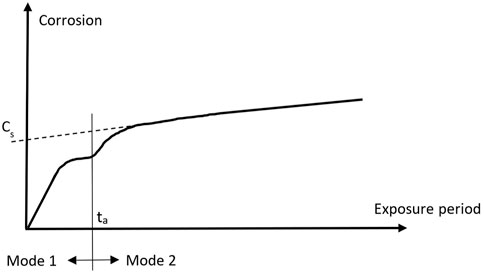
FIGURE 1. Melcher’s bi-modal model shown to be relevant for mild and low alloy steels as well as for chromium steels under various exposure conditions. Adapted from Melchers (2018).

The parameters t_a and c_s, along with other parameters in the model, have been estimated based on real-world data for coastal unpolluted sea-waters collected from various controlled experimental sources—showing that most corrosion damages occur within the first few years of exposure (Melchers, 2018).

However, existing models are to be regarded as incomplete, as they have been built based on quite simplified assumptions, without considering the dynamic change of the electrode geometry and effect of the consequent changes in the local environment—which are critical for locally accelerated corrosion. Some attempts have however been done the last years to model dynamic film variations, as well as the effect of corrosion products (Simillion et al., 2014; 2016; Gießgen et al., 2019).

2.3 Corrosion in offshore wind turbine structures

From the discussion in previous subsections, we found out that:

• Experiences from existing OWT farms suggest that coating lifetime is highly dependable both on the workmanship during the application of the coating and installation of the turbines, but as well on the corrosivity of the environment, acknowledged to be a critical factor also for the subsequent corrosion of the steel.

• Although carbon steels corrode mainly uniformly, and CP is applied on OWTs from the splash zone and down into immersed conditions, CP failures (due to unforeseen factors not covered by standards together with unfavourable conditions resulting in high localized corrosion rates) may lead to faster consumption rates of employed corrosion allowances.

• Corrosion models are necessary, together with input from real service corrosion rates, in order to mitigate risks for fatigue failures. We presented some well-known empirical corrosion models employed for uniform corrosion, and discussed how corrosion mechanisms may affect the expected corrosion rates. These models are essential for corrosion prognosis, discussed in Sections 4 and 5. In particular, the bi-modal model seems to describe well the corrosion behaviour in OWT structures.

3 Corrosion monitoring

As previously discussed in Section 2.1, inadequate corrosion management in offshore can lead to significant maintenance costs or even catastrophic corrosion failures. Therefore, a methodical and frequent corrosion inspection or continuous corrosion monitoring method has to be applied. Corrosion monitoring requires frequent unattended inspections, whereas corrosion inspection is carried out much less frequently with one inspection during a time period. For a corrosion prominent environment as offshore and possible situations where corrosion may not be detected before leakage, crack, or fatigue of the structure, it is important to have a systematic corrosion monitoring approach to detect the very slow progress of corrosion rather than an inspection routine.

This section is organised as follows. Section 3.1 presents sensors and techniques used for corrosion detection. In Section 3.2 Non-Destructive Testing (NDT) based corrosion monitoring and works found in literature for possible corrosion monitoring solutions are presented. Focusing on corrosion monitoring in Offshore Wind Turbines (OWTs), appropriate design parameters for a corrosion monitoring system, and challenges to be encountered are discussed in Sections 3.3 and 3.4 respectively.

3.1 Structural health monitoring sensors and techniques: Corrosion detection

Offshore O&M is a key discipline in structural health monitoring (Yang et al., 2018). In O&M tasks, it is important to detect material degradation due to corrosion phenomena which can be done by employing various types of sensors and techniques. Corrosion is detected by sensing different physical parameters based on their operating principle such as mass loss, corrosion currents, wall thickness changes, leak vibrations, surface discontinuities, cracks, or strain changes of the test material.

Corrosion measurements can be performed in several modes:

• Offline: a sample is taken for the testing process,

• In-line: install testing equipment with direct contact to the fluid of the corrosion process and retrieve the sensor probe for the analysis,

• Online: installation of testing probes in the field for continuous measurements of mass loss or corrosion rate directly from the system and no need to remove the test equipment to access the data,

• Online and real time: data from the online corrosion monitoring system can be accessed remotely. Literature distinguishes non-destructive and destructive methods for corrosion evaluation. Non-destructive testing (NDT) methods are evaluating the condition of the material without destroying the material or its properties, while in destructive testing, the tested item undergoes stress that eventually deforms or destroys the material.

The corrosion progress is observed by comparing the difference between measurements over some time duration (National Association of Corrosion Engineers, 1999; Kane, 2007). When the interval between consecutive measurements is large (e.g., months), the possibility of early detection of any corrosion becomes less probable. Therefore, continuous and frequent corrosion measurements give important information useful for early prevention and corrosion control actions.

3.1.1 Corrosion detection techniques and sensors

Corrosion sensors and corrosion detection techniques are key elements in corrosion management. Available types of sensors and related techniques for corrosion assessment are discussed next.

• Coupons for mass loss technique Corrosion can be monitored with the use of “probes” inserted and exposed to the corrosive environment for a specific time period. These corrosion probes can be either mechanical, electrical, or electrochemical. The conventional method for corrosion detection evaluates any weight loss based on the changes that happened to the test specimen geometry (Wright et al., 2019). The corrosion coupons are the probes used in this type of testing and have been widely used in the industry for many years. Coupons are made of the same material as the object being tested, with suitable weight and shape, and are exposed to the corrosion environment for a specific time period. The weight loss and data processing must be completed offline after withdrawing the coupons by trained staff (Kansara et al., 2018). Corrosion rate given in this method is an average value for specific exposed time duration and no real-time information is provided. The electrical version of the corrosion coupons are Electrical Resistance (ER) probes and they monitor corrosion in real-time using the electrical resistance parameter. The principle of this method is measuring the mass loss that happens in metallic probe/wire exposed to a corrosive environment based on the changes in electrical resistance due to corrosion products (Soh et al., 2016). The ER probes can provide online corrosion rate information using embedded devices with communication capabilities but the main drawbacks of ER probes are that they need exposure to the same environmental conditions of interest (e.g., same temperature, chemistry, flow regime), the probes have to be replaced frequently due to the weight loss they experience while immersed in the corrosive environment, and the sensitivity level depends on the probe design.

• Electrochemical sensors and techniques The corrosion process is mostly a natural electrochemical phenomenon. Hence, electrochemical sensors are used in corrosion detection by evaluating the electrochemical characteristics of the corroding material. The five most used electrochemical methods in corrosion detection are Open circuit potential (OCP), Linear polarized resistance (LPR), Galvanostatic pulse method, Resistivity method, and Electrochemical noise (EN). Electrochemical techniques (Holcomb et al., 2001) generally rely on measuring potentials and current densities with special electrodes introduced in the environment where corrosion monitoring is needed. The actual structure metal is not usually a part of the measurement circuit/setup. Their main advantage is that they can directly measure the corrosion rate and therefore continuous monitoring is possible. But these methods can alter the corrosion process and are considered an intrusive technique (Perkins, 2005). Furthermore, the type of electrodes compatible with the process must be carefully selected for each application to have enough sensitivity for corrosion measurements. Normally these solutions can not be left unattended for long periods of time in contact with the fluids that are producing the corrosion (National Association of Corrosion Engineers, 1999; Xia et al., 2021).

• Magnetic sensors and techniques If the test material shows some conductive properties, electromagnetic sensors can be used to detect corrosion by employing them in electromagnetic testing methods such as Magnetic Flux Leakage (MFL), Eddy Current (EC) method, Pulse eddy current method, and Magnetic Particle Inspection.Magnetic sensors measure magnetic flux or magnetic flux density changes. The oldest and most common magnetic sensors are known as detector coils or pickup coils which are a combination of excitation and receiver coils and used to detect corrosion based on magnetic flux changes across its coil. Their operation is based on Faraday’s law of induction. The sensitivity of these sensors depends on number of turns, permeability and section diameter (Watson, 2021). The transmitter coil of the sensor is excited with an alternating current to produce an alternating magnetic field which induces eddy currents in the surface of test material. The presence of defects or discontinuities in the surface/near-surface that are caused by corrosion can be inspected via the combined effect of the primary electromagnetic field with the secondary magnetic field from the eddy current. The changes that occur due to corrosion will induce a phase shift, magnitude changes in electrical conductivity, and magnetic permeability of the combined effect. This is known as the Eddy Current (EC) technique in non-destructive testing (García-Martín et al., 2011). In EC, the excitation signal is applied as a single frequency or sequence of signals with multi frequencies. Improving EC technique further, the pulsed eddy-current (PEC) technique has introduced with use of an excitation signal with a pulse of selected frequency and pulse width. PEC has potential to apply combination of multi-frequencies in the excitation pulse which have then the potential to inspect multiple depths simultaneously reducing the inspection time compared to EC (He et al., 2012; Sophian et al., 2017).In Roach and Nelson (2007) a novel electromagnetic sensor called Magnetic carpet probe (MCP) is presented. It is based on Remote Field Eddy Current (RFEC) and it is designed to be mounted as an in-situ application sensor. These sensors are made of flexible PCBs (Printed Circuit Boards) with highly dense printed coil. Corrosion is detected using the remote field eddy current technique. It has been observed that they are capable to generate a stronger magnetic field compared to conventional eddy current excitation. However, there is no evidence that the solution has been tested in a relevant environment. The aim of these tests was to evaluate the sensor performance during the development stage.SQUID (Superconducting quantum interference device) is another type of electromagnetic sensors designed to detect very low magnetic induction levels during eddy current testing. Though these sensors have very good sensitivity, their use is limited in many corrosion detection applications as they need highly controlled conditions to operate (e.g., temperature) (Bellingham et al., 1987).Hall effect sensors are widely used types of electromagnetic sensors to detect the presence and magnitude of a magnetic field. These sensors are operating based on the hall effect produced by sensing the magnetic flux. Based on its operating principle, these sensors are used to detect the flux leakage of Magnetic Flux Leakage (MFL) NDT method. In the MFL method, the testing conductive material is magnetized by applying a magnetic field, and the leaked magnetic field lines out of the material surface due to the presence of any defect is detected and converted into an electrical signal by hall effect sensors (Shi Y. et al., 2015; Shams et al., 2018). Magneto-resistive sensors are another type of electromagnetic sensor used to detect flux leakage in MFL technique. Their operation is based on the magneto-resistance property which exhibits a linear change in the resistance of its material under an external magnetic field (Jander et al., 2005). These sensors are capable of detecting low-frequency and multi-frequency eddy currents during electromagnetic material testing. While these sensors are highly sensitive and accurate, they have a high-temperature coefficient (García-Martín et al., 2011).The advantages of these electromagnetic sensors and techniques (EC and MFL) are the tests can be performed without contact, can measure through coatings and insulating materials, and is suitable for outdoor operations. Limitations with magnetic sensors and techniques are that test material needs to be conductive, depth of penetration is limited (inspection is limited to surface or near-surface), the results depend on the electromagnetic properties of the test material, the sensibility and resolution of the measurements are very dependent on the distance between the excitation coils, and the test material (Hernandez-Valle et al., 2014; Shi Y. et al., 2015; Sophian et al., 2017) and the results can be affected by other electromagnetic fields.

• Acoustic sensors and techniques One of the most popular non-destructive types of corrosion detection sensors is acoustic sensors, which are capable of evaluating the material’s mass and changes in geometry. The most common type of acoustic sensor is a piezoelectric sensor/transducer. Piezoelectric sensors are capable of measuring vibrations in the form of force, stress/strain, pressure, temperature, or acoustic emission, and converting them into a measurable electric signal. The most significant characteristic of these sensors is that they can convert mechanical energy into electrical energy and, conversely, electrical energy into mechanical energy (Taheri, 2019). They are capable of generating high-frequency acoustic waves using an excitation electric pulse/pulses and evaluating a material through its mechanical vibrations (Wright et al., 2019). In ultrasound (US) corrosion detection technique, a high-frequency sound wave is generated using a piezoelectric sensor and transmitted through the test material to evaluate any discontinuities or thickness loss. The time difference between the reference signal and the transmitted or reflected part of the signal (based on different acoustic impedance) is converted into a defect/thickness loss (Kansara et al., 2018; Herraiz et al., 2019; Thibbotuwa et al., 2022). The advantages of the US technique are that tests can be performed fast and accurately, and inspection is possible for higher thicknesses in both conductive and non-conductive objects. The major limitation is that small or thin materials are difficult to test, and it is very sensitive to the quality of the contact between the piezoelectric sensor and the test material.In US method, contact is needed between the test piece and sensor. To overcome this constraint, there are few methods based on non-contact acoustic wave generation in a test material, such as electromagnetic acoustic transducers EMATs (Electromagnetic Acoustic Testing), air (gas) coupled systems, and optical interferometric detection (Green Jr, 2004). Among them, use of EMAT transducers are a quite popular method that generates acoustic waves with no contact using electromagnetic induction. They consist of two major components: a magnet to generate a low frequency or static magnetic field and an electric coil with alternating current to generate a relatively high-frequency field. Interaction of these two magnetic fields will generate a Lorentz force and obtain a mechanical vibration in the solid lattice creating an ultrasound wave. However, in comparison with piezoelectric transducers, the EMAT transducers have lower efficiency during energy conversion, and the size of the transducer is relatively large because it consists of bulky and powerful magnets or electromagnets (Green Jr, 2004; Hernandez-Valle et al., 2014).Acoustic Emission (AE) is a non-destructive material testing method based on detecting the transient elastic waves in a sudden redistribution of stress in a material (Faisal et al., 2017; Yue et al., 2021). Energy released by AE localized sources (e.g., crack, slip or dislocation movements, or phase transformations in metals) propagates through test material which is received by the AE sensor. The conventional AE sensors are made of piezoelectric material that are generally sensitive to exciting frequencies between 20 and 400 kHz (Vallen Systeme GmbH, 2017). With the aim of improving the signal-to-noise ratio of conventional piezoelectric AE sensors, Micro-Electro Mechanical Systems (MEMS) acoustic emission sensors have been developed. Moreover, they have significant reduced size and weight compared to conventional AE sensors (Ozevin, 2020). The AE technique has potential to quantify cracks and leaks, but have limitations in the response depending on the source intensity/energy released. Moreover, it offers limited repeatability of measurements, only detects active/growing defects, and the presence of noise limits the sensitivity considerably.

• Thermography Thermal cameras are sensing devices used to measure the rate of heat emission of surfaces emitted by objects. Imaging with a wavelength in the infrared range (0.7–300 microns wavelength) is known as Infrared (IR) Thermography (TH). IR cameras sense the IR radiation emitting from a test object (Jönsson et al., 2010). Both thermal and IR cameras are employed to detect corrosion in two possible ways: passive and active. In the passive method, thermal energy or IR radiation emitted by the inspecting surface/object is monitored, and in the active method, additionally an external source is used to stimulate the heat flow inside the object (Theodorakeas et al., 2015). As heat diffuses through the structure, the measured temperature distribution gives information about defects or thickness (Grinzato and Vavilov, 1998). Recent literature shows that based on the way of heat stimulation, this can be categorized as optical thermography (Jönsson et al., 2010; Doshvarpassand et al., 2019), induction thermography (Cadelano et al., 2016; Tian et al., 2016), vibration thermography (Doshvarpassand et al., 2019), microwave thermography (Foudazi et al., 2015), and laser thermography (Hwang et al., 2019).

• Radio frequency identification sensors (RFID sensors) Radio-Frequency Identification (RFID) sensors are another sensor type which have been used for structural health monitoring and can be used for corrosion detection. Typical way of corrosion detection based on RFID sensors consists of shielding RFID tags (transponders) with corrosion sensitive element and evaluates how the communication response characteristics sensed between RFID tags and receiver is affected when the corrosion takes place (He et al., 2014; Zhang et al., 2016). However, even though this technology can provide cost effective solutions for corrosion detection, it can only be used for atmospheric corrosion, not to evaluate the corrosion condition of the structure itself.

• Radiography (RT) is a type of volumetric inspection technique based on the effects of X-Ray passing through the specimen and producing a radiograph. This technique most commonly has been used for pipe inspection (Zscherpel et al., 2006). X-ray generators producing the beam (Hanke et al., 2008), display devices and collimators to direct radiation beam to the place of inspection (Jensen and Gray, 1992) are the devices that are occupied during the inspection process.

• Visual Inspection Visual inspection is a common and widely used corrosion inspection method in many applications. Assessment of corrosion condition of the structure is done by visual appearance and this can be executed without any complex tools and equipment when there is physical access to the object. This method has been enhanced using cameras to capture the structure with images or video during the inspection followed by various advanced image processing techniques enhancing the feature classification and segmentation process for better efficiency. However, visual inspection is challenging and ineffective when it is difficult to access the target structure. As well, not appropriate when a quantitative assessment of corrosion is required.

Additionally, integrating corrosion detection sensors/methodologies to Unmanned Aerial Vehicles (UAVs) or remotely piloted aircraft have become a very promising approach for providing remote access during structural health inspection activities. This is important because integrating UAVs with an inspection system of NDT sensors can facilitate to perform measurements in different locations of the structure using the same sensor. Mainly, UAVs have been used in visual inspection methods with embedded high resolution cameras allowing remote visual inspection of the structures Shafiee et al. (2021).

To summarize, corrosion detection sensors and technologies are available based on different sensing principles evaluating different physical variables. Each of these technologies has its own advantages and technical limitations making their use beneficial or limited in certain applications.

3.2 Corrosion monitoring based on non-destructive testing

The degree of complexity of a corrosion monitoring system is illustrated in Figure 2 based on the technical capacity of each corrosion sensor/detection method, and different levels of system implementations. When the level of implementation increases, the capabilities of the corrosion monitoring system also increase.

FIGURE 2

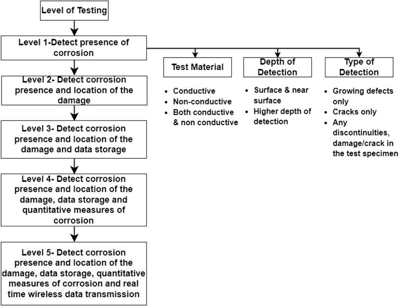
FIGURE 2. Levels of complexity in corrosion monitoring systems.

NDT methods are more appropriate for corrosion monitoring systems, as they are expected to operate with minimum human interventions for long time in the field. Among the methods discussed in Section 3.1, all the magnetic techniques, acoustic techniques, thermography, and RFID are considered as non-destructive and non-intrusive techniques (Forsyth, 2011; Khan et al., 2020; Márquez and Chacón, 2020). On the other hand, electrochemical techniques (e.g., OPC, LPR, and EN) provide direct measurements of the corrosion process and can be used to determine real-time corrosion rates. However, electrochemical techniques are considered to be intrusive, which can alter the corrosion process itself. And sensor has to be in direct contact with the corroded area making them not very attractive if one plans to cover large areas for monitoring. In the case of RFID technique, the precision that can be obtained based on the degradation of the RFID signal is very poor. As in the case of electrochemical techniques, the RFID technique is not measuring the structure itself. In applications such as concrete structures, the RFID tag must be embedded in the target structure making the system more complicated during the installation and impossible to repair after deployment.

The chosen corrosion monitoring technique shall be non destructive, non-intrusive, and able to produce corrosion related quantitative measures. In addition, the application to be used, type of corrosion intend to detect, relevant environmental conditions, cost, properties of the material to be tested, coating types, and frequency of testing to be performed also have to be considered.

3.2.1 Corrosion monitoring systems and designs

As presented in Figure 2, the corrosion monitoring solutions can be in different testing levels. This is because, some are focused on methodologies to optimize the sensor characteristics and its performance but they are not ready as a complete deployed system. And some works present final solutions yet they are under or have not been in validation phase in relevant environments. In each of these cases, the works found in the literature with possible corrosion monitoring solutions/designs are discussed below.

In Zhang et al. (2017), a magnetic-based corrosion detection system has been developed to investigate the relation between corrosion rate and magnetic induction in steel reinforcement. In the system, a magnetic field is created using series-wound permanent magnets and the changes that happen in the magnetic induction due to substantial permeability difference between rust and steel is detected with a hall effect sensor. The results show that the mass loss in reinforced steel due to corrosion and the voltage increment of the hall effect sensor are linear and therefore it is concluded that the proposed magnetic corrosion device is capable of quantitative analysis of corrosion rate. In Wasif et al. (2022), authors propose magnetic eddy current based sensor for corrosion monitoring of pipelines. The sensor design optimization, sensitivity and power consumption have been studied. Moreover, the sensor was tested using as accelerated corrosion test on mild steel.

In Jiang et al. (2017), a stress wave based active sensing corrosion monitoring approach is presented using embedded piezo ceramic transducers for prestressed concrete structures. The proposed system would give corrosion information about two stages such as free expansion of the corrosion products and corrosion induced cracks occurrence quantifying the energy of the received signal based on Wavelet packet-based energy analysis. The proposed sensor dimensions are (25 mm × 25 mm × 25 mm) and it has been tested on two concrete beams (prestress and without prestress) under accelerated corrosion environment.

Although the solutions based on electrochemical sensors seem not to be the most suitable ones for corrosion monitoring, some approaches have been found in the literature. In Pei et al. (2021) authors propose galvanic cell type sensors able to achieve a quantitative corrosion evaluation when atmospheric corrosion occurs. However, these sensors are measuring the corrosivity of the atmosphere and it can only relate to the corrosion condition of a structure exposed in the same environment, but not evaluating the structure itself directly. In Figueira (2017), it is concluded that if electrochemical sensors are correctly employed for the corrosion monitoring of reinforced concrete, fast, reliable, and quantitative corrosion information can be obtained. In Leon-Salas and Halmen (2015) authors rely on electrochemical techniques as well. In this case, they proposed linear polarization and open circuit potential for the proposed corrosion monitoring system in reinforced concrete. The authors use RFID communications to send the data to a RFID reader acting as a datalogger. Although the provided results were obtained by placing the sensor on the steel bar, actually the sensor is supposed to be installed in structures before concrete is poured. This can be a constraint for a long term operation of the sensor because if any fault occur, there is no way of repairing or replacing these sensors. On top of that, long term performance testing of the proposed sensor in a real environment must be done in the future.

Project iWindCr (Ahuir-Torres et al., 2019) is an effort to find benchmarking parameters that can show early signs of corrosion in offshore. This approach is based on several types of electrochemical sensors providing data about the advancement of corrosion in specific locations of the wind turbine. Although the data obtained are mainly based on a pilot of the system and no conclusions can be drawn from the results given, the iWindCr system shows an interesting and relevant methodological approach to the problem of remotely monitoring corrosion of OWT structures.

In view of any breakdown in the applied coating will lead to the onset of corrosion, visual detection of such situations can be identified as critical corrosion points in a structure. These systems can serve as warning systems to detect the locations with possible risks, and could use with other complementary NDT methods to evaluate the structure condition quantitatively if needed. Such system has been proposed in Momber et al. (2022) as a condition monitoring approach based on automatic image acquisition and image processing for monitoring and maintenance planning of surface protection systems in onshore wind turbines.

Several interesting works have been presented related to integrating/thermal/IR cameras, sensors, and other required electronics circuitry with UAVs for corrosion detection. In particular, Liu et al. (2018) proposes a micro aerial vehicle (MAV) facilitated coating assessment system based on infrared active thermography with artificial intelligence (AI). However, the system work as an inspection system operated semi-autonomously. Working towards autonomous inspection, Andersen et al. (2020) investigate several deep learning architectures to find out the best suited for an autonomous inspection system. These architectures were investigated for marine corrosion classification where the inspection activities are proposed to perform by an UAV. However, the performance of the algorithms has not been evaluated in real-time and the results do not provide enough information about the location where corrosion is present and any quantitative measurement of corrosion.

A low power, low cost corrosion monitoring system based on ultrasound time of flight technology is implemented for OWTs (Thibbotuwa et al., 2022). The proposed system measures corrosion in the wind turbine tower (splash and atmospheric zones) and has the advantage of operating from clean side of the wind turbine, making it more appropriate for operation in marine environment. The system successfully provides thickness measurements in both bare steel and coated samples, and the precision of these measurements (around 1 μm) allows to achieve an intra-day estimation of the corrosion rate in real-time.

3.3 Corrosion monitoring in offshore wind turbine

Our definition for corrosion monitoring system is a reliable system which operates successfully unattended and is able to produce quantitative corrosion measures. In general, implementing a corrosion monitoring system with these requirements is challenging for any application field.

Based on the literature, we could not find any commercialized or automated system beyond the testing phase (in development stage) which is currently applied in real-time for corrosion monitoring in offshore wind farms in the way we defined above.

Considering the performance expectations of a corrosion monitoring system, the important factors for offshore are:

• The corrosion monitoring solution has to be able to operate long-term in the marine harsh environment (high level of salinity, humidity and in the presence of metallic objects and Electromagnetic Fields) successfully and provide reliable results with minimum interventions.

• Most essentially, corrosion monitoring technique, sensor, and sensor placements have to be decided according to the zone (splash zone, atmospheric zone, and submerged zone) or the part (nacelle, blades or tower) of interest to be monitored in the turbine and compatible with coating type or corrosion protection methods applied.

• Intended monitoring parameters: physical variable for corrosion detection and other parameters such as humidity, temperature, etc.

• How the selected technology is reflecting the actual corrosion condition and able to produce quantitative corrosion values.

• Accuracy and reliability of the measures.

• Sampling frequency.

• Able to develop as a real-time and cost-effective monitoring system which can provide data/information faster, better and user friendly.

• Easy to deploy and operate low power and unattended.

• The properties and characteristics of the corrosion sensor need to be assessed according to working temperature capacity, cost, power consumption, and accuracy level (Leon-Salas et al., 2011; Taheri, 2019).

In Table 2, the potential techniques to be used for corrosion monitoring in offshore, considering the above discussed factors, are evaluated. The performance indicators presented in the table for the evaluation of each technique are further clarified in below.

• Producing quantitative corrosion measurements implies the possibility of producing quantitative measures of corrosion involving simple/complex signal processing or either a few/more computational steps.

• Measurements rate indicates how frequently consecutive measures can be performed.

• Easy to deploy indicates that all the required components to perform the measurements can be deployed easily in the target field of operation.

• Contact need indicates that the sensor needs to be in contact with the surface.

• Through coating corrosion detection means that the technique can be used for corrosion monitoring in structures protected by coating.

• Depth of inspection is related to the possible depth of inspection that could be measured perpendicular to the sensor placement.

• Precise corrosion measures get better repeatability of the measurements and consequently, permit to predict the corrosion rate more precisely.

• Affected by electromagnetic fields implies that the obtained corrosion measurements can be affected/distorted by the presence of other electromagnetic fields.

• Measuring from clean side means that the sensor can be placed on the clean side of the structure to perform the measurements avoiding the side where corrosion progresses faster.

TABLE 2

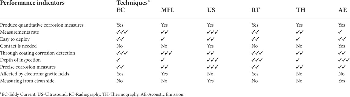
TABLE 2. Comparative study of feasible NDT methods for corrosion monitoring in offshore wind.

Taking all the requirements and the OWT use case into account, the ultrasound (US) technique seems a very promising candidate for the design of a corrosion monitoring solution as is shown in Table 2:

• It permits frequent and accurate measurements to increase the accuracy of corrosion prognosis estimates.

• It is easy to deploy, thereby reducing installation costs and risks.

• It is not affected by electromagnetic fields, which are present in the wind turbines.

• It is possible to measure from the clean side of the structure, which is key for a continuous monitoring system with the aim of protecting the electronics from harsh environments.

3.4 Challenges in corrosion monitoring in offshore

Research and development of corrosion monitoring systems in offshore have to encounter a number of challenges.

Almost every structure in any kind of application is corrosion protected by various types of coating layers. Early marine corrosion under coating is difficult to detect and determine the size of the defect with visual testing methods and it could be also challenging for other NDT techniques as well depending on type and thickness of the protective coating applied. From the corrosion detection and monitoring perspective, each layer of coating introduces a challenge. Another major challenge is obtaining accurate and reliable quantitative measurements of corrosion for long term (Martinez-Luengo et al., 2016). As discussed in Subsection 3.1.1 and Table 2, each corrosion detection technique has operational limitations. In particular, temperature may influence sensor readings and accuracy of most of the corrosion monitoring methods (Rommetveit et al., 2010). Therefore, corrosion measurements may need calibration based on temperature to obtain a better corrosion estimate.

Moreover, working on corrosion monitoring systems to optimize their performances and operate fully unattended could possibly add challenges such as incorporating them with wireless communication technologies for sending sensor data to a base station wirelessly, size and weight optimization of the overall solution, low power operation and maintain corrosion system production at low cost.

4 Corrosion prognostics

In the previous section we considered corrosion monitoring to determine the current state of corrosion. For scheduling maintenance or decommissioning, it is important to estimate the future corrosive state and in particular the Remaining Useful Life (RUL) of the Offshore Wind Turbine (OWT) structure. A (lifetime) prognosis method for a system estimates its RUL, or, more generally, the future trajectory of states of a system over time from the current state to its End Of Life (EOL). We can distinguish three types of prognosis methods: data-driven, model-based, and hybrid methods (An et al., 2015; Vachtsevanos, 2020), and below we give a brief overview of these types of prognosis methods. The types of prognosis methods that are most appropriate for a given problem are highly dependent on the type and the amount of data available and on the existence of accurate degradation models. We also discuss the applicability of the various prognosis method types for corrosion prognosis in OWT structures. For other failure modes of wind turbine structures we refer to Jardine et al. (2006) for a review on diagnosis and prognosis of mechanical systems.

4.1 Data-driven prognosis methods

A prognosis method is called data-driven if it uses only measurement data of the system under consideration and historical measurement data (measurement data with the corresponding RUL) of other similar systems. In particular, no model of the physical state of the system is used. Various data-driven prognosis methods exist, of which neural networks and Gaussian process regression are most often used (An et al., 2015).

4.1.1 Neural networks

An artificial neural network (simply called neural network) needs to be trained in order to learn a certain function f (i.e., a set of input-output pairs) up to some small error. A weight between every two connected neurons is used to linearly transform the output signal of a neuron before it is received by the next neuron, and training is used to alter the weights of the neural network to minimize the discrepancy with f. Activation functions associated to neurons are in turn a source of non-linearity to extend the expressivity of neural networks outside of the domain of linear functions. The chosen network topology and the amount of training data are crucial to learn f up to a small error. For a more detailed account of neural networks, we refer to the many standard treatments of this vast research area (Hagan et al., 2014; Aggarwal, 2018).

Neural networks have been used for corrosion prediction in various ways. For example, they have been used to predict corrosion polarization curves and corrosion rates based on both impedance measurements and historical data, respectively, see Kamrunnahar and Urquidi-Macdonald (2010). Also, corrosion rates have been predicted using neural networks based on meteorological data as input (Kenny et al., 2009). Moreover, corrosion depth has been estimated by neural networks using a database of published corrosion measurements as input (Cai et al., 1999). Neural networks have also been trained to estimate the pitting potential of stainless steel as a function of temperature and concentrations of salt, sulphate, carbonate, nitrate, and hydroxide (Cottis et al., 1999).

4.1.2 Gaussian process regression

Gaussian process regression is another data-driven method that can be used for prognosis. Recall that a Gaussian stochastic process is a natural generalization of the notion multivariate normal distribution to function spaces on a possibly infinite domain T. Now, Gaussian process regression (GPR) is a method to determine an optimal Gaussian stochastic process given a dataset and a covariance matrix k_t,t′ for t, t′ ∈ T that represents the similarity between elements of T (Rasmussen and Williams, 2006). For example, if T is a time domain, then the closer the points t and t′ are in time (i.e., the smaller |t − t′|), the larger their covariance. The output of Gaussian process regression is a Gaussian stochastic process for which functions f: T → D that are more likely to represent the ground truth, obtain a higher probability. In this way, a Gaussian stochastic process does not only give the most likely value for every t ∈ T (i.e., the mean of the random variable X(t)), but also its variance.

There are various papers in the literature that use GPR to estimate corrosion growth. GPR can be used to filter noisy measurements or to filter other outside influences. For example, GPR is used in Woo et al. (2020) to remove temperature effects on the estimation of corrosion potential. Also, GPR is used to predict a spatial map of wall thicknesses based on measurements of a number of spatial locations (Shi L. et al., 2015).

While applying GPR on corrosion process parameters for the sample under consideration is suitable for interpolation of the ground truth, this is less suitable for prognosis (i.e., extrapolation) as the uncertainty increases too quickly for many real-world applications. Therefore, in order to obtain reliable long term extrapolation, GPR needs to be applied to both the measurements of the current sample and historical measurement data of similar samples. Alternatively, GPR can be augmented with a physics-based degradation model (see Section 4.2) to obtain a hybrid solution, where GPR is used to estimate the parameters of the degradation model (for example, to estimate the corrosion rate (Liu et al., 2017)).

A natural generalization of Gaussian process regression is to consider stochastic process regression where the random variables X(t) satisfy possibly non-Gaussian probability distributions. Indeed, since corrosion depth cannot be negative it is natural to consider probability distributions for which negative values have probability zero. For example, the inverse Gaussian probability distribution satisfies this property while being similar to a normal distribution for non-negative values. In Zhang et al. (2013) inverse Gaussian process regression is used to estimate the wall thickness loss due to corrosion of underground energy pipelines. The parameters of this model were estimated by using measurement data from inspections.

For a (purely) data-driven prognosis method to be accurate, a large amount of both 1) measurements of the current corrosion sample and 2) historical measurement data of similar samples are needed. Therefore, the measurement data is typically sensor data that is acquired in an automated way. Moreover, the historical measurement data should be representative for the current measurements to give accurate estimates. Indeed, if the current measurement campaign is very different from any of the historical measurement campaigns, then the RUL estimate that is inferred by the prognosis method is likely too inaccurate.

Currently, there is very little historical corrosion measurement data available of walls of OWTs. Moreover, only very few OWTs have reached their EOL, so there is virtually no measurement data available of OWTs that are near their EOL. Consequently, given the above constraints on the applicability of data-driven prognostics, data-driven methods are currently not applicable for estimating the RUL of OWTs.

4.2 Model-based prognosis methods

A prognosis method is called model-based if the method uses an explicit model of the state of the system. The model may be based on first principles or based on empirical evidence. In case the model describes the degradation process of an asset, the model is called a degradation model. An example of a degradation model is a corrosion model. We may distinguish two types of model-based prognosis methods.

A first-principle prognosis method is a model-based prognosis method where the model of the state of the system is based on established laws of physics and empirical prognosis methods. An example of a first-principle prognosis method is the Paris’ law (Paris et al., 1961), which is a degradation model describing the growth of a crack in a material due to fatigue.

An empirical prognosis method is a model-based prognosis method where the model of the state of the system over time is based on observed trends in historical measurement data. By historical measurement data we mean here measurement data that was acquired from systems other than the system under consideration (i.e., from the system of which you would like to predict the RUL). We refer to Section 4.3 for prognosis methods that also use measurement data of the system under consideration. While the empirically obtained model gives a general trend, it typically has empirical constants. Regression methods like least squares are able to estimate unknown empirical constants based on historical measurement data of systems close to the system under consideration (An et al., 2015; Vachtsevanos, 2020). In Galea et al. (2009), corrosion prognostics for aircraft is considered where model fitting is historical data is followed by model extrapolation.

Model-based prognosis methods are accurate if the model, including the values of the empirical constants, accurately reflects reality. This implies that the physical degradation process is highly deterministic. Indeed, the (deterministic) degradation model cannot accurately reflect reality if there are several significantly different degradation trajectories possible. Even if the physical degradation process is highly deterministic and there is a well understood degradation model in place, it might be difficult to estimate the empirical constants of the model, in particular when there is little historical data available from systems similar to the one under consideration.

In the case of prognosis of wall thickness reduction due to corrosion in OWT structures, the physical degradation process is rather non-deterministic. Indeed, unexpected weak spots (that are not accounted for in the model) or accidental scratches in the coating surface can lead to a much earlier than expected onset of corrosion of the steel. Also, non-deterministic environmental influences, like weather and waves, are able to influence the corrosion process significantly. Finally, due to the lack of historical measurement data, the empirical constants can be only roughly estimated.

4.3 Hybrid prognosis methods

An hybrid prognosis method is a model-based prognosis method where measurement data of the system under consideration is used to improve the estimation of the current state of the system. The degradation model is then used to extrapolate future states based on the estimation of the current state. Consequently, a better estimation of the current state results in improved prognosis accuracy.

Essentially, a hybrid prognosis method provides a solution to the Bayesian filtering problem, which we discuss in Section 5.1, by estimating the most likely current state given the current measurement and the prediction of the model given previous measurements. See Figure 3 for an illustration of this approach. If certain empirical constants of the model are not precisely known, then a hybrid prognosis method is able to use the incoming measurement data to provide a better estimate of these constants. In this way, regression methods like least squares (mentioned in Section 4.2) that estimate unknown empirical constants can be used in hybrid prognosis methods to provide initial estimates of these constants, that are subsequently iteratively refined by filtering methods based on incoming measurements.

FIGURE 3

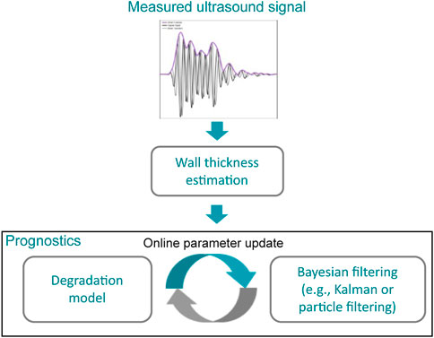
FIGURE 3. High-level overview of hybrid prognosis methods applied to the problem of corrosion prognosis using ultrasound.

An example of such a hybrid prognosis method applied for corrosion prognostics is given in Chookah et al. (2011). There, historical data is used to accurately estimate the two constants of an empirical model for corrosion-fatigue crack growth, and incoming measurement data is used to continuously improve this estimate through an approach similar to particle filtering (particle filtering is discussed in Section 5.3).

Using a hybrid prognosis method, a degradation model can adapt to incoming measurement data and “choose” the appropriate trajectory of a degradation model to deal with non-deterministic behaviour. Moreover, it can deal with initial rough estimates of empirical constants by iteratively adapting these constants to incoming measurement data.

4.4 Applicability of prognosis methods in offshore wind turbine structures

Regarding corrosion prognosis in OWT structures:

• Data-driven methods are currently not applicable for estimating the RUL of OWT structures due to the lack of sufficient amounts of historical corrosion measurement data (specially from OWT that have already reached their EOL).

• Model-based methods require model parameters that accurately reflect reality, which in the case of corrosion is difficult due to its rather non-deterministic nature. Besides, in OWT structures, the estimation of such parameters is difficult due to the lack of historical corrosion measurement data.

• In Hybrid methods, the degradation model can adapt to incoming measurement data, allowing to deal with the non-deterministic nature of corrosion. Besides, the iterative adaptation of model parameters allows for initial rough estimates which may be obtained with a limited amount of historical corrosion measurements.

Due to the above-described limitations of the data-driven and model-based approaches, the most suitable type of prognosis method for corrosion prognosis in OWTs seems to be hybrid prognosis methods. Consequently, an approach to corrosion prognosis using this type of method will be detailed in the remainder of the paper.

5 Prognosis method for corrosion of offshore wind turbines

Based on the types of prognosis methods discussed in Section 4, we detail below an approach for hybrid prognosis methods for corrosion of Offshore Wind Turbines (OWTs). For relating corrosion diagnostics and corrosion prognosis estimates to decision making and maintenance strategies, we refer to Huynh et al. (2017).

5.1 The Bayesian filtering problem

The Bayesian filtering problem is the problem of finding a good estimate of the current state x_t of a system given 1) noisy measurement values z_t’ at various points in time t′ ≤ t, 2) a general model F of the system, called the state transition function, that assigns, given a state x, the state that follows x, and 3) a model H, called the measurement function, that assigns to each possible system state x a corresponding measurement value z. The state of a system encodes the values of the general model that are unknown.

Methods for the Bayesian filtering problem consist of two steps, a prediction step and an update step, that occur for each time step. In the prediction step, the estimation of the previous state x_t−1 together with the model F of the system is used to predict the current state, denoted by $x_t^{\prime }$. In the update step, this a-priori estimate $x_t^{\prime }$ is compared with the new measurement z_t to obtain the estimate x_t of the current state, called the a-posteriori state estimate. To properly compute x_t from $x_t^{\prime }$ and z_t in the update step, some additional information is kept and updated along with the state that describes the confidence we have in the a-priori predicted state $x_{t-1}^{\prime }$ compared to the measurement z_t.

In order to apply the Bayesian filtering to a corrosion model, the model needs to be transformed to a state transition function F. In the case of the power-law corrosion model given by Eq. 2 (described in Section 2.2), the system state x is equal to (K, n, t). So, for small time step sizes d, we may define the F as the function sending a state (K, n, t) to the next state (K, n, t + d). Assuming direct measurement of the wall thickness, the measurement function H sends (K, n, t) to W₀ − M = W₀ − Ktⁿ, where W₀ is the initial wall thickness.

Often, a model y(t) is not explicitly described, but described as an ordinary differential equation

$\frac{\mathrm{d}y}{\mathrm{d}t}=f\left(t,y,c\right),$

for some given function f on t, y, and some constant (or sequence of constants) c. For small steps d, the value y (t + d) is approximated by y(t) + f (t, y, c) ⋅ d, the first-order Taylor expansion of y at t. So, for small d, we may define the state transition function as the function sending a state (t, y, c) to the next state (t + d, y + f (t, y, c) ⋅ d, c). In the case where f does not depend on t, a state can be concisely defined as (y, c) and the state transition function sends this state to (y + f (t, y, c) ⋅ d, c).

There are several techniques to solve the Bayesian filtering problem for particular special cases. Depending on the system model F and measurement model H used, the most appropriate techniques to solve the Bayesian filtering problem for a slow processes like corrosion are Kalman filtering, extended Kalman filtering, unscented Kalman filtering, and particle filtering.

5.2 Kalman, extended kalman, and unscented kalman filtering

In the case of Kalman filtering (Kalman, 1960) and related filtering methods like extended Kalman filtering and unscented Kalman filtering (Wan and Van Der Merwe, 2000), the above-mentioned information describing the confidence in the a-priori predicted state compared to the measurement is represented by an estimate covariance matrix P_t−1 for each time step. An a-priori prediction of the estimate covariance matrix $P_t^{\prime }$ is used to compute x_t from $x_t^{\prime }$ and z_t.

Kalman filtering assumes that both F and H are linear transformations and is designed to handle two sources of noise: Gaussian process noise w_t and Gaussian measurement noise v_t. The system model F is assumed to be perfect up to process noise, while the measurement model H is assumed to be perfect up to measurement noise. If, moreover, the covariances of the process and measurement noises are given, then Kalman filtering is known to provide the optimal state estimate.

Recall that in Section 5.1, we defined F and H corresponding to the corrosion model of Eq. 2. We observe that while F is a linear transformation, H(K, n, t) = W₀ − Ktⁿ is not and so Kalman filtering cannot be applied. One way to perform Bayesian filtering for this corrosion model is to consider an extension of Kalman filtering. In the special case where we know that n = 1, H is a linear transformation and Kalman filtering is appropriate to use (assuming Gaussian process and measurement noise). In fact, in this case, the system state can be defined as (K, W), where W is the (estimated) wall thickness. If we denote the wall thickness at time step t by W_t, then according to the corrosion model, we have W_t+1 = W_t − Kd, where d is the time step size. Hence F sends (K, W) to (K, W − Kd) and H simply sends (K, W) to W.

Extended and unscented Kalman filtering are both adaptions of Kalman filtering designed to handle the case where F or H (or both) are not necessarily linear (as is the case in Section 5.1). In the case of extended Kalman filtering, because Kalman filtering cannot be applied of F and H directly, Kalman filtering is applied on a linear approximation of F and a linear approximation of H at state x_t−1. These linear approximations are represented by matrices containing the first-order partial derivatives (i.e., the Jacobians) of F and H.

In the case of unscented Kalman filtering, the (possibly nonlinear) behavior near the previous state x_t−1 is estimated by evaluating a small number of possible states around x_t−1, called sigma points. The predict and updates steps take into account the behavior of the sigma points to find appropriate estimates x_t and P_t. Various algorithms exist for selecting sigma points.

Extended and unscented Kalman filtering do not guarantee optimal solutions. Indeed, it is known to not perform well in settings where F or H are very nonlinear, or in settings where the process noise or measurement noise are very non-Gaussian. An advantage of extended Kalman filtering compared to unscented Kalman filtering that the former is computationally more efficient to compute. Conversely, unscented Kalman filtering can be applied in cases where the Jacobians of F and H are difficult (or impossible) to deduce. Moreover, unscented Kalman filtering is known to be more accurate compared to extended Kalman filtering. Since corrosion is a slow process, the computational efficiency is likely less important for corrosion prognosis compared to the advantages unscented Kalman filtering provides. For a more extensive treatise we refer to the literature, see, e.g., Chui and Chen (2017).

5.3 Particle filtering

Particle filtering (Del Moral, 1996) is a Bayesian filtering method able to work with (very) nonlinear models F and (very) non-Gaussian noise sources, at the cost of being much more computationally intensive compared to unscented Kalman filtering. In Li et al. (2017) particle filtering is used for corrosion diagnosis and prognosis. In particle filtering, a collection X_t−1 of possible states x_i,t−1, called particles, is kept along with weights w_i,t−1 representing the relative likelihood of state x_i,t−1 compared to the other particles. The estimation of the previous state x_t−1 is then defined as the weighted average ${\sum }_{i=1}^n{w}_{i,t-1}\cdot x_{i,t-1}$ of the particles of X_t−1.

In the predict step, for each particle x_i,t−1 the corresponding a-priori estimate $x_{i,t}^{\prime }$ is computed. Next, process noise chosen from some (joint) probability distribution (not necessarily Gaussian) is added to $x_{i,t}^{\prime }$ to obtain x_i,t.

In the update step, the difference between the prediction x_i,t of each particle and the new measurement z_t is used to update the weight to obtain w_i,t. The estimation of the current state x_t is again the weighted average of the particles x_i,t.

To avoid many particles with low weight (i.e., many particles that are unlikely to represent the true state of the system), resampling methods have been developed (Li et al., 2015), where the low-probability particles are discarded in favour of multiple copies of particles with high weight (identical particles will have different trajectories during the remaining run of the particle filtering algorithm due to the added random process noise).

Particle filtering requires that at least some particles among the initial set of particles are near the true initial state of the system. To have a high probability that some particles are indeed near the true state, one should have many particles or a reasonable estimate of the initial state (or both).

To give an example, in case we know that the process noise using the corrosion model of Eq. 2 is (very) non-Gaussian or if we know that the measurement noise of some corrosion measuring device is (very) non-Gaussian, then particle filtering is an appropriate Bayesian filtering method. As another example, the bi-modal model recalled in Section 2.2 is complex, consisting of two modes and together consisting of four quite different phases. Therefore in case the accuracy of unscented Kalman filtering is unsatisfactory (e.g., due to the significantly nonlinear behavior near the time where a phase-transition occurs), one might turn to particle filtering. In this case, speed is traded for accuracy assuming a sufficiently large amount of particles are used.

5.4 Bayesian filtering applied to corrosion prognosis in offshore wind turbine structures

As mentioned in Section 2.2, corrosion is best described by non-linear empirical models such as the power-law and bi-modal models. For a hybrid prognosis method intended for corrosion in OWT structures, we discussed in this section the applicability of Bayesian filters and found out that.

• Kalman filtering is not a suitable choice, as it addresses linear models.

• Extended and Unscented Kalman filtering may be a suitable choice as they allow for non-linear degradation models. Extended Kalman filtering is computationally more efficient compared to Unscented Kalman filtering, though, this last one is known to be more accurate and does not require the computation of the Jacobians. Besides, the slow nature of corrosion makes computational efficiency a less important requirement.

• Particle Filtering allows for non-linear degradation models and, contrary to the Kalman Filtering methods, it handles better the case of (very) non-Gaussian process and measuring noise. The computational efficiency of this method may be overlooked given the slow nature of corrosion.

6 Conclusion

In this paper we reviewed various possible techniques for corrosion monitoring and prognostics of Offshore Wind Turbine (OWT) structures and, based on an analysis of the various failure modes and monitoring systems, we described feasible approaches in more detail.

In particular, we have looked at the various types of corrosion mechanisms taking place in OWT structures, and we have seen that uniform corrosion is one of the dominating corrosion mechanisms. We have considered various empirical models for uniform corrosion and observed that the bi-modal model is specifically suitable for the operating environments typical for OWT structures (see Section 2.3).

Next, we have evaluated ways of monitoring uniform corrosion and determined that non-destructive and autonomous monitoring systems based on ultrasound measurements provide high accuracy at a relatively low cost, while being suitable for deployment in the challenging environments under which OWTs operate (see Section 3.3).

Several general paradigms exist to perform prognostics of a system. In the case of OWT structures, a hybrid prognosis method, combining a corrosion degradation model with online measurement data, likely provides a higher accuracy than methods based on only a degradation model (model-based prognosis methods) or only measurement data (data-driven prognosis methods) (see Section 4.4). Finally, we have outlined a hybrid prognosis method for corrosion prognosis in OWTs structures based on Bayesian Filtering, and current and historical measurements of wall thickness (see Section 5.4).

Author contributions

Section 2 (Corrosion mechanisms models) was mainly written by CH, Section 3 (Corrosion monitoring) mainly by AC, AI, and UCT, Section 4 (Corrosion prognostics) and Section 5 (Prognosis method for corrosion of offshore wind turbines) mainly by RB, SH, SV, and APO. We remark that all authors contributed in some way to all sections of the paper. The abstract, introduction, and discussion were written by all authors with no main author. All authors contributed to manuscript revision, read, and approved the submitted version.

Funding

This work was carried out in the framework of the WATEREYE project that has received funding from the European Union’s Horizon 2020 research and innovation programme under grant agreement No. 851207.

Conflict of interest

The authors declare that the research was conducted in the absence of any commercial or financial relationships that could be construed as a potential conflict of interest.

Publisher’s note

All claims expressed in this article are solely those of the authors and do not necessarily represent those of their affiliated organizations, or those of the publisher, the editors and the reviewers. Any product that may be evaluated in this article, or claim that may be made by its manufacturer, is not guaranteed or endorsed by the publisher.

References

Abbas, M., and Shafiee, M. (2020). An overview of maintenance management strategies for corroded steel structures in extreme marine environments. Mar. Struct. 71, 102718. doi:10.1016/j.marstruc.2020.102718

CrossRef Full Text | Google Scholar

Adedipe, O., Brennan, F., and Kolios, A. (2016). Review of corrosion fatigue in offshore structures: Present status and challenges in the offshore wind sector. Renew. Sustain. Energy Rev. 61, 141–154. doi:10.1016/j.rser.2016.02.017

CrossRef Full Text | Google Scholar

Aggarwal, C. C. (2018). Neural networks and deep learning: A textbook. 1st edn. Berlin, Germany: Springer.

Google Scholar

Ahuir-Torres, I., Bausch, J. N., Farrar, A., Webb, S., Simandjuntak, S., Nash, A., et al. (2019). Benchmarking parameters for remote electrochemical corrosion detection and monitoring of offshore wind turbine structures. Wind Energy 22, 857–876. doi:10.1002/we.2324

CrossRef Full Text | Google Scholar

An, D., Kim, N. H., and Choi, J.-H. (2015). Practical options for selecting data-driven or physics-based prognostics algorithms with reviews. Reliab. Eng. Syst. Saf. 133, 223–236. doi:10.1016/j.ress.2014.09.014

CrossRef Full Text | Google Scholar

Andersen, R., Nalpantidis, L., Ravn, O., and Boukas, E. (2020). “Investigating deep learning architectures towards autonomous inspection for marine classification,” in Proceedings of the 2020 IEEE International Symposium on Safety, Security, and Rescue Robotics (SSRR), Abu Dhabi, United Arab Emirates, 04-06 November 2020 (IEEE), 197–204.

CrossRef Full Text | Google Scholar

Bellingham, J., MacVicar, M., and Nisenoff, M. (1987). SQUID technology applied to the study of electrochemical corrosion. IEEE Trans. Magn. 23, 477–479. doi:10.1109/tmag.1987.1065035

CrossRef Full Text | Google Scholar

Cadelano, G., Bortolin, A., Ferrarini, G., Molinas, B., Giantin, D., Zonta, P., et al. (2016). Corrosion detection in pipelines using infrared thermography: Experiments and data processing methods. J. Nondestr. Eval. 35, 49–11. doi:10.1007/s10921-016-0365-5

CrossRef Full Text | Google Scholar

Cai, J., Cottis, R., and Lyon, S. (1999). Phenomenological modelling of atmospheric corrosion using an artificial neural network. Corros. Sci. 41, 2001–2030. doi:10.1016/S0010-938X(99)00024-4

CrossRef Full Text | Google Scholar

Castellà, X. T. (2020). Operations and maintenance costs for offshore wind farm: Analysis and strategies to reduce O&M costs. Tech. rep. Barcelona, Spain: Universitat Politècnica de Catalunya.

Google Scholar

Chico, B., De la Fuente, D., Díaz, I., Simancas, J., and Morcillo, M. (2017). Annual atmospheric corrosion of carbon steel worldwide. An integration of ISOCORRAG, ICP/UNECE and MICAT databases. Materials 10, 601. doi:10.3390/ma10060601

PubMed Abstract | CrossRef Full Text | Google Scholar

Chookah, M., Nuhi, M., and Modarres, M. (2011). A probabilistic physics-of-failure model for prognostic health management of structures subject to pitting and corrosion-fatigue. Reliab. Eng. Syst. Saf. 96, 1601–1610. doi:10.1016/j.ress.2011.07.007

CrossRef Full Text | Google Scholar

Chui, C. K., and Chen, G. (2017). Kalman filtering. Berlin, Germany: Springer.

Google Scholar

Cottis, R., Qing, L., Owen, G., Gartland, S., Helliwell, I., and Turega, M. (1999). Neural network methods for corrosion data reduction. Mater. Des. 20, 169–178. doi:10.1016/S0261-3069(99)00026-6

CrossRef Full Text | Google Scholar

Crabtree, C. J. (2011). Condition monitoring techniques for wind turbines. Ph.D. thesis. UK: Durham University.

Google Scholar

Del Moral, P. (1996). Non linear filtering: Interacting particle solution. Markov Process. Relat. Fields 2, 555–580. doi:10.1016/S0764-4442(97)84778-7

CrossRef Full Text | Google Scholar

DNV (2014). DNV-OS-J101: Design of offshore wind turbine structures. Tech. rep. Bærum, Norway: DNV.

Google Scholar

DNV (2021a). DNV-RP-0363: Extreme temperature conditions for wind turbines. Tech. rep. Bærum, Norway: DNV.

Google Scholar

DNV (2021b). DNV-RP-0416: Corrosion protection for wind turbines. Tech. rep. Bærum, Norway: DNV.

Google Scholar

DNV (2021c). DNV-RP-B401: Cathodic protection design. Tech. rep. Bærum, Norway: DNV.

Google Scholar

DNV (2021d). DNV-RP-C203: Fatigue design of offshore steel structures. Tech. rep. Bærum, Norway: DNV.

Google Scholar

DNV (2021e). DNV-ST-0119: Floating wind turbine structures. Tech. rep. Bærum, Norway: DNV.

Google Scholar

DNV (2021f). DNV-ST-0126: Support structures for wind turbines. Tech. rep. Bærum, Norway: DNV.

Google Scholar

DNV (2021g). DNV-ST-0437: Loads and site conditions for wind turbines. Tech. rep. Bærum, Norway: DNV.

Google Scholar

Doshvarpassand, S., Wu, C., and Wang, X. (2019). An overview of corrosion defect characterization using active infrared thermography. Infrared Phys. Technol. 96, 366–389. doi:10.1016/j.infrared.2018.12.006

CrossRef Full Text | Google Scholar

Faisal, N., Droubi, M., and Steel, J. (2017). Corrosion monitoring of offshore structures using acoustic emission sensors. Corros. Manag. 139, 14–16.

Google Scholar

Figueira, R. B. (2017). Electrochemical sensors for monitoring the corrosion conditions of reinforced concrete structures: A review. Appl. Sci. 7, 1157. doi:10.3390/app7111157

CrossRef Full Text | Google Scholar

Forsyth, D. S. (2011). “Non-destructive testing for corrosion,” in Corrosion fatigue and environmentally assisted cracking in aging military vehicles (Neuilly-sur-Seine, France: RTO/NATO). doi:10.14339/RTO-AG-AVT-140

CrossRef Full Text | Google Scholar

Foudazi, A., Ghasr, M. T., and Donnell, K. M. (2015). Characterization of corroded reinforced steel bars by active microwave thermography. IEEE Trans. Instrum. Meas. 64, 2583–2585. doi:10.1109/tim.2015.2450353

CrossRef Full Text | Google Scholar

Galea, S. C., Trueman, T., Davidson, L., Trathen, P., Hinton, B., Wilson, A., et al. (2009). Aircraft structural diagnostic and prognostic health monitoring for corrosion prevention and control. Hoboken, New Jersey, US: John Wiley & Sons.

Google Scholar

García-Martín, J., Gómez-Gil, J., and Vázquez-Sánchez, E. (2011). Non-destructive techniques based on eddy current testing. Sensors 11, 2525–2565. doi:10.3390/s110302525

PubMed Abstract | CrossRef Full Text | Google Scholar

Gießgen, T., Mittelbach, A., Höche, D., Zheludkevich, M., and Kainer, K. U. (2019). Enhanced predictive corrosion modeling with implicit corrosion products. Mater. Corros. 70, 2247–2255. doi:10.1002/maco.201911101

CrossRef Full Text | Google Scholar

Green, R. E. (2004). Non-contact ultrasonic techniques. Ultrasonics 42, 9–16. doi:10.1016/j.ultras.2004.01.101

PubMed Abstract | CrossRef Full Text | Google Scholar

Grinzato, E., and Vavilov, V. (1998). Corrosion evaluation by thermal image processing and 3D modelling. Rev. générale Therm. 37, 669–679. doi:10.1016/s0035-3159(98)80045-7

CrossRef Full Text | Google Scholar

Guedes Soares, C., Garbatov, Y., and Zayed, A. (2011). Effect of environmental factors on steel plate corrosion under marine immersion conditions. Corros. Eng. Sci. Technol. 46, 524–541. doi:10.1179/147842209X12559428167841

CrossRef Full Text | Google Scholar

Hagan, M. T., Demuth, H. B., Beale, M. H., and De Jesús, O. (2014). Neural network design (Martin hagan). 2nd edn.

Google Scholar

Hanke, R., Fuchs, T., and Uhlmann, N. (2008). X-ray based methods for non-destructive testing and material characterization. Nucl. Instrum. Methods Phys. Res. Sect. A Accel. Spectrom. Detect. Assoc. Equip. 591, 14–18. doi:10.1016/j.nima.2008.03.016

CrossRef Full Text | Google Scholar

He, Y., McLaughlin, S., Lo, J. S., Shi, C., Lenos, J., and Vincelli, A. (2014). Radio frequency identification (RFID) based corrosion monitoring sensors, Part 2–application and testing of coating materials. Corros. Eng. Sci. Technol. 49, 695–704. doi:10.1179/1743278214Y.0000000212

CrossRef Full Text | Google Scholar

He, Y., Tian, G., Zhang, H., Alamin, M., Simm, A., and Jackson, P. (2012). Steel corrosion characterization using pulsed eddy current systems. IEEE Sens. J. 12, 2113–2120. doi:10.1109/jsen.2012.2184280

CrossRef Full Text | Google Scholar

Hernandez-Valle, F., Clough, A., and Edwards, R. (2014). Stress corrosion cracking detection using non-contact ultrasonic techniques. Corros. Sci. 78, 335–342. doi:10.1016/j.corsci.2013.10.018

CrossRef Full Text | Google Scholar

Herraiz, Á. H., Marugán, A. P., Ramirez, I. S., Papaelias, M., and Márquez, F. P. G. (2019). “A novel walking robot based system for non-destructive testing in wind turbines,” in Proceedings of the 1st International Conference on Welding & NDT (ICWNDT 2018), Athens, Greece, October 22-23, 2018.

Google Scholar

Higgins, P., and Foley, A. (2014). The evolution of offshore wind power in the United Kingdom. Renew. Sustain. Energy Rev. 37, 599–612. doi:10.1016/j.rser.2014.05.058

CrossRef Full Text | Google Scholar

Holcomb, G. R., Covino, B. S., and Eden, D. (2001). State-of-the-art review of electrochemical noise sensors. Tech. rep. Albany, Oregon: Albany Research Center.

Google Scholar

Hou, B., Li, X., Ma, X., Du, C., Zhang, D., Zheng, M., et al. (2017). The cost of corrosion in China. npj Mat. Degrad. 1, 4. doi:10.1038/s41529-017-0005-2

CrossRef Full Text | Google Scholar

Huynh, K., Grall, A., and Bérenguer, C. (2017). Assessment of diagnostic and prognostic condition indices for efficient and robust maintenance decision-making of systems subject to stress corrosion cracking. Reliab. Eng. Syst. Saf. 159, 237–254. doi:10.1016/j.ress.2016.11.022

CrossRef Full Text | Google Scholar

Hwang, S., An, Y.-K., Kim, J.-M., and Sohn, H. (2019). Monitoring and instantaneous evaluation of fatigue crack using integrated passive and active laser thermography. Opt. Lasers Eng. 119, 9–17. doi:10.1016/j.optlaseng.2019.02.001

CrossRef Full Text | Google Scholar

ISO (2017). ISO 12944-2:2017: Paints and varnishes - corrosion protection of steel structures by protective paint systems - Part 2: Classification of environments. Tech. rep. Geneva, Switzerland: The International Organization for Standardization.

Google Scholar

ISO (2018). ISO 12944-9:2018: Paints and varnishes - corrosion protection of steel structures by protective paint systems - Part 9: Protective paint systems and laboratory performance test methods for offshore and related structures. Tech. rep. Geneva, Switzerland: The International Organization for Standardization.

Google Scholar

ISO (2012a). ISO 9223:2012: Corrosion of metals and alloys - corrosivity of atmospheres - classification, determination and estimation. Tech. rep. 2nd Edition. Geneva, Switzerland: The International Organization for Standardization.

Google Scholar

ISO (2012b). ISO 9224: Corrosion of metals and alloys — corrosivity of atmospheres — guiding values for the corrosivity categories. Tech. rep. Geneva, Switzerland: The International Organization for Standardization.

Google Scholar

Jander, A., Smith, C., and Schneider, R. (2005). “Magnetoresistive sensors for nondestructive evaluation,” in Advanced sensor technologies for nondestructive evaluation and structural health monitoring (Washington, US: International Society for Optics and Photonics), 1–13.

Google Scholar

Jardine, A. K., Lin, D., and Banjevic, D. (2006). A review on machinery diagnostics and prognostics implementing condition-based maintenance. Mech. Syst. Signal Process. 20, 1483–1510. doi:10.1016/j.ymssp.2005.09.012

CrossRef Full Text | Google Scholar

Jensen, T., and Gray, J. (1992). “Monochromatic X-ray beams for NDT,” in Review of progress in quantitative nondestructive evaluation (Berlin, Germany: Springer), 339–345.

CrossRef Full Text | Google Scholar

Jiang, T., Kong, Q., Peng, Z., Wang, L., Dai, L., Feng, Q., et al. (2017). Monitoring of corrosion-induced degradation in prestressed concrete structure using embedded piezoceramic-based transducers. IEEE Sens. J. 17, 5823–5830. doi:10.1109/jsen.2017.2728807

CrossRef Full Text | Google Scholar

Jönsson, M., Rendahl, B., and Annergren, I. (2010). The use of infrared thermography in the corrosion science area. Mater. Corros. 61, 961–965. doi:10.1002/maco.200905525

CrossRef Full Text | Google Scholar

Kalman, R. E. (1960). A new approach to linear filtering and prediction problems. J. Basic Eng. 82, 35–45. doi:10.1115/1.3662552

CrossRef Full Text | Google Scholar

Kamrunnahar, M., and Urquidi-Macdonald, M. (2010). Prediction of corrosion behavior using neural network as a data mining tool. Corros. Sci. 52, 669–677. doi:10.1016/j.corsci.2009.10.024

CrossRef Full Text | Google Scholar

Kandukuri, S. T., Klausen, A., Karimi, H. R., and Robbersmyr, K. G. (2016). A review of diagnostics and prognostics of low-speed machinery towards wind turbine farm-level health management. Renew. Sustain. Energy Rev. 53, 697–708. doi:10.1016/j.rser.2015.08.061

CrossRef Full Text | Google Scholar

Kane, R. D. (2007). A new approach to corrosion monitoring. Chem. Eng. 114, 34–41.

Google Scholar

Kansara, D. P., Sorathiya, A. P., and Patel, H. R. (2018). Corrosion monitoring and detection techniques in petrochemical refineries. IOSR J. Electr. Electron. Eng. 13, 85–93.

Google Scholar

Keene, M. (2021). Comparing offshore wind turbine foundations. Tech. rep. Chennai, Tamil Nadu: Windpower Energy & Development.

Google Scholar

Kenny, E. D., Paredes, R. S., de Lacerda, L. A., Sica, Y. C., de Souza, G. P., and Lázaris, J. (2009). Artificial neural network corrosion modeling for metals in an equatorial climate. Corros. Sci. 51, 2266–2278. doi:10.1016/j.corsci.2009.06.004

CrossRef Full Text | Google Scholar

Khan, A., Qurashi, A., Badeghaish, W., Noui-Mehidi, M. N., and Aziz, M. (2020). Frontiers and challenges in electrochemical corrosion monitoring; surface and downhole applications. Sensors 20, 6583. doi:10.3390/s20226583

PubMed Abstract | CrossRef Full Text | Google Scholar

Khodabux, W., Causon, P., and Brennan, F. (2020). Profiling corrosion rates for offshore wind turbines with depth in the north sea. Energies 13, 2518. doi:10.3390/en13102518

CrossRef Full Text | Google Scholar

Klinesmith, D. E., McCuen, R. H., and Albrecht, P. (2007). Effect of environmental conditions on corrosion rates. J. Mat. Civ. Eng. 1919, 1212–2129. doi:10.1061/(asce)0899-1561(2007)19:2(121)

CrossRef Full Text | Google Scholar

Koch, G. (2017). “Cost of corrosion,” in Trends in oil and gas corrosion research and technologies. Editor A. M. El-Sherik (Sawston, Cambridge: Woodhead Publishing). doi:10.1016/B978-0-08-101105-8.00001-2

CrossRef Full Text | Google Scholar

Koushik, B. G., Van den Steen, N., Mamme, M. H., Van Ingelgem, Y., and Terryn, H. (2021). Review on modelling of corrosion under droplet electrolyte for predicting atmospheric corrosion rate. J. Mater. Sci. Technol. 62, 254–267. doi:10.1016/j.jmst.2020.04.061

CrossRef Full Text | Google Scholar

Lee, J., and Zhao, F. (2022). Global wind report 2022. Brussels, Belgium: Global Wind Energy Council.

Google Scholar

Leon-Salas, W. D., and Halmen, C. (2015). A RFID sensor for corrosion monitoring in concrete. IEEE Sens. J. 16, 32–42. doi:10.1109/jsen.2015.2476997

CrossRef Full Text | Google Scholar

Leon-Salas, W., Kanneganti, S., and Halmen, C. (2011). “Development of a smart RFID-based corrosion sensor,” in SENSORS 2011 (IEEE), Limerick, Ireland, 28-31 October 2011, 534–537. doi:10.1109/ICSENS.2011.6127274

CrossRef Full Text | Google Scholar

Li, H., Garvan, M. R., Li, J., Echauz, J., Vachtsevanos, G. J., Brown, D. W., et al. (2017). An integrated architecture for corrosion monitoring and testing, data mining, modeling and diagnostics/prognostics. Int. J. Progn. Health Manag. 8. doi:10.36001/ijphm.2017.v8i1.2531

CrossRef Full Text | Google Scholar

Li, T., Bolic, M., and Djuric, P. (2015). Resampling methods for particle filtering: Classification, implementation, and strategies. IEEE Signal Process. Mag. 32, 70–86. doi:10.1109/MSP.2014.2330626

CrossRef Full Text | Google Scholar

Liu, L., Tan, E., Cai, Z. Q., Zhen, Y., and Yin, X. J. (2018). “An integrated coating inspection system for marine and offshore corrosion management,” in Proceedings of the 15th International Conference on Control, Automation, Robotics and Vision (ICARCV), Singapore, 18-21 November 2018 (IEEE), 1531–1536. doi:10.1109/ICARCV.2018.8581327

CrossRef Full Text | Google Scholar

Liu, Y., Song, Y., Keller, J., Bond, P., and Jiang, G. (2017). Prediction of concrete corrosion in sewers with hybrid Gaussian processes regression model. RSC Adv. 7, 30894–30903. doi:10.1039/C7RA03959J

CrossRef Full Text | Google Scholar

Márquez, F. P. G., and Chacón, A. M. P. (2020). A review of non-destructive testing on wind turbines blades. Renew. Energy 161, 998–1010. doi:10.1016/j.renene.2020.07.145

CrossRef Full Text | Google Scholar

Martinez-Luengo, M., Kolios, A., and Wang, L. (2016). Structural health monitoring of offshore wind turbines: A review through the statistical pattern recognition paradigm. Renew. Sustain. Energy Rev. 64, 91–105. doi:10.1016/j.rser.2016.05.085

CrossRef Full Text | Google Scholar

Masi, G., Matteucci, F., Tacq, J., and Balbo, A. (2019). State of the art study on materials and solutions against corrosion in offshore structures. Tech. rep. Third edition. Bologna, Italy: North Sea Solutions for Innovation in Corrosion for Energy (NesSSIE) Project.

Google Scholar

May, A., McMillan, D., and Thöns, S. (2015). Economic analysis of condition monitoring systems for offshore wind turbine sub-systems. IET Renew. Power Gener. 9, 900–907. doi:10.1049/iet-rpg.2015.0019

CrossRef Full Text | Google Scholar

Melchers, R. E. (2013). Long-term corrosion of cast irons and steel in marine and atmospheric environments. Corros. Sci. 68, 186–194. doi:10.1016/j.corsci.2012.11.014

CrossRef Full Text | Google Scholar

Melchers, R. E. (2009). Long-term corrosion of steels exposed to marine environments. Rev. Eur. genie Civ. 13, 527–546. doi:10.3166/ejece.13.527-546

CrossRef Full Text | Google Scholar

Melchers, R. E. (2018). Progress in developing realistic corrosion models. Struct. Infrastructure Eng. 14, 843–853. doi:10.1080/15732479.2018.1436570

CrossRef Full Text | Google Scholar

Melchers, R. E. (2006). Recent progress in the modeling of corrosion of structural steel immersed in seawaters. J. Infrastruct. Syst. 12, 154–162. doi:10.1061/(asce)1076-0342(2006)12:3(154)

CrossRef Full Text | Google Scholar

Moghaddam, B. T., Hamedany, A. M., Mehmanparast, A., Brennan, F., Nikbin, K., and Davies, C. M. (2019). Numerical analysis of pitting corrosion fatigue in floating offshore wind turbine foundations. Procedia Struct. Integr. 17, 64–71. doi:10.1016/j.prostr.2019.08.010

CrossRef Full Text | Google Scholar

Momber, A. (2011). Corrosion and corrosion protection of support structures for offshore wind energy devices (OWEA). Mater. Corros. 62, 391–404. doi:10.1002/maco.201005691

CrossRef Full Text | Google Scholar

Momber, A. W., Nattkemper, T. W., Langenkämper, D., Möller, T., Brün, D., Schaumann, P., et al. (2022). A data-based model for condition monitoring and maintenance planning for protective coating systems for wind tower structures. Renew. Energy 186, 957–973. doi:10.1016/j.renene.2022.01.022

CrossRef Full Text | Google Scholar

Morcillo, M., Chico, B., Díaz, I., Cano, H., and de la Fuente, D. (2013). Atmospheric corrosion data of weathering steels. A review. Corros. Sci. 77, 6–24. doi:10.1016/j.corsci.2013.08.021

CrossRef Full Text | Google Scholar

National Association of Corrosion Engineers (1999). Techniques for monitoring Corrosion and related Parameters in field applications. 3T199. Houston, Texas, US: NACE International.

Google Scholar

Nøhr-Nielsen, L., and Mathiesen, T. (2018). Corrosion issues and monitoring techniques for offshore wind turbine foundations (GfKORR-Jahrestagung 2018 - corrosion protection of offshore wind power plants. Bremerhaven, Germany: Force Technology.

Google Scholar

Osvoll, H. (2011). Essential factors influencing cathodic protection not covered by standards and recommended practices. Paper no. 1022. Stockholm, Sweden: EUROCORR.

Google Scholar

Ozevin, D. (2020). MEMS acoustic emission sensors. Appl. Sci. 10, 8966. doi:10.3390/app10248966

CrossRef Full Text | Google Scholar

Paris, P. C., Gomez, M. P., and Anderson, W. E. (1961). A rational analytic theory of fatigue. Trend Eng. 13, 9–14.

Google Scholar

Pei, Z., Cheng, X., Yang, X., Li, Q., Xia, C., Zhang, D., et al. (2021). Understanding environmental impacts on initial atmospheric corrosion based on corrosion monitoring sensors. J. Mater. Sci. Technol. 64, 214–221. doi:10.1016/j.jmst.2020.01.023

CrossRef Full Text | Google Scholar

Perkins, A. (2005). “Industrial applications,” in Corrosion tests and standards: Application and interpretation. Editor R. Baboian. Second edn (West Conshohocken, Pennsylvania, US: ASTM International), 187–193. doi:10.1520/MNL20-2ND-EB

CrossRef Full Text | Google Scholar

Price, S. J., and Figueira, R. B. (2017). Corrosion protection systems and fatigue corrosion in offshore wind structures: Current status and future perspectives. Coatings 7, 25. doi:10.3390/coatings7020025

CrossRef Full Text | Google Scholar

Rasmussen, C. E., and Williams, C. K. I. (2006). Gaussian processes for Machine learning. Cambridge, Massachusetts, US: MIT Press.

Google Scholar

Roach, D. P., and Nelson, C. L. (2007). Detection of small corrosion levels in multi-layered joints. Tech. rep. Albuquerque, New Mexico, US: Sandia National Lab SNL-NM.

Google Scholar

Rommetveit, T., Johansen, T. F., and Johnsen, R. (2010). A combined approach for high-resolution corrosion monitoring and temperature compensation using ultrasound. IEEE Trans. Instrum. Meas. 59, 2843–2853. doi:10.1109/tim.2010.2046598

CrossRef Full Text | Google Scholar

Shafiee, M., Zhou, Z., Mei, L., Dinmohammadi, F., Karama, J., and Flynn, D. (2021). Unmanned aerial drones for inspection of offshore wind turbines: A mission-critical failure analysis. Robotics 10, 26. doi:10.3390/robotics10010026

CrossRef Full Text | Google Scholar

Shams, S., Ghorbanpoor, A., Lin, S., and Azari, H. (2018). Nondestructive testing of steel corrosion in prestressed concrete structures using the magnetic flux leakage system. Transp. Res. Rec. 2672, 132–144. doi:10.1177/0361198118773920

CrossRef Full Text | Google Scholar

Shi, L., Sun, L., Vidal-Calleja, T., and Miro, J. V. (2015a). “Kernel-specific Gaussian process for predicting pipe wall thickness maps,” in Australasian Conference on Robotics and Automation, ACRA, Canberra, Australia, 2-4 December 2015.

Google Scholar

Shi, Y., Zhang, C., Li, R., Cai, M., and Jia, G. (2015b). Theory and application of magnetic flux leakage pipeline detection. Sensors 15, 31036–31055. doi:10.3390/s151229845

PubMed Abstract | CrossRef Full Text | Google Scholar

Simillion, H., Dolgikh, O., Terryn, H., and Deconinck, J. (2014). Atmospheric corrosion modeling. Corros. Rev. 32, 73–100. doi:10.1515/corrrev-2014-0023

CrossRef Full Text | Google Scholar

Simillion, H., Van den Steen, N., Terryn, H., and Deconinck, J. (2016). Geometry influence on corrosion in dynamic thin film electrolytes. Electrochimica Acta 209, 149–158. doi:10.1016/j.electacta.2016.04.072

CrossRef Full Text | Google Scholar

Soh, J.-Y., Lee, M.-W., Kim, S.-K., and Kim, D. H. (2016). Corrosion monitoring for offshore wind farm’s substructures by using electrochemical noise sensors. KEPCO J. Electr. Power Energy 2, 615–618. doi:10.18770/kepco.2016.02.04.615

CrossRef Full Text | Google Scholar

Sophian, A., Tian, G., and Fan, M. (2017). Pulsed eddy current non-destructive testing and evaluation: A review. Chin. J. Mech. Eng. 30, 500–514. doi:10.1007/s10033-017-0122-4

CrossRef Full Text | Google Scholar

Sørensen, P. A., Kiil, S., Dam-Johansen, K., and Weinell, C. E. (2009). Anticorrosive coatings: A review. J. Coat. Technol. Res. 6, 135–176. doi:10.1007/s11998-008-9144-2

CrossRef Full Text | Google Scholar

Taheri, S. (2019). A review on five key sensors for monitoring of concrete structures. Constr. Build. Mater. 204, 492–509. doi:10.1016/j.conbuildmat.2019.01.172

CrossRef Full Text | Google Scholar

Theodorakeas, P., Cheilakou, E., Ftikou, E., and Koui, M. (2015). Passive and active infrared thermography: An overview of applications for the inspection of mosaic structures. J. Phys. Conf. Ser. 655, 012061. doi:10.1088/1742-6596/655/1/012061

CrossRef Full Text | Google Scholar

Thibbotuwa, U. C., Cortés, A., and Irizar, A. (2022). Ultrasound-based smart corrosion monitoring system for offshore wind turbines. Appl. Sci. 12, 808. doi:10.3390/app12020808

CrossRef Full Text | Google Scholar

Tian, G. Y., Gao, Y., Li, K., Wang, Y., Gao, B., and He, Y. (2016). Eddy current pulsed thermography with different excitation configurations for metallic material and defect characterization. Sensors 16, 843. doi:10.3390/s16060843

PubMed Abstract | CrossRef Full Text | Google Scholar

Turnbull, A., and Carroll, J. (2021). Cost benefit of implementing advanced monitoring and predictive maintenance strategies for offshore wind farms. Energies 14, 4922. doi:10.3390/en14164922

CrossRef Full Text | Google Scholar

Vachtsevanos, G. (2020). “Corrosion diagnostic and prognostic technologies,” in Corrosion processes: Sensing, monitoring, data analytics, prevention/protection, diagnosis/prognosis and maintenance strategies. Editors G. Vachtsevanos, K. A. Natarajan, R. Rajamani, and P. Sandborn (Berlin, Germany: Springer International Publishing), 231–311. doi:10.1007/978-3-030-32831-3_7

CrossRef Full Text | Google Scholar

Vallen Systeme GmbH, (2017). Acoustic emission sensors. Tech. rep. Wolfratshausen, Germany: Vallen Systeme GmbH.

Google Scholar

C. Walsh (Editor) (2019). Offshore Wind in europe (Brussels, Belgium: WindEurope).

Google Scholar

Wan, E. A., and Van Der Merwe, R. (2000). “The unscented Kalman filter for nonlinear estimation,” in Proceedings of the IEEE 2000 Adaptive Systems for Signal Processing, Communications, and Control Symposium, Lake Louise, AB, Canada, 04-04 October 2000, 153–158. doi:10.1109/ASSPCC.2000.882463

CrossRef Full Text | Google Scholar

Wasif, R., Tokhi, M. O., Shirkoohi, G., Marks, R., and Rudlin, J. (2022). Development of permanently installed magnetic eddy current sensor for corrosion monitoring of ferromagnetic pipelines. Appl. Sci. 12, 1037. doi:10.3390/app12031037

CrossRef Full Text | Google Scholar

Watson, J. M. (2021). Non-destructive testing and evaluation applications of quantum well Hall effect sensors. Manchester, United Kingdom: The University of Manchester.

Google Scholar

Weinell, C. E., Black, A. R., Mathiesen, T., and Nielsen, P. K. (2017). New developments in coatings for extended lifetime for offshore wind structures. CORROSION 2017, New Orleans, Louisiana, USA, March 2017. NACE-2017-9364. Brøndby, Denmark: NACE CORROSION.

Google Scholar

Windpower Learning Centre (2019). What would the return on investment be from a wind turbine? Tech. rep. Chennai, Tamil Nadu: Windpower Learning Centre.

Google Scholar

Woo, B. H., Jeon, I. K., Kim, S. S., Lee, J. B., and Ryou, J.-S. (2020). An experimental and statistical study on rebar corrosion considering the temperature effect using Gaussian process regression. Appl. Sci. 10, 5937. doi:10.3390/app10175937

CrossRef Full Text | Google Scholar

Wright, R. F., Lu, P., Devkota, J., Lu, F., Ziomek-Moroz, M., and Ohodnicki, P. R. (2019). Corrosion sensors for structural health monitoring of oil and natural gas infrastructure: A review. Sensors 19, 3964. doi:10.3390/s19183964

PubMed Abstract | CrossRef Full Text | Google Scholar

Xia, D.-H., Deng, C., Macdonald, D., Jamali, S., Mills, D., Luo, J.-L., et al. (2021). Electrochemical measurements used for assessment of corrosion and protection of metallic materials in the field: A critical review. J. Mater. Sci. Technol. 112, 151–183. doi:10.1016/j.jmst.2021.11.004

CrossRef Full Text | Google Scholar

Yang, S.-H., Chung, C.-H., Wu, H.-T., Chang, Y.-Y., Wu, Y.-W., Lyu, J.-R., et al. (2018). “Structural health monitoring of offshore jacket structure,” in Proceedings of the 2018 International Conference on Renewable Energy and Power Engineering (REPE), Toronto, ON, Canada, 24-26 November 2018 (IEEE), 39–42. doi:10.1109/REPE.2018.8657670

CrossRef Full Text | Google Scholar

Yue, Y., Tian, J., Bai, Y., Jia, K., He, J., Luo, D., et al. (2021). Applicability analysis of inspection and monitoring technologies in wind turbine towers. Shock Vib. 2021, 5548727. doi:10.1155/2021/5548727

CrossRef Full Text | Google Scholar

Zhang, H., Yang, R., He, Y., Tian, G. Y., Xu, L., and Wu, R. (2016). Identification and characterisation of steel corrosion using passive high frequency rfid sensors. Measurement 92, 421–427. doi:10.1016/j.measurement.2016.06.041

CrossRef Full Text | Google Scholar

Zhang, J., Liu, C., Sun, M., and Li, Z. (2017). An innovative corrosion evaluation technique for reinforced concrete structures using magnetic sensors. Constr. Build. Mater. 135, 68–75. doi:10.1016/j.conbuildmat.2016.12.157

CrossRef Full Text | Google Scholar

Zhang, S., Zhou, W., and Qin, H. (2013). Inverse Gaussian process-based corrosion growth model for energy pipelines considering the sizing error in inspection data. Corros. Sci. 73, 309–320. doi:10.1016/j.corsci.2013.04.020

CrossRef Full Text | Google Scholar

Zscherpel, U., Ewert, U., Infanzon, S., Rastkhan, N., Vaidya, P., and Ekinci, S. (2006). “Radiographic evaluation of corrosion and deposits in pipelines: Results of an IAEA co-ordinated research programme,” in Proceedings of the 9th European conference on NDT (ECNDT 2006), Berlin, Germany, 25-29 Sep 2006.

Google Scholar

Nomenclature

AE Acoustic Emission

AI Artificial Intelligence

CA Corrosion Allowance

CAPEX Capital Expenditure

CP Cathodic Protection

EC Eddy Current

EMAT Electromagnetic Acoustic Testing

EN Electrochemical Noise

ER Electrical Resistance

EOL End of Life

GPR Gaussian Process Regression

IR Infrared

LCoE Levelised Cost of Energy

LPR Linear Polarized Resistance

MAV Micro Aerial Vehicle

MCP Magnetic carpet probe

MEMS Micro-Electro Mechanical Systems

MFL Magnetic Flux Leakage

MIC Microbial Corrosion

MWL Mean Water Level

NDT Non-destructive testing

O&M Operation and Maintenance

OCP Open circuit potentia

OPEX Operational Expenditure

OWT Offshore Wind Turbine

PCB Printed Circuit Boards

PdM Predictive Maintenance

PEC Pulse Eddy Current

RFEC Remote Field Eddy Current

RFID Radio-Frequency Identification

ROI Return of Investment

RT Radiography

RUL Remaining Useful Life

SCC Stress corrosion cracking

TH Thermography

TOW Time of Wetness

UAV Unmanned Aerial Vehicle

US Ultrasound