Robust optimal dispatch of distribution system considering carbon capture and demand response

Introduction

With the increasing shortage of traditional fossil energy, the energy crisis is a main problem faced by countries all over the world. On the one hand, the depletion of fossil energy is inevitable with the continuous exploitation of human beings. On the other hand, the massive use of traditional fossil energy is usually accompanied by greenhouse gas emissions, which makes the global temperature rise. In order to solve the environmental problems, China has clearly put forward the goals of “emission peak” in 2030 and “carbon neutrality” in 2060.

The emergence of the carbon capture and storage (CCS) technology provides a new way to achieve the carbon-neutral goal. In carbon-constrained environment, Chen et al. (2010) formulates the process of carbon capture and explores the interaction between carbon capture system and power system. A unit commitment model based on the carbon capture technology is proposed and performance indices affecting the scheduling are derived in (Reddy et al., 2017). Based on the major operating characteristics of the carbon capture power plant, a profit maximization model is proposed in (Chen et al., 2012) and a comprehensive low-carbon power system dispatch model is formulated in (Ji et al., 2013). In (Lou et al., 2015), a multi-period spinning reserve optimization model is proposed based on the flexibility of the operation of the carbon capture power plant. In order to cope with the uncertainty of wind power and load, a multi-objective programming-based economic-emission dispatch model with carbon capture power plants is proposed in (Akbari-Dibavar et al., 2021). In (Li et al., 2015), a stochastic dispatch model of power systems with carbon capture power plants and a robust re-dispatch strategy are proposed to realize the low-carbon operation requirement.

The introduction of the carbon trading mechanism combines the economic benefits and environmental benefits of the power system. It can guide the energy saving and emission reduction of power plants through carbon trading price (Zhou et al., 2020). In (Zhang N. et al., 2016), demand side resources and the carbon trading mechanism are considered and their effect on generation dispatch is analyzed. Wang Y. et al. (2020) proposes a two-stage scheduling model considering the electricity and carbon markets, which provides an important guidance for carbon trading mechanism.

There are many schedulable resources in the distribution network (Wang C. et al., 2020). Demand response is one of them, which plays the role of peak shaving and valley filling. Xiao et al. (2018) considers the uncertainty of the load side and the generation side in the optimal operation of the integrated energy system with distributed generation, demand response and the energy storage system. According to response form, demand response can be divided into price demand response (PDR) and incentive demand response (IDR). PDR changes users’ electricity consumption habits by setting electricity prices. IDR encourage users to participate in power system dispatch by means of economic compensation. The PDR is uncertain due to the affection of operating scenarios and types of customers (Liu and Tomsovic, 2015). A multi-stage robust optimization of unit commitment with the uncertainty of PDR and the wind power is developed in (Zhao et al., 2013). Similarly, there is uncertainty in the IDR. In (Bai et al., 2016), an interval optimal dispatch of gas-electricity integrated energy systems considering IDR and wind power uncertainty is proposed and the effect of IDR is investigated.

Due to the influence of the weather, environment and other factors, there are many uncertainties in the power system (Wang et al., 2022). Robust optimization is an important method to deal with the uncertainty. It does not depend on the probability distribution of uncertain parameters, and can be applied to large-scale calculation. Therefore, it can be applied to a variety of optimization scenarios, e.g., the identification of critical switches in distribution systems, the planning and allocation of microgrid defense resource and the location-allocation of the distributed power flow controller (Lei et al., 2018; Lei et al., 2019; Zhu et al., 2022). In (Xu et al., 2019), a cyber-physical system robust routing model considering the interdependent characteristics of cyber networks and physical networks is proposed. Considering the uncertainty of wind power, a robust optimal dispatch model of wind fire energy storage system is established in (Chen et al., 2021), which achieves the optimal robustness and economical operation of the system. Yan et al. (2022) proposes a robust scheduling methodology for the integrated electric and gas systems with blending hydrogen and considers the dynamics of natural gas pipeline. In (Zhang et al., 2018), a two-stage robust optimization for the multi-microgrid is constructed, which describes the discrete characteristics of energy transaction combinations. The multi-microgrids are connected with the smart distribution networks in (Liu et al., 2018). A two-level interactive mechanism is proposed and a two-stage robust model is established to handle the uncertainty in the lower level. Based on the results of the lower level, the operation cost of the distribution network is minimized with the operational quality guaranteed in the upper level. In (Wang et al., 2021), flexible loads are connected to the active distribution networks through load aggregators. Since the load aggregators and the active distribution networks belong to two stakeholders, a robust optimal dispatching model of active distribution networks and an independent optimal scheduling model for load aggregators are constructed. The analytical target cascading method is implemented to solve the problem.

There have been lots of papers considering carbon trading mechanism and carbon capture power plants. However, how to coordinate them is still worth investigating. And the effect of the wind power uncertainty on demand response is rarely mentioned. Based on the background above, a two-stage robust optimal dispatch model of the distribution system considering carbon capture and demand response is proposed to realize the optimal economic and environmental benefits. C&CG algorithm is used to solve the problem by iteration. Case studies investigate the effects of the robust level and demand response on the optimization results. The influences of different demand response form are distinguished. The function of carbon trading mechanism and the interaction between carbon trading mechanism and carbon capture power plants are analyzed.

Mathematical model

Carbon capture power plant model

A thermal power plant can become a carbon capture power plant after introducing the CCS technology.

The carbon dioxide produced by the carbon capture power plants can be expressed as:

$Q_{\mathrm{c}\mathrm{c}\mathrm{s}}\left(t\right)={\mu }_{\mathrm{c}\mathrm{c}\mathrm{s}\mathrm{i}\mathrm{n}\mathrm{t}}{P}_{\mathrm{c}\mathrm{c}\mathrm{s}}\left(t\right)(1)$

P_ccs, µ_ccsint and Q_ccs are the active power output, carbon emission intensity and actual carbon emissions of the carbon capture power plant, respectively.

Carbon capture power plants can absorb part of carbon dioxide produced by coal combustion through absorption towers. Therefore, the carbon dioxide treated by the carbon capture power plant should meet the following constraint:

$0\le Q_{\mathrm{c}\mathrm{c}\mathrm{s}}^{\mathrm{t}\mathrm{r}\mathrm{e}}\left(t\right)\le Q_{\mathrm{c}\mathrm{c}\mathrm{s}}\left(t\right)(2)$

where $Q_{\mathrm{c}\mathrm{c}\mathrm{s}}^{\mathrm{t}\mathrm{r}\mathrm{e}}$ is the amount of carbon dioxide treated by the carbon capture power plant.

Because of the treatment of carbon dioxide, the operation energy consumption caused by the carbon capture device can be expressed as:

$P_{\mathrm{c}\mathrm{c}\mathrm{s}0}\left(t\right)={\gamma }_{\mathrm{c}\mathrm{c}\mathrm{s}}{Q}_{\mathrm{c}\mathrm{c}\mathrm{s}}^{\mathrm{t}\mathrm{r}\mathrm{e}}\left(t\right)(3)$

where γ_ccs is the operation energy consumption caused by the treatment of unit carbon dioxide; P_ccs0 is the operation energy consumption of the carbon capture device.

The operation energy consumption of the carbon capture device should be limited in its operating region.

$P_{\mathrm{c}\mathrm{c}\mathrm{s}0}^{\min }\left(t\right)\le P_{\mathrm{c}\mathrm{c}\mathrm{s}0}\left(t\right)\le P_{\mathrm{c}\mathrm{c}\mathrm{s}0}^{\max }\left(t\right)(4)$

$P_{\mathrm{c}\mathrm{c}\mathrm{s}0}^{\max }$ and $P_{\mathrm{c}\mathrm{c}\mathrm{s}0}^{\min }$ are the upper and lower limits of operation energy consumption of the carbon capture device.

Carbon capture power plants also cause some fixed energy consumption which can be regarded as a constant. Therefore, the net output of the carbon capture power plant can be calculated as:

$P_{\mathrm{c}\mathrm{c}\mathrm{s}\mathrm{n}\mathrm{e}\mathrm{t}}\left(t\right)=P_{\mathrm{c}\mathrm{c}\mathrm{s}}\left(t\right)-P_{\mathrm{c}\mathrm{c}\mathrm{s}0}\left(t\right)-P_{\mathrm{c}\mathrm{c}\mathrm{s}\mathrm{f}\mathrm{i}\mathrm{x}}(5)$

where P_ccsnet and P_ccsfix are the net output and the fixed energy consumption of the carbon capture power plant, respectively.

The carbon dioxide captured by the carbon capture device is given by:

$Q_{\mathrm{c}\mathrm{a}\mathrm{p}}\left(t\right)={\beta }_{\mathrm{c}\mathrm{c}\mathrm{s}}{Q}_{\mathrm{c}\mathrm{c}\mathrm{s}}^{\mathrm{t}\mathrm{r}\mathrm{e}}\left(t\right)(6)$

where β_ccs is the carbon dioxide collection ratio usually taken 0.9; Q_cap is amount of carbon dioxide captured by the carbon capture device.

Carbon trading mechanism model

Carbon trading mechanism takes carbon emission as a commodity, which can control the total amount of carbon emissions. The government allocates carbon credits to each carbon emission source. If the actual carbon emissions exceed the carbon credits, the excess amount should be purchased from the carbon trading market. On the contrary, if the actual carbon emissions are less, the remaining credits can be sold in the carbon trading market.

This paper holds that the power purchase from the main network comes from thermal power plants. So, there are three kinds of carbon emission sources including carbon capture power plants, thermal power plants and power purchase. It is assumed that the carbon credits and the actual carbon emissions are proportional to the active power outputs of the carbon emission resources, which can be expressed as:

$\{\begin{array}{l}{E}_{\mathrm{q}\mathrm{u}\mathrm{o}}\left(t\right)=E_{\mathrm{c}\mathrm{c}\mathrm{s}\mathrm{q}\mathrm{u}\mathrm{o}}\left(t\right)+E_{\mathrm{g}\mathrm{e}\mathrm{n}\mathrm{q}\mathrm{u}\mathrm{o}}\left(t\right)+E_{\mathrm{b}\mathrm{u}\mathrm{y}\mathrm{q}\mathrm{u}\mathrm{o}}\left(t\right)\\ E_{\mathrm{c}\mathrm{c}\mathrm{s}\mathrm{q}\mathrm{u}\mathrm{o}}\left(t\right)={\displaystyle \sum }_{i\in {\mathrm{\Omega }}_{\mathrm{c}\mathrm{c}\mathrm{s}}}{\mu }_{i,\mathrm{c}\mathrm{c}\mathrm{s}\mathrm{q}\mathrm{u}\mathrm{o}}{P}_{i,\mathrm{c}\mathrm{c}\mathrm{s}}\left(t\right)\\ E_{\mathrm{g}\mathrm{e}\mathrm{n}\mathrm{q}\mathrm{u}\mathrm{o}}\left(t\right)={\displaystyle \sum }_{i\in {\mathrm{\Omega }}_{\mathrm{g}\mathrm{e}\mathrm{n}}}{\mu }_{i,\mathrm{g}\mathrm{e}\mathrm{n}\mathrm{q}\mathrm{u}\mathrm{o}}{P}_{i,\mathrm{g}\mathrm{e}\mathrm{n}}\left(t\right)\\ E_{\mathrm{b}\mathrm{u}\mathrm{y}\mathrm{q}\mathrm{u}\mathrm{o}}\left(t\right)={\mu }_{\mathrm{b}\mathrm{u}\mathrm{y}\mathrm{q}\mathrm{u}\mathrm{o}}{P}_{\mathrm{b}\mathrm{u}\mathrm{y}}\left(t\right)\end{array}(7)$

where P_i,ccs, P_i,gen and P_buy are the active power of the carbon capture power plants, thermal power plants and power purchase, respectively; µ_i,ccsquo, µ_i,genquo and µ_i,buyquo are the unit carbon emission quotas; Ω_ccs and Ω_gen are the set of carbon capture power plants and thermal power plants; E_ccsquo, E_genquo and E_buyquo are the carbon credits of each carbon emission source; E_quo is the carbon credits of the distribution system.

Since the carbon capture power plants can absorb part of carbon dioxide, the actual carbon emissions of the distribution system should be reduced by the captured carbon dioxide, which can be calculated as follows:

$\{\begin{array}{l}{E}_{\mathrm{i}\mathrm{n}\mathrm{t}}\left(t\right)=E_{\mathrm{c}\mathrm{c}\mathrm{s}\mathrm{i}\mathrm{n}\mathrm{t}}\left(t\right)+E_{\mathrm{g}\mathrm{e}\mathrm{n}\mathrm{i}\mathrm{n}\mathrm{t}}\left(t\right)+E_{\mathrm{b}\mathrm{u}\mathrm{y}\mathrm{i}\mathrm{n}\mathrm{t}}\left(t\right)-E_{\mathrm{c}\mathrm{a}\mathrm{p}}\left(t\right)\\ E_{\mathrm{c}\mathrm{c}\mathrm{s}\mathrm{i}\mathrm{n}\mathrm{t}}\left(t\right)={\displaystyle \sum }_{i\in {\mathrm{\Omega }}_{\mathrm{c}\mathrm{c}\mathrm{s}}}{Q}_{i,\mathrm{c}\mathrm{c}\mathrm{s}}\left(t\right)\\ E_{\mathrm{g}\mathrm{e}\mathrm{n}\mathrm{i}\mathrm{n}\mathrm{t}}\left(t\right)={\displaystyle \sum }_{i\in {\mathrm{\Omega }}_{\mathrm{g}\mathrm{e}\mathrm{n}}}{\mu }_{i,\mathrm{g}\mathrm{e}\mathrm{n}\mathrm{i}\mathrm{n}\mathrm{t}}{P}_{i,\mathrm{g}\mathrm{e}\mathrm{n}}\left(t\right)\\ E_{\mathrm{c}\mathrm{a}\mathrm{p}}\left(t\right)={\displaystyle \sum }_{i\in {\mathrm{\Omega }}_{\mathrm{c}\mathrm{c}\mathrm{s}}}{Q}_{i,\mathrm{c}\mathrm{a}\mathrm{p}}\left(t\right)\\ E_{\mathrm{b}\mathrm{u}\mathrm{y}\mathrm{i}\mathrm{n}\mathrm{t}}\left(t\right)={\mu }_{\mathrm{b}\mathrm{u}\mathrm{y}\mathrm{i}\mathrm{n}\mathrm{t}}{P}_{\mathrm{b}\mathrm{u}\mathrm{y}}\left(t\right)\end{array}(8)$

where µ_i,genint and µ_buyint are the carbon emission intensities of thermal power plants and power purchase; E_ccsint, E_genint and E_buyint are the actual carbon emissions of each carbon emission source; E_cap and E_int are the total amount of the captured carbon dioxide and the actual carbon emissions of the distribution system.

The volume of carbon trading E_car is given by:

$E_{\mathrm{c}\mathrm{a}\mathrm{r}}\left(t\right)=E_{\mathrm{i}\mathrm{n}\mathrm{t}}\left(t\right)-E_{\mathrm{q}\mathrm{u}\mathrm{o}}\left(t\right)(10)$

Demand response model

PDR model

For the PDR model, the elasticity matrix E is usually used to express the influence of relative change in electricity prices on the relative change in loads (Kirschen et al., 2000).

$\Delta \mathbf{q}=\mathbf{E}\cdot \Delta \mathbf{p}(14)$

where Δq and Δp are the change rate matrix of the loads and electricity prices. The exactly expressions of Δq, Δp and E are as follows:

$\Delta \mathbf{p}={\left[\begin{array}{cccc}\frac{\Delta p\left(1\right)}{p\left(1\right)}& \frac{\Delta p\left(2\right)}{p\left(2\right)}& \dots & \frac{\Delta p\left(24\right)}{p\left(24\right)}\end{array}\right]}^T(11)$

$\Delta \mathbf{q}={\left[\begin{array}{cccc}\frac{\Delta q\left(1\right)}{q\left(1\right)}& \frac{\Delta q\left(2\right)}{q\left(2\right)}& \dots & \frac{\Delta q\left(24\right)}{q\left(24\right)}\end{array}\right]}^T(12)$

$\mathbf{E}=\left[\begin{array}{cccc}{\epsilon }_{\mathrm{1,1}}& {\epsilon }_{\mathrm{1,2}}& \dots & {\epsilon }_{\mathrm{1,24}}\\ {\epsilon }_{\mathrm{2,1}}& {\epsilon }_{\mathrm{2,2}}& \dots & {\epsilon }_{\mathrm{2,24}}\\ ⋮& ⋮& & ⋮\\ {\epsilon }_{\mathrm{24,1}}& {\epsilon }_{\mathrm{24,2}}& \dots & {\epsilon }_{\mathrm{24,24}}\end{array}\right](13)$

where Δp and p are the variation in electricity prices and the reference value of the electricity prices; Δq and q are the response power of the loads and the reference value of the loads; ε_ii and ε_ij are the self-elasticity coefficient and the cross-elasticity coefficient, respectively.

After the implementation of PDR, the loads are given by:

$q_{\mathrm{P}\mathrm{D}\mathrm{R}}\left(t\right)=q^0\left(t\right)+\mathrm{\Delta }q\left(t\right)(14)$

where q⁰ and q_PDR is the initial loads and the loads after PDR.

The total loads before and after PDR should remain the same, which can be expressed as:

${\displaystyle \sum }_{t=1}^T{q}_{\mathrm{P}\mathrm{D}\mathrm{R}}\left(t\right)={\displaystyle \sum }_{t=1}^T{q}^0\left(t\right)(15)$

Considering the interests of users, the change of electricity prices and loads should be within the limits.

$0\le \mathrm{\Delta }p\left(t\right)\le \mathrm{\Delta }{p}^{\max }(16)$

$-\mathrm{\Delta }{q}^{\max }\le \mathrm{\Delta }q\left(t\right)\le \mathrm{\Delta }{q}^{\max }(17)$

Δp^max and Δq^max are the maximum variation of electricity prices and loads, respectively.

IDR model

The loads participating in IDR can be divided into shiftable loads and interruptible loads (Zhang X. et al., 2016). The constraints of the response power of the two kinds of loads Eqs 18, 19 are considered. In the whole dispatching period, the response power of interruptible loads cannot be larger than the maximum shedding power Eq. 20 and the total amount of the shiftable loads should remain unchanged Eq. 21.

$0\le P_{\mathrm{I}\mathrm{D}\mathrm{R},\mathrm{i}\mathrm{n}\mathrm{t}\mathrm{e}}\left(t\right)\le {\alpha }_{\mathrm{i}\mathrm{n}\mathrm{t}\mathrm{e}}{P}_{\mathrm{l}\mathrm{o}\mathrm{a}\mathrm{d}}\left(t\right)(18)$

$-{\alpha }_{\mathrm{s}\mathrm{h}\mathrm{i}\mathrm{f}}{P}_{\mathrm{l}\mathrm{o}\mathrm{a}\mathrm{d}}\left(t\right)\le P_{\mathrm{I}\mathrm{D}\mathrm{R},\mathrm{s}\mathrm{h}\mathrm{i}\mathrm{f}}\left(t\right)\le {\alpha }_{\mathrm{s}\mathrm{h}\mathrm{i}\mathrm{f}}{P}_{\mathrm{l}\mathrm{o}\mathrm{a}\mathrm{d}}\left(t\right)(19)$

$0\le {\displaystyle \sum }_{t=1}^T{P}_{\mathrm{I}\mathrm{D}\mathrm{R},\mathrm{i}\mathrm{n}\mathrm{t}\mathrm{e}}\left(t\right)\le P_{\mathrm{I}\mathrm{D}\mathrm{R},\mathrm{i}\mathrm{n}\mathrm{t}\mathrm{e}}^{\max }(20)$

${\displaystyle \sum }_{t=1}^T{P}_{\mathrm{I}\mathrm{D}\mathrm{R},\mathrm{s}\mathrm{h}\mathrm{i}\mathrm{f}}\left(t\right)=0(25)$

P_{IDR, inte} and P_{IDR, shif} are the response power of the interruptible loads and shiftable loads, respectively. α_inte and α_shif are the maximum interruptible load ratio and shiftable load ratio. P_load is the total loads. $P_{\mathrm{I}\mathrm{D}\mathrm{R},\mathrm{i}\mathrm{n}\mathrm{t}\mathrm{e}}^{\max }$ is the maximum shedding power in the whole dispatching period.

In order to avoid the fluctuation of the electricity prices in a short time, the PDR schedule is implemented in the day-ahead stage, and the obtained electricity prices are maintained in the intra-day stage. And the IDR schedule is implemented in the intra-day stage. Therefore, PDR and IDR can schedule loads on different time scales and increase the economy and flexibility of the power system operation.

Two-stage robust optimal dispatch model

With the increase of wind farms accessing the distribution system, it is difficult to obtain the probability distribution of the outputs of each wind farm. And using the probability distribution to represent the uncertainty of wind power will increase the amount of calculation greatly. Robust optimization model is a better choice. The two-stage robust optimization model can reduce some conservatism. The dispatching plan of the power plants and the demand response strategy can be made at two time scales, which gives physical meaning to the two-stage model. So, in this section, a day-ahead and intra-day two-stage robust optimal dispatch model of the distribution system considering carbon capture and demand response is established. The objective function and constraints are introduced as follows.

Objective function

According to the different time scales, the two-stage robust optimal dispatch model divides the decision-making process into two stages which are called the day-ahead stage and the intra-day stage. The cost includes the start up and shut down cost of power plants in the day-ahead stage. And the operation cost of power plants, the carbon trading cost, the cost of storage and transportation of carbon dioxide and the IDR scheduling cost are included in the intra-day stage. To sum up, the objective function is as follows:

$\underset{\mathbf{x}}{\min }\left\{{\displaystyle \sum }_{t=1}^T\left[C_{\mathrm{u}\mathrm{p}}\left(\mathrm{t}\right)+C_{\mathrm{o}\mathrm{f}\mathrm{f}}\left(t\right)\right]+\underset{\mathbf{w}\in W}{\max }\underset{\mathbf{y}}{\min }{\displaystyle \sum }_{t=1}^T\left[C_{\mathrm{r}\mathrm{u}\mathrm{n}}\left(t\right)+C_{\mathrm{e}\mathrm{x}}\left(t\right)+C_{\mathrm{c}\mathrm{a}\mathrm{r}}\left(\mathrm{t}\right)+C_{\mathrm{I}\mathrm{D}\mathrm{R}}\left(t\right)\right]\right\}(22)$

where C_up and C_off are the start up and shut down cost of power plants; C_run, C_ex, C_car and C_IDR are the operation cost of power plants, the power purchase cost, the carbon related cost and the IDR scheduling cost, respectively; x and y represents decision variable vector of the day-ahead stage and the intra-day stage; w represents the uncertain variables referring to the output of wind power and W is the uncertainty set of the wind power.

Objective in the day-ahead stage

The start up and shut down cost of power plants should meet the following constraints.

$C_{\mathrm{u}\mathrm{p}}\left(t\right)\ge {\displaystyle \sum }_{i\in \mathrm{\Omega }}{\rho }_{i,\mathrm{u}\mathrm{p}}\left[u_i\left(t\right)-u_i\left(t-1\right)\right],C_{\mathrm{u}\mathrm{p}}\left(t\right)\ge 0(22)$

$C_{\mathrm{o}\mathrm{f}\mathrm{f}}\left(t\right)\ge {\displaystyle \sum }_{i\in \mathrm{\Omega }}{\rho }_{i,\mathrm{o}\mathrm{f}\mathrm{f}}\left[u_i\left(t\right)-u_i\left(t-1\right)\right],C_{\mathrm{o}\mathrm{f}\mathrm{f}}\left(t\right)\ge 0(23)$

u is a binary variable and 0 is taken when the power plant is closed, while 1 means the power plant is started. ρ_up and ρ_off are the single start up and shut down cost of power plants. Ω is the set of power plants including thermal power plants and carbon capture power plants.

In the day-ahead stage, the unit commitment plan and electricity prices for the next day are optimized. The decision variables involve the start up and shut down status of power plants, the variation in electricity prices and the response power of the loads after PDR, which can be expressed as follows:

$\mathbf{x}=\left[u,\mathrm{\Delta }p,\mathrm{\Delta }q\right](24)$

Objective in the intra-day stage

The cost in the intra-day stage can be calculated as Eqs 26–35.

$C_{\mathrm{r}\mathrm{u}\mathrm{n}}\left(t\right)=C_{\mathrm{c}\mathrm{c}\mathrm{s}}\left(t\right)+C_{\mathrm{g}\mathrm{e}\mathrm{n}}\left(t\right)(26)$

$C_{\mathrm{c}\mathrm{c}\mathrm{s}}\left(t\right)={\displaystyle \sum }_{i\in {\mathrm{\Omega }}_{\mathrm{c}\mathrm{c}\mathrm{s}}}\left\{\left[a_i{P}_{i,\mathrm{c}\mathrm{c}\mathrm{s}\mathrm{n}\mathrm{e}\mathrm{t}}{\left(t\right)}^2+b_i{P}_{i,\mathrm{c}\mathrm{c}\mathrm{s}\mathrm{n}\mathrm{e}\mathrm{t}}\left(t\right)+c_i\right]+{\rho }_{\mathrm{c}\mathrm{c}\mathrm{s}}\left[P_{i,\mathrm{c}\mathrm{c}\mathrm{s}0}\left(t\right)+P_{i,\mathrm{c}\mathrm{c}\mathrm{s}\mathrm{f}\mathrm{i}\mathrm{x}}\left(t\right)\right]\right\}(27)$

$C_{\mathrm{g}\mathrm{e}\mathrm{n}}\left(t\right)={\displaystyle \sum }_{i\in {\mathrm{\Omega }}_{\mathrm{g}\mathrm{e}\mathrm{n}}}\left[a_i{P}_{i,\mathrm{g}\mathrm{e}\mathrm{n}}{\left(t\right)}^2+b_i{P}_{i,\mathrm{g}\mathrm{e}\mathrm{n}}\left(t\right)+c_i\right](28)$

$C_{\mathrm{e}\mathrm{x}}\left(t\right)={\rho }_{\mathrm{e}\mathrm{x}}{P}_{\mathrm{b}\mathrm{u}\mathrm{y}}\left(t\right)(29)$

$C_{\mathrm{c}\mathrm{a}\mathrm{r}}\left(t\right)=C_{\mathrm{c}\mathrm{a}\mathrm{r}\mathrm{e}\mathrm{x}}\left(t\right)+C_{\mathrm{c}\mathrm{a}\mathrm{r}\mathrm{s}\mathrm{t}\mathrm{o}}\left(t\right)(30)$

$C_{\mathrm{c}\mathrm{a}\mathrm{r}\mathrm{e}\mathrm{x}}\left(t\right)={\rho }_{\mathrm{c}\mathrm{a}\mathrm{r}}{E}_{\mathrm{c}\mathrm{a}\mathrm{r}}\left(t\right)(31)$

$C_{\mathrm{c}\mathrm{a}\mathrm{r}\mathrm{s}\mathrm{t}\mathrm{o}}\left(t\right)={\rho }_{\mathrm{s}\mathrm{t}\mathrm{o}}{E}_{\mathrm{c}\mathrm{a}\mathrm{p}}\left(t\right)(32)$

$C_{\mathrm{I}\mathrm{D}\mathrm{R}}\left(t\right)=C_{\mathrm{I}\mathrm{D}\mathrm{R},\mathrm{i}\mathrm{n}\mathrm{t}\mathrm{e}}\left(t\right)+C_{\mathrm{I}\mathrm{D}\mathrm{R},\mathrm{s}\mathrm{h}\mathrm{i}\mathrm{f}}\left(t\right)(33)$

$C_{\mathrm{I}\mathrm{D}\mathrm{R},\mathrm{i}\mathrm{n}\mathrm{t}\mathrm{e}}\left(t\right)={\rho }_{\mathrm{i}\mathrm{n}\mathrm{t}\mathrm{e}}{P}_{\mathrm{I}\mathrm{D}\mathrm{R},\mathrm{i}\mathrm{n}\mathrm{t}\mathrm{e}}\left(t\right)(34)$

$C_{\mathrm{I}\mathrm{D}\mathrm{R},\mathrm{s}\mathrm{h}\mathrm{i}\mathrm{f}}\left(t\right)={\rho }_{\mathrm{s}\mathrm{h}\mathrm{i}\mathrm{f}}\left|P_{\mathrm{I}\mathrm{D}\mathrm{R},\mathrm{s}\mathrm{h}\mathrm{i}\mathrm{f}}\left(t\right)\right|(35)$

C_ccs and C_gen are the operation cost of carbon capture power plants and thermal power plants, respectively. ρ_ccs is the unit operation cost of the carbon capture devices. a, b and c are the fuel consumption coefficient of power plants. ρ_ex is the unit power purchase price. C_carex and C_carsto are the carbon trading cost and the cost of storage and transportation of carbon dioxide. ρ_car and ρ_sto are the carbon trading price and the cost of storing and transporting unit carbon dioxide. C_{IDR, inte} and C_{IDR, shif} are the scheduling cost of the interruptible loads and the shiftable loads. ρ_inte and ρ_shif are the unit scheduling cost of the interruptible loads and the shiftable loads.

In the intra-day stage, the outputs of all power plants and IDR schedule are optimized under the worst-case output of wind power based on the results of the day-ahead stage. The decision variables and the uncertain variables in the intra-day stage are given by:

$\mathbf{y}=\left[P_{\mathrm{c}\mathrm{c}\mathrm{s}},P_{\mathrm{g}\mathrm{e}\mathrm{n}},Q_{\mathrm{c}\mathrm{c}\mathrm{s}},Q_{\mathrm{g}\mathrm{e}\mathrm{n}},P_{\mathrm{b}\mathrm{r}\mathrm{a}\mathrm{n}\mathrm{c}\mathrm{h}},Q_{\mathrm{b}\mathrm{r}\mathrm{a}\mathrm{n}\mathrm{c}\mathrm{h}},V,P_{\mathrm{b}\mathrm{u}\mathrm{y}},Q_{\mathrm{c}\mathrm{c}\mathrm{s}}^{\mathrm{t}\mathrm{r}\mathrm{e}},P_{\mathrm{I}\mathrm{D}\mathrm{R},\mathrm{i}\mathrm{n}\mathrm{t}\mathrm{e}},P_{\mathrm{I}\mathrm{D}\mathrm{R},\mathrm{s}\mathrm{h}\mathrm{i}\mathrm{f}}\right](36)$

$\mathbf{w}=\left[P_{\mathrm{w}\mathrm{i}\mathrm{n}\mathrm{d}}\right](37)$

where Q_ccs and Q_gen are the reactive power of carbon capture power plants and thermal power plants; P_branch and Q_branch are the active power and the reactive power flowing on each line; V is the voltage amplitude of buses; P_wind is the output of the wind power.

Constraints

Constraints for the day-ahead stage

The constraints of active power and reactive power outputs Eqs 38, 39, ramp rates Eqs 40, 41, and running time Eqs 42, 43 are considered:

$u\left(t\right)P_{\mathrm{g}\mathrm{e}\mathrm{n}}^{\min }\le P_{\mathrm{g}\mathrm{e}\mathrm{n}}\left(t\right)\le u\left(t\right)P_{\mathrm{g}\mathrm{e}\mathrm{n}}^{\max }(38)$

$u\left(t\right)Q_{\mathrm{g}\mathrm{e}\mathrm{n}}^{\min }\le Q_{\mathrm{g}\mathrm{e}\mathrm{n}}\left(t\right)\le u\left(t\right)Q_{\mathrm{g}\mathrm{e}\mathrm{n}}^{\max }(39)$

$P_{\mathrm{g}\mathrm{e}\mathrm{n}}\left(t\right)-P_{\mathrm{g}\mathrm{e}\mathrm{n}}\left(t-1\right)\le u\left(t-1\right)\left(R_{\mathrm{u}\mathrm{p}}-S_{\mathrm{u}\mathrm{p}}\right)+S_{\mathrm{u}\mathrm{p}}(40)$

$P_{\mathrm{g}\mathrm{e}\mathrm{n}}\left(t-1\right)-P_{\mathrm{g}\mathrm{e}\mathrm{n}}\left(t\right)\le u\left(t\right)\left(R_{\mathrm{d}\mathrm{o}\mathrm{w}\mathrm{n}}-S_{\mathrm{d}\mathrm{o}\mathrm{w}\mathrm{n}}\right)+S_{\mathrm{d}\mathrm{o}\mathrm{w}\mathrm{n}}(41)$

${\displaystyle \sum }_{k=t}^{t+T_{\mathrm{o}\mathrm{f}\mathrm{f}}-1}\left[1-u\left(k\right)\right]\ge T_{\mathrm{o}\mathrm{f}\mathrm{f}}\left[u\left(t-1\right)-u\left(t\right)\right](42)$

${\displaystyle \sum }_{k=t}^{t+T_{\mathrm{o}\mathrm{n}}-1}u\left(k\right)\ge T_{\mathrm{o}\mathrm{n}}\left[u\left(t\right)-u\left(t-1\right)\right](43)$

where $P_{\mathrm{g}\mathrm{e}\mathrm{n}}^{\max }$ and $P_{\mathrm{g}\mathrm{e}\mathrm{n}}^{\min }$ are the maximum and minimum active power outputs of the power plants; $Q_{\mathrm{g}\mathrm{e}\mathrm{n}}^{\max }$ and $Q_{\mathrm{g}\mathrm{e}\mathrm{n}}^{\min }$ are the maximum and minimum reactive power outputs of the power plants; R_up and R_down are the up ramp rate and down ramp rate; S_up and S_down are the up ramp rate and down ramp rate when the power plants start and close; T_on and T_off are the minimum on and off time of the power plants.

The distribution system is usually a radial network. The linearized DistFlow Eqs 44–49 are adopted here (Wang et al., 2019).

$P_i^{\mathrm{i}\mathrm{n}\mathrm{j}}\left(t\right)+{\displaystyle \sum }_{j<i}{P}_{ji}\left(t\right)=P_i^{\mathrm{d}}\left(t\right)+{\displaystyle \sum }_{k>i}{P}_{ik}\left(t\right)(44)$

$Q_i^{\mathrm{i}\mathrm{n}\mathrm{j}}\left(t\right)+{\displaystyle \sum }_{j<i}{Q}_{ji}\left(t\right)=Q_i^{\mathrm{d}}\left(t\right)+{\displaystyle \sum }_{k>i}{Q}_{ik}\left(t\right)(45)$

$V_j\left(t\right)=V_i\left(t\right)-\left[r_{ij}{P}_{ij}\left(t\right)+x_{ij}{Q}_{ij}\left(t\right)\right]/V_{\mathrm{r}}(46)$

$-P_{ij}^{\max }\le P_{ij}\left(t\right)\le P_{ij}^{\max }(47)$

$-Q_{ij}^{\max }\le Q_{ij}\left(t\right)\le Q_{ij}^{\max }(48)$

$V_i^{\min }\le V_i\left(t\right)\le V_i^{\max }(49)$

$P_i^{\mathrm{i}\mathrm{n}\mathrm{j}}$ and $Q_i^{\mathrm{i}\mathrm{n}\mathrm{j}}$ are the injection active power and reactive power of the node i. $P_i^{\mathrm{d}}$ and $Q_i^{\mathrm{d}}$ are the active load and reactive load of the node i. ${\displaystyle \sum }_{j<i}{P}_{ji}$ and ${\displaystyle \sum }_{j<i}{Q}_{ji}$ represent the sum of active power and reactive power flows injected into the node i from other nodes. ${\displaystyle \sum }_{k>i}{P}_{ik}$ and ${\displaystyle \sum }_{k>i}{Q}_{ik}$ represent the sum of active power and reactive power flows from the node i to other nodes. P_ij and Q_ij represent the active power and reactive power flowing through the line between the node i and the node j. $P_{ij}^{\max }$ and $Q_{ij}^{\max }$ represent the maximum active power and reactive power transmission capacity. $V_i^{\max }$ and $V_i^{\min }$ are maximum and minimum voltage of the node i. r_ij and x_ij are the resistance and reactance of the line. V_r is the referenced voltage.

As mentioned above, the power purchase comes from the thermal power plants. Therefore, the upper and lower bound constraints and the ramp constraints should be meet as follows:

$0\le P_{\mathrm{b}\mathrm{u}\mathrm{y}}\left(t\right)\le P_{\mathrm{b}\mathrm{u}\mathrm{y}}^{\max }(50)$

$P_{\mathrm{b}\mathrm{u}\mathrm{y}}\left(t\right)-P_{\mathrm{b}\mathrm{u}\mathrm{y}}\left(t-1\right)\le R_{\mathrm{u}\mathrm{p}}(51)$

$P_{\mathrm{b}\mathrm{u}\mathrm{y}}\left(t-1\right)-P_{\mathrm{b}\mathrm{u}\mathrm{y}}\left(t\right)\le R_{\mathrm{d}\mathrm{o}\mathrm{w}\mathrm{n}}(52)$

where $P_{\mathrm{b}\mathrm{u}\mathrm{y}}^{\max }$ is the maximum purchasing power.

The carbon dioxide emissions in the whole dispatching period are limited, which can be expressed as:

${\displaystyle \sum }_{t=1}^T{E}_{\mathrm{i}\mathrm{n}\mathrm{t}}\left(t\right)\le E_{\mathrm{c}\mathrm{a}\mathrm{r}}^{\max }(53)$

where $E_{\mathrm{c}\mathrm{a}\mathrm{r}}^{\max }$ is the maximum carbon dioxide emissions in the dispatching period.

Constraints for the intra-day stage

The constraints in the intra-day stage are basically the same as those in the day-ahead stage. After the optimization in the day-ahead stage, the decision variables in the day-ahead stage are known in the intra-day stage. Therefore, the constraints of running time Eqs 42, 43 are not considered in the intra-day stage.

The uncertainty of wind power is described as follows:

$W=\{\begin{array}{l}{P}_{\mathrm{w}\mathrm{i}\mathrm{n}\mathrm{d}}\left(t\right)={\stackrel{\sim }{P}}_{\mathrm{w}\mathrm{i}\mathrm{n}\mathrm{d}}\left(t\right)+B_{\mathrm{w}\mathrm{i}\mathrm{n}\mathrm{d}}^{+}\left(t\right)\Delta P_{\mathrm{w}\mathrm{i}\mathrm{n}\mathrm{d}}^{\max }\left(t\right)-B_{\mathrm{w}\mathrm{i}\mathrm{n}\mathrm{d}}^{-}\left(t\right)\Delta P_{\mathrm{w}\mathrm{i}\mathrm{n}\mathrm{d}}^{\max }\left(t\right)\\ B_{\mathrm{w}\mathrm{i}\mathrm{n}\mathrm{d}}^{+}\left(t\right),B_{\mathrm{w}\mathrm{i}\mathrm{n}\mathrm{d}}^{-}\left(t\right)\in \left\{\mathrm{0,1}\right\}\\ B_{\mathrm{w}\mathrm{i}\mathrm{n}\mathrm{d}}^{+}\left(t\right)+B_{\mathrm{w}\mathrm{i}\mathrm{n}\mathrm{d}}^{-}\left(t\right)\le 1\\ {\displaystyle \sum }_{t=1}^T\left[B_{\mathrm{w}\mathrm{i}\mathrm{n}\mathrm{d}}^{+}\left(t\right)+B_{\mathrm{w}\mathrm{i}\mathrm{n}\mathrm{d}}^{-}\left(t\right)\right]\le {\Gamma }_{\mathrm{w}\mathrm{i}\mathrm{n}\mathrm{d}}\end{array}(54)$

where ${\stackrel{\sim }{P}}_{\mathrm{w}\mathrm{i}\mathrm{n}\mathrm{d}}$ is the forecast value of the wind power; $\Delta P_{\mathrm{w}\mathrm{i}\mathrm{n}\mathrm{d}}^{\max }$ is the maximum prediction errors of the wind power; $B_{\mathrm{w}\mathrm{i}\mathrm{n}\mathrm{d}}^{+}$ and $B_{\mathrm{w}\mathrm{i}\mathrm{n}\mathrm{d}}^{-}$ are matrixes of binary variables; Γ_wind is the budget controlling the maximum number of the wind power deviating from their forecast values. The robustness and economy of the optimization results can be balanced by adjusting Γ_wind.

Solution methodology based on the C&CG algorithm

Linearization of nonlinear terms

There are quadratic terms in the operation cost of power plants. The piecewise linearization method is used to eliminate the quadratic terms and improve the computational efficiency. In Eq. 35, the absolute value is used to represent the shift power of the shiftable loads. By introducing the auxiliary variables P_IDR1,shif, P_IDR2,shif and constraints Eqs 56, 57, the scheduling cost of the shiftable loads can be converted to the linear form, which can be expressed as follows:

$C_{\mathrm{I}\mathrm{D}\mathrm{R},\mathrm{s}\mathrm{h}\mathrm{i}\mathrm{f}}\left(t\right)={\rho }_{\mathrm{s}\mathrm{h}\mathrm{i}\mathrm{f}}\left[P_{\mathrm{I}\mathrm{D}\mathrm{R}1,\mathrm{s}\mathrm{h}\mathrm{i}\mathrm{f}}\left(t\right)+P_{\mathrm{I}\mathrm{D}\mathrm{R}2,\mathrm{s}\mathrm{h}\mathrm{i}\mathrm{f}}\left(t\right)\right](55)$

$P_{\mathrm{I}\mathrm{D}\mathrm{R},\mathrm{s}\mathrm{h}\mathrm{i}\mathrm{f}}\left(t\right)+P_{\mathrm{I}\mathrm{D}\mathrm{R}1,\mathrm{s}\mathrm{h}\mathrm{i}\mathrm{f}}\left(t\right)-P_{\mathrm{I}\mathrm{D}\mathrm{R}2,\mathrm{s}\mathrm{h}\mathrm{i}\mathrm{f}}\left(t\right)=0(56)$

$P_{\mathrm{I}\mathrm{D}\mathrm{R}1,\mathrm{s}\mathrm{h}\mathrm{i}\mathrm{f}}\left(t\right)\ge 0,P_{\mathrm{I}\mathrm{D}\mathrm{R}2,\mathrm{s}\mathrm{h}\mathrm{i}\mathrm{f}}\left(t\right)\ge 0(57)$

C&CG algorithm

The robust optimal model can be written in the following compact matrix form:

$\begin{array}{l}\underset{\mathbf{x}}{\min }\left(\mathbf{A}{\mathbf{x}}^T+\underset{\mathbf{w}\in W}{\max }\underset{\mathbf{y}}{\min }\mathbf{B}{\mathbf{y}}^T\right)\\ \mathrm{s}.\mathrm{t}.\mathbf{C}{\mathbf{x}}^T\le \mathbf{c}\\ \mathbf{D}{\mathbf{x}}^T=\mathbf{d}\\ \mathbf{E}{\mathbf{y}}^T\le \mathbf{e}\\ \mathbf{F}{\mathbf{y}}^T=\mathbf{f}\\ \mathbf{H}{\mathbf{x}}^T+\mathbf{K}{\mathbf{y}}^T\le \mathbf{h}\\ \mathbf{M}{\mathbf{x}}^T+\mathbf{N}{\mathbf{y}}^T=\mathbf{m}\\ \mathbf{G}{\mathbf{x}}^T+\mathbf{Q}{\mathbf{y}}^T+\mathbf{R}{\mathbf{w}}^T=\mathbf{q}\end{array}(58)$

The C&CG algorithm is introduced to solve the two-stage robust optimal dispatch model (Zeng and Zhao, 2013). This model is transformed into a master problem (MP) and a subproblem (SP) by C&CG algorithm. They are defined as:

$\begin{array}{l}\mathrm{M}\mathrm{P}:\underset{\mathbf{x},\mathbf{y}}{\min }\mathbf{A}{\mathbf{x}}^T+\alpha \\ \mathrm{s}.\mathrm{t}.\alpha \ge \mathbf{B}{\mathbf{y}}^T\\ \mathbf{C}{\mathbf{x}}^T\le \mathbf{c}\\ \mathbf{D}{\mathbf{x}}^T=\mathbf{d}\\ \mathbf{E}{\mathbf{y}}^T\le \mathbf{e}\\ \mathbf{F}{\mathbf{y}}^T=\mathbf{f}\\ \mathbf{H}{\mathbf{x}}^T+\mathbf{K}{\mathbf{y}}^T\le \mathbf{h}\\ \mathbf{M}{\mathbf{x}}^T+\mathbf{N}{\mathbf{y}}^T=\mathbf{m}\\ \mathbf{G}{\mathbf{x}}^T+\mathbf{Q}{\mathbf{y}}^T+\mathbf{R}{\mathbf{w}}^T=\mathbf{q}\end{array}(59)$

$\begin{array}{l}\mathrm{S}\mathrm{P}:\underset{\mathbf{w}\in W}{\max }\underset{\mathbf{y}}{\min }\mathbf{B}{\mathbf{y}}^T\\ \mathrm{s}.\mathrm{t}.\mathbf{E}{\mathbf{y}}^T\le \mathbf{e}\\ \mathbf{F}{\mathbf{y}}^T=\mathbf{f}\\ \mathbf{H}{\mathbf{x}}^T+\mathbf{K}{\mathbf{y}}^T\le \mathbf{h}\\ \mathbf{M}{\mathbf{x}}^T+\mathbf{N}{\mathbf{y}}^T=\mathbf{m}\\ \mathbf{G}{\mathbf{x}}^T+\mathbf{Q}{\mathbf{y}}^T+\mathbf{R}{\mathbf{w}}^T=\mathbf{q}\end{array}(60)$

Using the above method, the MP is linearized to a mixed integer linear programming. Using KKT conditions, the max-min form in the SP is turned into the max form. The SP can also be converted into a mixed integer linear programming with the big-M method. Therefore, the MP and SP are easy to solve by existing solvers. The SP aims to find the worst-case output of wind power with the given day-ahead stage decision variables and provide an upper bound (UB). Then, the new variables and constraints are added to the MP to obtain a lower bound (LB). The MP and SP are solved iteratively and the process stops until the gap between the upper and lower bounds is smaller than a pre-set convergence tolerance ε_CCG.

The specific steps of the C&CG solution process are as follows:

Step 1. Define the forecast values of the wind power as the initial worst scenario and set LB = -∞, UB = +∞, ε_CCG = 0.001 and the iterations counter k = 0.

Step 2. Solve the MP in Eq. 59 based on the worst-case output of the wind power to obtain the decision variables x and update the LB.

Step 3. Solve the SP in Eq. 60 with the given decision variables x to obtain the decision variables y and the uncertain variables w. Update the UB.

Step 4. If UB-LB≤ε_CCG, return the optimal solutions and stop. Otherwise, generate new variables and add corresponding new constraints to the MP. Update k = k+1 and go to Step 2.

Case study

Case description

A revised IEEE 33-bus system is used to verify the feasibility and effectiveness of the robust dispatch model proposed in this paper (Dolatabadi et al., 2021). The topology of the test system is shown in Figure 1. Carbon capture power plants are connected to the buses 18 and 22. Thermal power plants are connected to the buses 25 and 33. Wind power plants are connected to the buses 19, 23 and 30. Electric power can be purchased from the main network at bus 1. We assume that the loads of all nodes participate in the PDR and the loads at buses 8 and 14 participate in the IDR. For the convenience of comparison and more obvious simulation results, we set α_inte and α_shif to 0.4. The base voltage of the distribution system is 12.66 kV. The maximum and minimum values of bus voltage are 1.05 pu and 0.95 pu. The active power and reactive power transmission capacity of the line is 2 MW and 1 MVar. The operation parameters and cost parameters of power plants are illustrated in Table 1 and Table 2. The carbon emission quotas and carbon emission intensities of carbon emission sources are shown in Table 3. The maximum purchasing power is 1 MW. The power purchase price is 1,500 ¥/MW. The up ramp rate and down ramp rate of purchasing power are 0.7 MW/h. The energy consumption of carbon capture device for capturing unit carbon dioxide is 0.6 MW. The maximum operating energy consumption of carbon capture devices is 0.5 and 0.3 MW, respectively. The unit operation cost of the carbon capture devices is 100 ¥/MW. The cost of storing and transporting unit carbon dioxide is 30 ¥/t. The carbon trading price is 120 ¥/t. The maximum carbon dioxide emissions is 50t. The reference value of the electricity prices is 500 ¥/MW·h. The maximum variation of electricity prices is 500 ¥/MW·h. Therefore, the electricity prices are between 500 ¥/MW·h and 1,000 ¥/MW·h. The unit scheduling cost of the interruptible loads and the shiftable loads are 500 ¥/MW and 320 ¥/MW, respectively. The maximum prediction errors of the wind power is 0.1 MW. This model is solved by a commercial software CPLEX 12.7.1 in MATLAB 2015b.

FIGURE 1

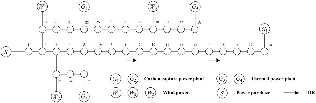
FIGURE 1. The revised IEEE-33 bus distribution system.

TABLE 1

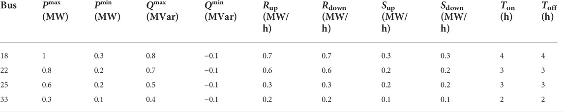
TABLE 1. The operation parameters of power plants.

TABLE 2

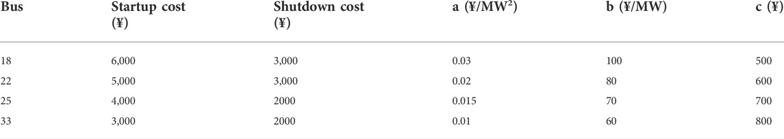
TABLE 2. The cost parameters of power plants.

TABLE 3

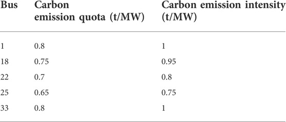
TABLE 3. The carbon emission factors of carbon emission sources.

Result analysis

Robustness and economy analysis

Due to the low probability of the extreme wind power output, the robustness and economy of the model can be balanced by adjusting the budget Γ_wind to avoid the too conservative optimization results. In this case, the budgets Γ_wind are set to 0, 2, 4 and 8, respectively. The results of outputs of power plants are shown in Figure 2. The outputs of power plants are indicated by the height of the colored bar. The initial load curve, the load curve after PDR and the load curve after PDR and IDR are presented by different curves in Figure 3. The hourly electricity prices are represented by stems in Figure 4. Figure 5 shows the sum of the forecast value, the output range and the actual output of all wind power. Table 4 shows various costs and the carbon emissions of the distribution system.

FIGURE 2

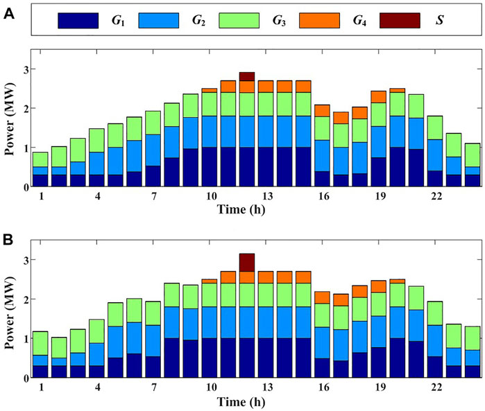
FIGURE 2. Outputs of power plants: (A) Γ_wind = 0 (B) Γ_wind = 8.

FIGURE 3

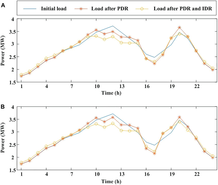
FIGURE 3. Load curves: (A) Γ_wind = 0 (B) Γ_wind = 8.

FIGURE 4

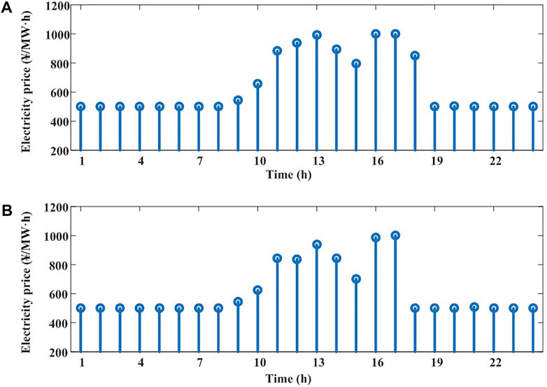
FIGURE 4. Electricity prices: (A) Γ_wind = 0 (B) Γ_wind = 8.

FIGURE 5

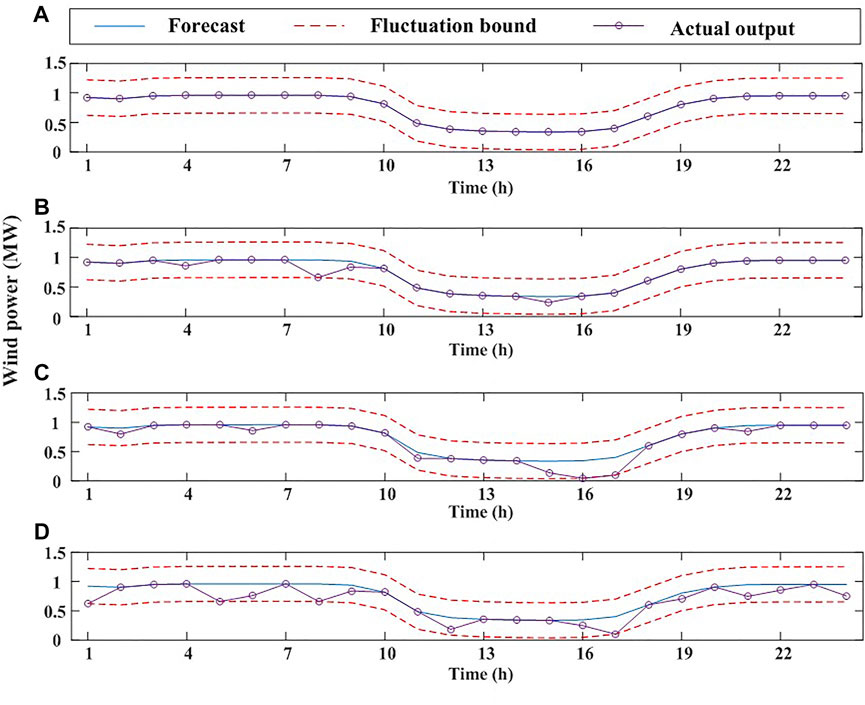
FIGURE 5. Wind power curves: (A) Γ_wind = 0 (B) Γ_wind = 2 (C) Γ_wind = 4 (D) Γ_wind = 8.

TABLE 4

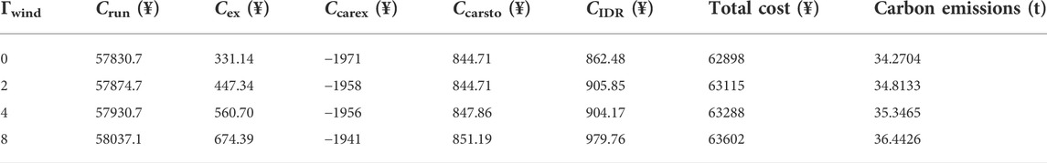
TABLE 4. Robust optimization results under different budget Γ_wind.

In Figure 2, it can be seen the outputs of power plants increase due to the uncertainty of the wind power. Especially, when all power plants reach their maximum power, the purchasing power increases significantly. At this time, power plants have no additional regulation capacity to cope with the uncertainty of the wind power. Therefore, the power balance can only be achieved by purchasing power from the main network. It can be found from Figure 3 that the peak-valley difference of the load curves decreases after the implementation of PDR and IDR. The interruptible loads are interrupted at the peak and the shiftable loads are transferred from the peak to the valley of the loads. The electricity prices are higher at the peak of the loads and lower at the valley of the loads in Figure 4. Because a smoother load curve can avoid the frequent startup and shutdown of the power plants, which can reduce the total cost. In Figure 4B, the electricity prices fluctuate between 10:00 and 13:00 instead of monotone increasing in Figure 4A. And the variations of electricity prices from 15:00 to 18:00 are larger. It is reasonable because the uncertainty of the wind power leads to the changes of power plants outputs. In order to minimize the total cost while meeting the load demand, the electricity prices will also change more. Therefore, fluctuating wind power output will lead to significant changes in electricity prices.

According to the uncertainty set, the forecast value of wind power is in the middle of the upper bound and lower bound. When the budget Γ_wind is set to 0, this model is transformed into a deterministic optimization. The actual output of wind power is consistent with the forecast value. When the budgets Γ_wind are set to 2, 4 and 8, the actual output of wind power tends to locate at the lower bound and reaches the lower bound at some time in Figure 5, which is regarded as the worst-case output of wind power. In Table 4, the various costs have increased with the increase of budget Γ_wind. Because the output of wind power is decreased. In order to meet the load demand, all costs are increased. Although the amount of carbon dioxide captured by carbon capture power plants increases, the carbon emissions of the distribution system increase from 34.2704 t to 36.4426 t.

Effect of carbon trading price

The carbon trading mechanism not only imposes economic punishment on high carbon emission power plants, but also rewards energy-saving and environmentally friendly power plants, which makes carbon emissions of great economic value. The change of carbon trading price affects various costs. The relation with the operation cost and power purchase cost is shown in Figure 6. Figure 7 shows the relation with the total cost and the carbon trading cost. When the carbon trading cost is positive, it means the profit generated by the power plants selling carbon emission quotas. When the carbon trading cost is negative, it means the cost generated by the power plant purchasing additional carbon emission quotas. The change of carbon trading price also affects the carbon emissions and the amount of captured carbon dioxide, as shown in Figure 8.

FIGURE 6

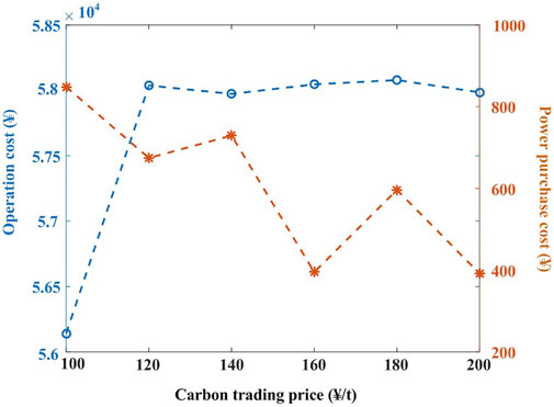
FIGURE 6. Relation curve between operation cost, power purchase cost and carbon trading price.

FIGURE 7

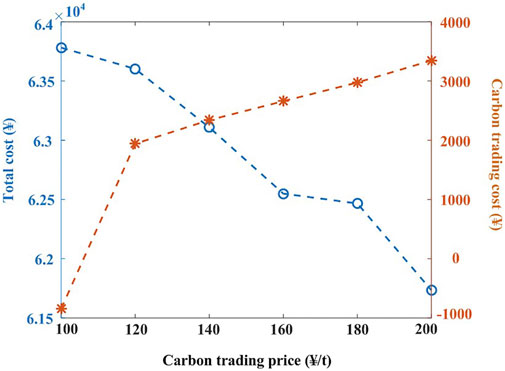
FIGURE 7. Relation curve between total cost, carbon trading cost and carbon trading price.

FIGURE 8

FIGURE 8. Relation curve between carbon emissions, carbon capture and carbon trading price.

In Figure 6, the operation cost increase at the beginning and then remain stable. When the carbon trading price is 100 ¥/t, the profit generated by carbon capture are low. Therefore, the carbon capture devices operate at a very low power and generate little cost. When the carbon trading price is 120 ¥/t or more, the profit can reduce the total cost greatly. So, carbon capture devices operate at a high power leading to the increase of operation cost. And the operation cost keeps stable when the carbon capture devices operate at the maximum power. The power purchasing cost shows a decreased trend. It is reasonable because the high carbon trading prices encourage the low-carbon power plants. The power purchase from the main network can be regarded as a high pollution thermal power plant. And the purchasing power decreases with the increase of carbon trading price.

It can be observed that the profit generated by the carbon trading increases and the total cost decreases with the increase of the carbon trading price in Figure 7. The carbon capture power plants sell carbon emission quotas to gain profit. The higher carbon trading price, the more profit. And the total cost become less.

It can be found in Figure 8 that the carbon emissions decrease at first and keep stable later. The amount of carbon dioxide captured shows a similar trend with the operation cost when the carbon trading price increase. Because the operation of carbon capture devices is the main factor that affects the operation cost. When the carbon capture devices operate at maximum power, the carbon emissions remain unchanged basically. But the basic carbon emissions are inevitable to meet the load demand.

Therefore, the carbon trading mechanism can promote energy conservation and emission reduction of power plants. Combining the carbon trading mechanism and the CCS technology will release their carbon emission reduction potential and decrease the carbon emissions of the distribution system.

Comparison of demand response

PDR and IDR dispatch loads in different ways. PDR enable user to spontaneously change their consumption habits by setting electricity prices, so the scheduling cost is 0 ¥. And IDR dispatches loads by economic compensation. In order to compare the effects of PDR and IDR, four cases are designed.

Case 1:. Demand response doesn’t participate in distribution system dispatch.

Case 2:. PDR participates in distribution system dispatch.

Case 3:. IDR participates in distribution system dispatch.

Case 4:. Both PDR and IDR participate in distribution system dispatch.Optimization results of various costs and carbon emissions are shown in Table 5. The total costs of case 1 and case 2 are basically the same, but the carbon emissions are reduced. It can be seen that PDR can decrease the carbon emissions of distribution system but has little impact on the total cost. Compared case 1 with case 3, the total cost and carbon emissions are reduced significantly. Although there is IDR scheduling cost, IDR has a significant effect on reducing total cost and carbon emissions compared with PDR. When both PDR and IDR participate in distribution system dispatch at the same time, the power purchase cost is reduced greatly so that the total cost are decreased to the minimum in case 4. Because of the participation of demand response, the loads are more easily met by the power plants of the distribution network with no need to purchase power from the main network. And the carbon emissions are the lowest among four cases. Therefore, the participation of PDR and IDR in distribution system can realize the optimization of economic and environmental benefits.

TABLE 5

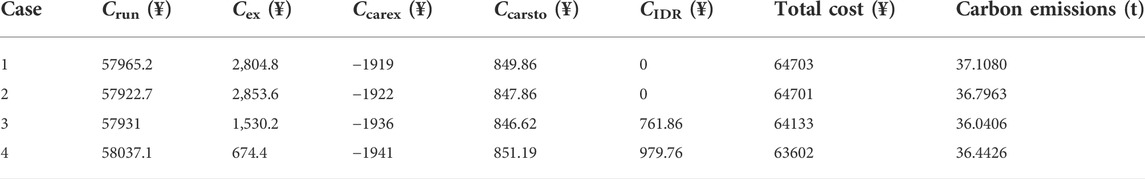
TABLE 5. Robust optimization results under different cases.

Conclusion

In this paper, a two-stage robust optimal dispatch model of the distribution system considering carbon capture and demand response is proposed. This model takes the uncertainty of wind power into account and realize the low-carbon economic operation of the distribution system. From the results of case studies, the following conclusions can be drawn: 1) With the increasing uncertainty of the wind power, all costs and carbon emissions of the distribution system increase. The robustness and economy of the model can be balanced by adjusting the budget Γ_wind to avoid the too conservative optimization results. 2) PDR and IDR can reduce the peak-valley difference of the load curves to realize the optimization of economic and environmental benefits. And the uncertainty of wind power can lead to the fluctuation of electricity prices. 3) The carbon trading mechanism can promote energy conservation and emission reduction of power plants. Carbon capture devices can capture carbon dioxide more by setting carbon trading price reasonably. However, the actual operation process of the carbon capture power plant is complex. Further work will consider a more detailed model of the carbon capture power plant. And a more accurate representation of wind power uncertainty is worthy of study.

Data availability statement

The original contributions presented in the study are included in the article/Supplementary Material, further inquiries can be directed to the corresponding author.

Author contributions

YG contributed to the model, simulation and writing. CW contributed to the method. YH and GH contributed equally to the editing of the article and discussion. YL contributed to the literature analysis and provided a critical review.

Funding

This work was supported by the National Natural Science Foundation of China (52277088 and 51907050).

Conflict of interest

YH was employed by the Company State Grid Jiangsu Electric Power Co., Ltd.

The remaining authors declare that the research was conducted in the absence of any commercial or financial relationships that could be construed as a potential conflict of interest.

Publisher’s note

All claims expressed in this article are solely those of the authors and do not necessarily represent those of their affiliated organizations, or those of the publisher, the editors and the reviewers. Any product that may be evaluated in this article, or claim that may be made by its manufacturer, is not guaranteed or endorsed by the publisher.

References

Akbari-Dibavar, A., Mohammadi-Ivatloo, B., Zare, K., Khalili, T., and Bidram, A. (2021). Economic-emission dispatch problem in power systems with carbon capture power plants. IEEE Trans. Ind. Appl. 57, 3341–3351. doi:10.1109/TIA.2021.3079329

CrossRef Full Text | Google Scholar

Bai, L., Li, F., Cui, H., Jiang, T., Sun, H., and Zhu, J. (2016). Interval optimization based operating strategy for gas-electricity integrated energy systems considering demand response and wind uncertainty. Appl. Energy 167, 270–279. doi:10.1016/j.apenergy.2015.10.119

CrossRef Full Text | Google Scholar

Chen, Q., Kang, C., Xia, Q., and Kirschen, D. S. (2012). Optimal flexible operation of a CO₂ capture power plant in a combined energy and carbon emission market. IEEE Trans. Power Syst. 27, 1602–1609. doi:10.1109/TPWRS.2012.2185856

CrossRef Full Text | Google Scholar

Chen, Q., Kang, C., and Xia, Q. (2010). Modeling flexible operation mechanism of CO₂ capture power plant and its effects on power-system operation. IEEE Trans. Energy Convers. 25, 853–861. doi:10.1109/TEC.2010.2051948

CrossRef Full Text | Google Scholar

Chen, X., Huang, L., Zhang, X., He, S., Sheng, Z., Wang, Z., et al. (2021). Robust optimal dispatching of wind fire energy storage system based on equilibrium optimization algorithm. Front. Energy Res. 9, 754908. doi:10.3389/fenrg.2021.754908

CrossRef Full Text | Google Scholar

Dolatabadi, S. H., Ghorbanian, M., Siano, P., and Hatziargyriou, N. D. (2021). An enhanced IEEE 33 bus benchmark test system for distribution system studies. IEEE Trans. Power Syst. 36, 2565–2572. doi:10.1109/TPWRS.2020.3038030

CrossRef Full Text | Google Scholar

Ji, Z., Kang, C., Chen, Q., Xia, Q., Jiang, C., Chen, Z., et al. (2013). Low-carbon power system dispatch incorporating carbon capture power plants. IEEE Trans. Power Syst. 28, 4615–4623. doi:10.1109/TPWRS.2013.2274176

CrossRef Full Text | Google Scholar

Kirschen, D. S., Strbac, G., Cumperayot, P., and de Paiva Mendes, D. (2000). Factoring the elasticity of demand in electricity prices. IEEE Trans. Power Syst. 15, 612–617. doi:10.1109/59.867149

CrossRef Full Text | Google Scholar

Lei, H., Huang, S., Liu, Y., and Zhang, T. (2019). Robust optimization for microgrid defense resource planning and allocation against multi-period attacks. IEEE Trans. Smart Grid 10, 5841–5850. doi:10.1109/TSG.2019.2892201

CrossRef Full Text | Google Scholar

Lei, S., Hou, Y., Qiu, F., and Yan, J. (2018). Identification of critical switches for integrating renewable distributed generation by dynamic network reconfiguration. IEEE Trans. Sustain. Energy 9, 420–432. doi:10.1109/TSTE.2017.2738014

CrossRef Full Text | Google Scholar

Li, J., Wen, J., and Han, X. (2015). Low-carbon unit commitment with intensive wind power generation and carbon capture power plant. J. Mod. Power Syst. Clean. Energy 3, 63–71. doi:10.1007/s40565-014-0095-6

CrossRef Full Text | Google Scholar

Liu, G., and Tomsovic, K. (2015). Robust unit commitment considering uncertain demand response. Electr. Power Syst. Res. 119, 126–137. doi:10.1016/j.epsr.2014.09.006

CrossRef Full Text | Google Scholar

Liu, Y., Guo, L., and Wang, C. (2018). A robust operation-based scheduling optimization for smart distribution networks with multi-microgrids. Appl. Energy 228, 130–140. doi:10.1016/j.apenergy.2018.04.087

CrossRef Full Text | Google Scholar

Lou, S., Lu, S., Wu, Y., and Kirschen, D. S. (2015). Optimizing spinning reserve requirement of power system with carbon capture plants. IEEE Trans. Power Syst. 30, 1056–1063. doi:10.1109/TPWRS.2014.2341691

CrossRef Full Text | Google Scholar

Reddy, K. S., Panwar, L. K., Panigrahi, B. K., and Kumar, R. (2017). Modeling of carbon capture technology attributes for unit commitment in emission-constrained environment. IEEE Trans. Power Syst. 32, 662–671. doi:10.1109/TPWRS.2016.2558679

CrossRef Full Text | Google Scholar

Wang, C., Ju, P., Wu, F., Lei, S., and Pan, X. (2022). Long-term voltage stability-constrained coordinated scheduling for gas and power Grids with uncertain wind power. IEEE Trans. Sustain. Energy 13, 363–377. doi:10.1109/TSTE.2021.3112983

CrossRef Full Text | Google Scholar

Wang, C., Lei, S., Ju, P., Chen, C., Peng, C., and Hou, Y. (2020b). MDP-Based distribution network reconfiguration with renewable distributed generation: Approximate dynamic programming approach. IEEE Trans. Smart Grid 11, 3620–3631. doi:10.1109/TSG.2019.2963696

CrossRef Full Text | Google Scholar

Wang, J., Xu, Q., Su, H., and Fang, K. (2021). A distributed and robust optimal scheduling model for an active distribution network with load aggregators. Front. Energy Res. 9, 646869. doi:10.3389/fenrg.2021.646869

CrossRef Full Text | Google Scholar

Wang, X., Shahidehpour, M., Jiang, C., and Li, Z. (2019). Coordinated planning strategy for electric vehicle charging stations and coupled traffic-electric networks. IEEE Trans. Power Syst. 34, 268–279. doi:10.1109/TPWRS.2018.2867176

CrossRef Full Text | Google Scholar

Wang, Y., Qiu, J., Tao, Y., and Zhao, J. (2020a). Carbon-oriented operational planning in coupled electricity and emission trading markets. IEEE Trans. Power Syst. 35, 3145–3157. doi:10.1109/TPWRS.2020.2966663

CrossRef Full Text | Google Scholar

Xiao, H., Pei, W., Dong, Z., and Kong, L. (2018). Bi-level planning for integrated energy systems incorporating demand response and energy storage under uncertain environments using novel metamodel. CSEE J. Power Energy Sys 4, 155–167. doi:10.17775/CSEEJPES.2017.01260

CrossRef Full Text | Google Scholar

Xu, L., Guo, Q., Yang, T., and Sun, H. (2019). Robust routing optimization for smart grids considering cyber-physical interdependence. IEEE Trans. Smart Grid 10, 5620–5629. doi:10.1109/TSG.2018.2888629

CrossRef Full Text | Google Scholar

Yan, D., Wang, S., Zhao, H., Zuo, L., Yang, D., Wang, S., et al. (2022). A robust scheduling methodology for integrated electric-gas system considering dynamics of natural gas pipeline and blending hydrogen. Front. Energy Res. 10, 863374. doi:10.3389/fenrg.2022.863374

CrossRef Full Text | Google Scholar

Zeng, B., and Zhao, L. (2013). Solving two-stage robust optimization problems using a column-and-constraint generation method. Operations Res. Lett. 41, 457–461. doi:10.1016/j.orl.2013.05.003

CrossRef Full Text | Google Scholar

Zhang, B., Li, Q., Wang, L., and Feng, W. (2018). Robust optimization for energy transactions in multi-microgrids under uncertainty. Appl. Energy 217, 346–360. doi:10.1016/j.apenergy.2018.02.121

CrossRef Full Text | Google Scholar

Zhang, N., Hu, Z., Dai, D., Dang, S., Yao, M., and Zhou, Y. (2016a). Unit commitment model in smart grid environment considering carbon emissions trading. IEEE Trans. Smart Grid 7, 420–427. doi:10.1109/TSG.2015.2401337

CrossRef Full Text | Google Scholar

Zhang, X., Shahidehpour, M., Alabdulwahab, A., and Abusorrah, A. (2016b). Hourly electricity demand response in the stochastic day-ahead scheduling of coordinated electricity and natural gas networks. IEEE Trans. Power Syst. 31, 592–601. doi:10.1109/TPWRS.2015.2390632

CrossRef Full Text | Google Scholar

Zhao, C., Wang, J., Watson, J., and Guan, Y. (2013). Multi-stage robust unit commitment considering wind and demand response uncertainties. IEEE Trans. Power Syst. 28, 2708–2717. doi:10.1109/TPWRS.2013.2244231

CrossRef Full Text | Google Scholar

Zhou, Y., Yu, H., Li, Z., Su, J., and Liu, C. (2020). Robust optimization of a distribution network location-routing problem under carbon trading policies. IEEE Access 8, 46288–46306. doi:10.1109/ACCESS.2020.2979259

CrossRef Full Text | Google Scholar

Zhu, X., Wu, J., and Liu, D. (2022). Robust unit commitment for minimizing wind spillage and load shedding with optimal DPFC. Front. Energy Res. 10, 877042. doi:10.3389/fenrg.2022.877042

CrossRef Full Text | Google Scholar