Extended state observer-based predictive control for soft open point

1 Introduction

In recent years, many benefits have been brought by the application of increasing renewable energy sources. However, many problems may occur when renewable energy sources are connected to the distribution network, such as power imbalance and voltage instability (Rueda and Padilha, 2013; Gong et al., 2021). As a power electronic device, Soft Open Point (SOP) has many advantages, such as connecting lines at different voltage levels, flexibly regulating the power flow in the system, fast system response, and diverse control methods. Therefore, SOP is widely used in distribution networks (Jiang et al., 2022). Two-port SOP can be considered as a back-to-back voltage source converter (VSC) consisting of a rectifier-side VSC, an inverter-side VSC, and a DC capacitor (Wu et al., 2018). The mathematical model of SOP is a non-linear system with solid coupling characteristics, including the uncertainty of external disturbances and parameter perturbations, which significantly complicates the controller design (Huo et al., 2021; Liang et al., 2022). Some traditional control methods of SOP are widely used in SOP systems, including proportional-integral (PI) control, model predictive control (MPC), and droop control (Cao et al., 2016; Cai et al., 2018; Falkowski and Sikorski, 2018; Li et al., 2020; Zhang et al., 2021). However, the traditional PI control has many parameters, bringing parameter design problems. The robustness of PI control and droop control is poor when disturbances are occurred in SOP systems (Li et al., 2019). In Figure 1, the system structure of the two-port SOP is shown.

FIGURE 1

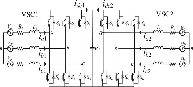
FIGURE 1. Model of two-port SOP.

Compared with traditional control methods, the MPC method is widely used in the design of power electronic converters due to its simple structure, easy implementation, and sound control effect (Zhang et al., 2017a). The basic principle of MPC is to use the mathematical model of the controlled object, discretize it to get the predicted value of the next moment, and then optimize the cost function to make the predicted value along the reference trajectory and converge to the desired value. However, the MPC method relies on the mathematical model of the controlled object, which is subject to internal parameter drift and unknown external disturbances during system operation. This will result in a degradation of control performance and a reduction of control accuracy (Young et al., 2016; Zhang et al., 2019). In order to make the system more robust and dynamic, the inter-loop and outer-loop of the control system need to be redesigned (Zhang et al., 2017b; Liu et al., 2018).

In order to solve the above problems, various improved methods are proposed for the inner-loop. In (Pamshetti et al., 2021), a single-vector-based model predictive controller is proposed to control the inner-loop, which has the disadvantage of leading to significant current harmonics and power fluctuations. In (Wang et al., 2021a), an improved MPC method based on three-vector (TV-MPC) is proposed to reduce the current harmonics and power fluctuations effectively, which has better dynamic performance and robustness of the system. In (Liu and Gao, 2020), an improved model predictive direct control method is proposed to calculate the desired voltage vector through the deadbeat control theory. The virtual voltage vector introduced is used to determine the sector where the desired voltage is located, and then the actual voltage is calculated. The results show that the method can effectively improve the robustness. In (Morsi et al., 2021), a linear variable parameter MPC method is proposed. A new predictive model and a new cost function are built by designing incremental forms to overcome the steady-state errors caused by model parameter mutations and external disturbances. And the experimental results show that the method has good dynamic stability.

In (Morsi and Cedric, 2021), in order to reduce the influence of the parameter perturbation of the control model, a model-free control method is proposed, which only considers the input and output of the outer-loop, and any other parameters are not involved. The known and unknown term disturbances are referred to as the total disturbances in the system. Thus, the influence of system parameters and external disturbances on the control performance is avoided, the dependence of the model on parameters is reduced, and the control performance is improved. In (Wang and Li, 2021), an ultra-local model-free and deadbeat predictive control method are proposed for permanent magnet synchronous motor (PMSM). An ultra-local control model is established using the input and output variables of the outer-loop. The results show that the method can effectively improve the robustness of the model and has a strong anti-interference ability. In (Zhou et al., 2016), an ultra-local model-free control model is established to solve the problem of total system disturbance term in PMSM. Moreover, the results show that the method reduces the current harmonics and improves the system’s dynamic response performance.

In this paper, by introducing the ultra-local model-free control algorithm and TV-MPC theory, an ESO-based ultra-local model-free voltage prediction method and a current TV-MPC method are proposed. Using the input and output of the voltage outer-loop, ESO is established to observe the total disturbance of the system and compensate for the one-beat delay of the control system in real-time. The frequency domain analysis method is also used to adjust the ESO parameters so that the system can deal with external disturbances, which have better robustness and dynamic performance. The contributions of this article are listed as follows.

1) Compared with the traditional single-vector MPC method of the inner-loop, in this article, the TV-MPC method is used in the inner-loop of the SOP system, which improves the current harmonics effectively.

2) Compared with the traditional PI method of the outer-loop, in this article, an ultra-local model-free voltage prediction method is used in the outer-loop, which improves the anti-interference and robustness of the SOP control system.

3) ESO is established to observe the total disturbance and compensate for the delay of the system in real time, which improves the robustness of the SOP system.

The organization of this article is as follows: Section 2 introduces the model of the two-port SOP system. In Section 3, the sensitivity of the system parameters is analyzed. In Section 4, the ESO-based ultra-local model-free voltage outer-loop prediction controller is designed. In Section 5, the TV-MPC method for SOP systems is proposed. Section 6 gives the simulation results. Section 7 discusses the future work that needs to be improved and summarizes the conclusions.

2 Mathematical models of Soft Open Point

In Figure 1, it can be seen that the two-port SOP has symmetry in structure, so one of the voltage inverters (VSC1) is selected to form the port1, which has the specific structure as shown in Figure 2 (Wang et al., 2021b).

FIGURE 2

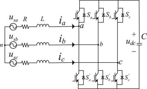
FIGURE 2. Model of VSC1.

Where C is the DC-side filter capacitor; R is the AC-side equivalent connection resistance; L is the AC-side equivalent connection inductor. Assume that the three-phase voltage at each port is balanced, and from the direction of current in Figure 1, the port1 model can be expressed as:

$L\frac{\mathrm{d}{i}_m}{\mathrm{d}t}=u_{sm}-R{i}_m-S_m{u}_{dc}+\frac{1}{3}{u}_{dc}\left(S_a+S_b+S_c\right)(1)$

Where S_m is the modulation switch function of VSC1; m represents abc three-phases; u_dc is the DC-side voltage; u_sm is the AC-side voltage; i_m is the AC-side current. The other ports in the SOP have the same strongly coupled mathematical model.

Eq. 1 is transformed by Park. The equivalent equation of the d- and q-axis components are obtained (Hur et al., 2001):

$\left\{\begin{array}{l}L\frac{\mathrm{d}{i}_d}{\mathrm{d}t}=-R{i}_d+{\omega }_{1}L{i}_q+u_d-S_d{u}_{dc}\\ L\frac{\mathrm{d}{i}_q}{\mathrm{d}t}=-R{i}_q-{\omega }_{1}L{i}_d+u_q-S_q{u}_{dc}\end{array}\right.(2)$

Where i_d and i_q are the d- and q-axis currents of VSC1, respectively. u_d and u_q are the d- and q-axis grid voltages of VSC1. ω₁ is the phase voltage angular frequency of the AC-side of VSC1. S_d and S_q are the components of the modulation switch function of VSC1 in the d- and q-axis. Similarly, VSC2 has the same mathematical model in the synchronous rotating frame.

According to the current direction shown in Figure 1, the DC-side current can be expressed as follows:

$\left\{\begin{array}{l}{i}_{dc}=C\frac{\mathrm{d}{u}_{dc}}{\mathrm{d}t}={\displaystyle \sum _{k=\mathrm{1,2}}}{i}_{dc,k}=i_{dc,1}+i_{dc,2}\\ i_{dc,k}={\displaystyle \sum _{i=a,b,c}}{S}_{ik}{i}_{ik}=S_{ak}{i}_{ak}+S_{bk}{i}_{bk}+S_{ck}{i}_{ck}\end{array}\right.(3)$

Where i_dc,k is the DC-side current of Port k; S_ik is the modulation switch function of the abc three-phases of Port k; i_ik is the output current of the abc three phases of Port k. Taking Eq. 3 and passing it through the Park transformation, the equivalent equation of the d-axis and q-axis components is obtained:

$i_{dc}=C\frac{\mathrm{d}{u}_{dc}}{\mathrm{d}t}=\frac{3}{2}{\displaystyle \sum _{k=\mathrm{1,2}}}\left(-S_{dk}{i}_{dk}+S_{qk}{i}_{qk}\right)(4)$

Where S_dk and S_qk are the modulation switch function of the d- and q-axis of Port k; i_dc is the DC-side current; i_dk and i_qk are the d- and q-axis currents of the Port k; u_dk and u_qk are the d- and q-axis voltages of the Port k, respectively.

According to the instantaneous reactive power theory, the active power and reactive power output from each port can be expressed on the d- and q-axis as follows (Zhang et al., 2018):

$\left\{\begin{array}{l}{P}_k=\frac{3}{2}\left(i_{dk}{u}_{dk}+i_{qk}{u}_{qk}\right)\\ Q_k=\frac{3}{2}\left(i_{dk}{u}_{qk}-i_{qk}{u}_{dk}\right)\end{array}\right.k=\mathrm{1,2}(5)$

The system three-phase voltage is balanced. If the direction of the d-axis coincides with the direction of the AC system voltage vector u_s, the state of the d- and q-axis currents of AC-side i_dk and i_qk can be written as:

$\left\{\begin{array}{l}{i}_{dk}=C\\ i_{qk}=0\end{array}\right.(6)$

Substituting (6) into (5), the active and reactive power of the Port k can be written as:

$\left\{\begin{array}{l}{P}_k=\frac{3}{2}{i}_{dk}{u}_{dk}\\ Q_k=-\frac{3}{2}{i}_{qk}{u}_{dk}\end{array}\right.k=\mathrm{1,2}(7)$

From (7), it can be seen that the active and reactive power on the AC-side of each port is proportional to the amount of current in the d- and q-axis, respectively. Moreover, the decoupling control of independence of active and reactive power can be realized by controlling the amount of current in the d- and q-axis (Zhang et al., 2020). After the coordinate transformation, the established system model is simplified, and the controller design of the system is convenient.

According to different distribution network operating requirements, the SOP can operate in three different operating modes: U_dcQ mode, PQ mode and V/f mode. Among them, one port must work in U_dcQ mode when the system is in regular operation to maintain voltage stability on the DC-side. PQ mode is most used in the working operation state, which can regulate the active and reactive power of the system individually. The V/f mode operates where a port needs to be switched to a fixed AC-voltage mode to supply power to the fault area load. In this paper, port1 uses U_dcQ mode, and port2 uses PQ mode (Wang et al., 2022).

3 Parameter sensitivity analysis

From (4), it is clear that:

$i_{dc}=C\frac{\mathrm{d}{u}_{dc}}{\mathrm{d}t}=\frac{3}{2}\left(-S_{d1}{i}_{d1}-S_{d2}{i}_{d2}\right)(8)$

According to Eq. 8, the voltage equation can be written as follows:

$\frac{\mathrm{d}{u}_{dc}}{\mathrm{d}t}=\frac{3}{2C}\left(S_{d1}{i}_{d1}+S_{d2}{i}_{d2}\right)(9)$

By discretizing Eq. 2 and Eq. 9, the equation can be written as follows:

$\left\{\begin{array}{l}{u}_{dc}\left(k+1\right)=u_{dc}\left(k\right)+\frac{3T_s}{2C}\left(-S_{d1}{i}_{d1}-S_{d2}{i}_{d2}\right)\\ i_{d1}\left(k+1\right)=\left(1-\frac{R_1{T}_s}{L_1}\right)i_{d1}\left(k\right)+T_s{\omega }_1{i}_{q1}\left(k\right)+\frac{T_s}{L_1}\left(u_{d1}\left(k\right)-u_{1dN}\left(k\right)\right)\\ i_{d2}\left(k+1\right)=\left(1-\frac{R_2{T}_s}{L_2}\right)i_{d2}\left(k\right)+T_s{\omega }_2{i}_{q2}\left(k\right)+\frac{T_s}{L_2}\left(u_{d2}\left(k\right)-u_{2dN}\left(k\right)\right)\end{array}\right.(10)$

Where k+1 means the value of the variable at the next moment and k means the value of the variable at the current moment; T_s is the sampling time; u_1dN and u_2dN are the d-axis voltages of VSC1 and VSC2, respectively; ω₁ and ω₂ are the phase voltage angular frequency of the AC-side of VSC1 and VSC2. Conventional controllers need to consider L, C and other parameters, and the control accuracy is more dependent on the accuracy of the control parameters. To analyze the impact of parameter ingestion on the controller, assuming that R₀, L₀ and C₀ are the actual resistor, inductor and capacitor, then Eq. 10 can be rewritten as follows:

$\left\{\begin{array}{l}{\widehat{u}}_{dc}\left(k+1\right)=u_{dc}\left(k\right)+\frac{3T_s}{2C_0}\left(-S_{d1}{\widehat{i}}_{d1}-S_{d2}{\widehat{i}}_{d2}\right)\\ {\widehat{i}}_{d1}\left(k+1\right)=\left(1-\frac{R_{10}{T}_s}{L_{10}}\right)i_{d1}\left(k\right)+T_s{\omega }_1{i}_{q1}\left(k\right)+\frac{T_s}{L_{10}}\left(u_{d1}\left(k\right)-u_{1Nd}\left(k\right)\right)\\ {\widehat{i}}_{d2}\left(k+1\right)=\left(1-\frac{R_{20}{T}_s}{L_{20}}\right)i_{d2}\left(k\right)+T_s{\omega }_2{i}_{q2}\left(k\right)+\frac{T_s}{L_{20}}\left(u_{d2}\left(k\right)-u_{2Nd}\left(k\right)\right)\end{array}\right.(11)$

In (11), ${\widehat{i}}_{d1}$, ${\widehat{i}}_{d2}$ and ${\widehat{u}}_{dc}$ are the estimated value of the variables of i_d1, i_d2 and u_dc at the time of parametric perturbation, and the voltage error can be written as follows:

$\left\{\begin{array}{c}\Delta \mathrm{\Psi }={\widehat{u}}_{dc}\left(k+1\right)-u_{dc}\left(k+1\right)=\Delta {\mathrm{\Psi }}_1+\Delta {\mathrm{\Psi }}_2\\ \Delta {\mathrm{\Psi }}_1=\frac{3T_s{S}_{d1}}{2}\left(\frac{1}{C}-\frac{1}{C_0}\right)\left(i_{d1}+T_s{\omega }_1{i}_{q1}\right)+\frac{3T_s^2{i}_{d1}}{2}\left(\frac{R_{10}}{C_0{L}_{10}}-\frac{R_1}{C{L}_1}\right)\\ +\frac{3T_s{S}_{d1}}{2}\left(\frac{1}{C{L}_1}-\frac{1}{C_0{L}_{10}}\right)T_s\left(u_{d1}\left(k\right)-u_{1Nd}\left(k\right)\right)\\ \Delta {\mathrm{\Psi }}_2=\frac{3T_s{S}_{d2}}{2}\left(\frac{1}{C}-\frac{1}{C_0}\right)\left(i_{d2}+T_s{\omega }_2{i}_{q2}\right)+\frac{3T_s^2{i}_{d2}}{2}\left(\frac{R_{20}}{C_0{L}_{20}}-\frac{R_2}{C{L}_2}\right)\\ +\frac{3T_s{S}_{d2}}{2}\left(\frac{1}{C{L}_2}-\frac{1}{C_0{L}_{20}}\right)T_s\left(u_{d2}\left(k\right)-u_{2Nd}\left(k\right)\right)\end{array}\right.(12)$

Where $\Delta {\mathrm{\Psi }}_1$ and $\Delta {\mathrm{\Psi }}_2$ are the voltage errors generated by VSC1 and VSC2. From (12), it can be seen that the L and the DC-side C significantly impact the prediction error in the system. In order to reduce the dependence on the system model and improve the robustness of the system, this article proposes an ultra-local model-free predictive control method based on the ESO.

4 Design of expansion state observer -based ultra-local model-free voltage prediction control

4.1 Traditional voltage loop control strategy

Traditional PI voltage control is based on error elimination control, which can lead to excessive overshoot and oscillation of the system if the initial value is too large. Moreover, the traditional control method has an inevitable delay for system model parameter perturbations and disturbances.

This article proposes an ultra-local model-free predictive control method based on the ESO, which uses only the inputs and outputs of the system without considering any parameters, and views known and unknown perturbations as total perturbations. The external perturbations observed by the ESO are also used to implement feedback compensation to reduce model dependence on parameters and improve system robustness.

4.2 Ultra-local model

For the input and output of the system, the traditional ultra-local model can be written as follows (Morsi and Cedric, 2021):

$\dot{y}=\alpha u+F(13)$

Where y is the output of the system; u is the input of the system; F is regarded as the total disturbance of the system; α is the model self-attribute parameter. The controller can be designed as follows:

$\left\{\begin{array}{l}u=\frac{{\dot{y}}_{\exp }-\widehat{F}+\zeta }{\alpha }\\ \dot{e}+\zeta =0\end{array}\right.(14)$

Where y_exp is the expected output of the system; $e=y_{\exp }-y$, that e is the tracking error; $\widehat{F}$ is an estimate of the total disturbance; and ζ is the designed controller output.

4.3 Design of ultra-local model-free outer-loop prediction controller

Taking i_d1 in (9) as the output of the outer-loop system and u_dc as the input of the outer-loop system, the ultra-local model-free control structure is established as follows:

$\frac{\mathrm{d}{u}_{dc}}{\mathrm{d}t}=k_1{i}_{d1}+F(15)$

Where k₁ is the controller gain. Using the forward Eulerian discretization method, Eq. 15 is discretized to transform the continuous time model into the discrete time model. And the ultra-local model-free control structure can be rewritten as:

$u_{dc}\left(k+1\right)=u_{dc}\left(k\right)+T_s\left[k_1{i}_{d1}\left(k\right)+\widehat{F}\left(k\right)\right](16)$

The output of the controller can be written as follows:

$i_{d1}\left(k\right)=\frac{u_{dc}\left(k+1\right)-u_{dc}\left(k\right)-T_s\widehat{F}\left(k\right)}{k_1{T}_s}(17)$

To have better tracking of the rated voltage, let u_dc (k + 1) = u_dcref, thus Eq. 17 can be rewritten as:

$i_{d1ref}\left(k\right)=\frac{u_{dcref}-u_{dc}\left(k\right)-T_s\widehat{F}\left(k\right)}{k_1{T}_s}(18)$

In order to improve the system control performance and solve the system time delay problem, the ESO is designed to compensate for the time delay effect.

4.4 Design of expansion state observer

According to Eq. 15, the outer-loop input i_d1 and the system total disturbance F are chosen as state variables to design the ESO, and the state space equation is obtained as follows (Chi et al., 2020; Yang et al., 2020):

$\left\{\begin{array}{l}{\dot{z}}_1=z_1+k_1{i}_{d1}-{\alpha }_{1}e\\ {\dot{z}}_2=-{\alpha }_{2}e\\ e=z_1-u_{dc}\end{array}\right.(19)$

Where α₁ and α₂ are the observer gain coefficients; $z_1={\widehat{u}}_{dc}$, that z₁ is the estimated value of u_dc; $z_2=\widehat{F}$, that z₂ is the estimated value of F. Figure 3 shows the block diagram of the variables state.

FIGURE 3

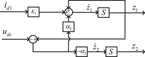
FIGURE 3. Block diagram of the variables state.

Taking Eq. 19 into Laplace transform, the transfer function of the system can be obtained:

$z_1\left(s\right)=\frac{\left({\alpha }_{1}s+{\alpha }_2\right)u_{dc}+k_1{i}_{d1}s}{s^2+{\alpha }_{1}s+{\alpha }_2}(20)$

From (20), the characteristic equation can be obtained:

$s^2+{\alpha }_{1}s+{\alpha }_2=0(21)$

In (21), it can be derived that the eigenvalue is -ω₀, where ω₀ is the bandwidth of the ESO, so the gain coefficients α₁ and α₂ of the observer are 2ω₀ and ω₀².

Using the forward Eulerian discretization method, Eq. 19 is discretized to transform the continuous time model into the discrete time model. The discrete state space equation can be written as:

$\left\{\begin{array}{l}{\widehat{u}}_{dc}\left(k+1\right)={\widehat{u}}_{dc}\left(k\right)+T_s\left[\widehat{F}\left(k\right)+k_1{i}_{d1}\left(k\right)-{\alpha }_{1}e\left(k\right)\right]\\ \widehat{F}\left(k+1\right)=\widehat{F}\left(k\right)-T_s{\alpha }_{2}e\left(k\right)\\ e\left(k\right)={\widehat{u}}_{dc}\left(k\right)-u_{dc}\left(k\right)\end{array}\right.(22)$

4.5 Stability analysis

To ensure the stability of the state of the discretized system, the characteristic roots of the characteristic equation must lie within the unit circle according to the Joly stability criterion.

By performing a Z-transformation, Eq. 22 can be rewritten as:

$\left\{\begin{array}{l}z{\widehat{u}}_{dc}\left(z\right)={\widehat{u}}_{dc}\left(z\right)+T_s\left[\widehat{F}\left(z\right)+k_1{i}_{d1}\left(z\right)-{\alpha }_{1}e\left(z\right)\right]\\ z\widehat{F}\left(z\right)=\widehat{F}\left(z\right)-T_s{\alpha }_{2}e\left(z\right)\\ e\left(z\right)={\widehat{u}}_{dc}\left(z\right)-u_{dc}\left(z\right)\end{array}\right.(23)$

Considering that the sampling time T_s is sufficiently short, the transfer function of the discrete system can be written as:

$G\left(z\right)=\frac{{\widehat{u}}_{dc}}{u_{dc}}=\frac{{\alpha }_2^{\prime }{T}_s+{\alpha }_1^{\prime }z-{\alpha }_1^{\prime }}{{\left(z-1\right)}^2+{\alpha }_2^{\prime }{T}_s+{\alpha }_1^{\prime }z-{\alpha }_1^{\prime }}(24)$

Where ${\alpha }_1^{\prime }={\alpha }_1{T}_s$; ${\alpha }_2^{\prime }={\alpha }_2{T}_s$. In (24), the characteristic equation of the system is given by:

${\left(z-1\right)}^2+{\alpha }_2^{\prime }{T}_s+{\alpha }_1^{\prime }z-{\alpha }_1^{\prime }=0(25)$

Bringing $z=\left(\lambda +1\right)/\left(\lambda -1\right)$ into Eq. 25, the characteristic equation in the λ-domain can be written as:

${\alpha }_2^{\prime }{T}_s{\lambda }^2+2\left({\alpha }_1^{\prime }-{\alpha }_2^{\prime }{T}_s\right)\lambda +\left(4+{\alpha }_2^{\prime }{T}_s-{\alpha }_1^{\prime }\right)=0(26)$

According to the Routh–Hurwitz stability criterion (Xu et al., 2020), the discrete system is stable when the following conditions are satisfied:

$\left\{\begin{array}{l}{\alpha }_2^{\prime }{T}_s<{\alpha }_1^{\prime }<{\alpha }_2^{\prime }{T}_s+4\\ {\alpha }_2^{\prime }>0\end{array}\right.(27)$

When ${\alpha }_1^{\prime }$ and ${\alpha }_2^{\prime }$ are satisfied in the equation above, the discrete system is stable. The proof is completed.

To solve the time delay problem in the system, the deadbeat principle is used. Replacing u_dc(k) and $\widehat{F}\left(k\right)$ in (18) with ${\widehat{u}}_{dc}\left(k+1\right)$ and $\widehat{F}\left(k+1\right)$ in (22), the d-axis reference currents is obtained as follows:

$i_{d1ref}\left(k\right)=\frac{u_{dcref}-{\widehat{u}}_{dc}\left(k+1\right)-T_s\widehat{F}\left(k+1\right)}{k_1{T}_s}(28)$

The current reference value is obtained by predicting the voltage value through ESO. The observed disturbances are compensated by feedback to improve the robustness of the system. Thus, the ESO-based ultra-local model-free predictive control (ULMFPC) voltage outer-loop is designed as follows:

$\left\{\begin{array}{l}{\widehat{u}}_{dc}\left(k+1\right)={\widehat{u}}_{dc}\left(k\right)+T_s\left[\widehat{F}\left(k\right)+k_1{i}_{d1}\left(k\right)-{\alpha }_{1}e\left(k\right)\right]\\ \widehat{F}\left(k+1\right)=\widehat{F}\left(k\right)-T_s{\alpha }_{2}e\left(k\right)\\ e\left(k\right)={\widehat{u}}_{dc}\left(k\right)-u_{dc}\left(k\right)\\ i_{d1ref}\left(k\right)=\frac{u_{dcref}-{\widehat{u}}_{dc}\left(k+1\right)-T_s\widehat{F}\left(k+1\right)}{k_1{T}_s}\end{array}\right.(29)$

Figure 4 shows the block diagram of outer-loop ESO-based ULMFPC.

FIGURE 4

FIGURE 4. Block diagram of outer-loop ESO-based ULMFPC.

5 Inner-loop TV- model predictive control current control for Soft Open Point

5.1 Traditional model predictive control method

Different from the current inner-loop PI control, the conventional MPC replaces the two current inner-loops of vector control with a model predictive controller, which eliminates the complex PI rectification (Li et al., 2019).

In a two-port SOP system, eight VSC voltage vectors can be selected. Six of them are non-zero vectors (V₁, V₂, V₃, V₄, V₅, V₆) and two of them are zero vectors (V₀, V₇). The eight vectors are shown in Figure 5.

FIGURE 5

FIGURE 5. Voltage vector of VSC.

The current value at the momentk is used as the basis to construct the current value at the moment k+1. The current reference value and the predicted current obtained from the prediction calculation are constituted into a cost function, and the eight voltage vectors mentioned above are brought into the cost function in turn by using a finite control set. Then the minimum value is obtained, and the switch sequence corresponding to the minimum value is applied to VSC. At the next sampling period, the above processes are repeated to achieve the prediction effect.

By discretizing Eq. 2 (Rodriguez et al., 2007), the discrete model of VSC1 can be obtained as:

$\left\{\begin{array}{l}{i}_d\left(\mathrm{k}+1\right)=\left(1-\frac{R{T}_s}{L}\right)i_d\left(\mathrm{k}\right)+\frac{T_s}{L}\left(u_d\left(k\right)+{\omega }_{1}L{i}_q\left(k\right)-u_{Nd}\left(k\right)\right)\\ i_q\left(\mathrm{k}+1\right)=\left(1-\frac{R{T}_s}{L}\right)i_q\left(\mathrm{k}\right)+\frac{T_s}{L}\left(u_q\left(k\right)-{\omega }_{1}L{i}_d\left(k\right)-u_{Nq}\left(k\right)\right)\end{array}\right.(30)$

The predictive model in discrete state space is the core of MPC. The cost function of conventional model predictive current control can be designed as:

$f=\left|i_{dref}-i_d\left(k+1\right)\right|+\left|i_{qref}-i_q\left(k+1\right)\right|(31)$

Where i_dref and i_qref are the d- and q-axis current reference value of VSC.

Despite the many advantages of the traditional MPC method, the traditional MPC with fixed voltage vector direction, fixed amplitude, and the number of optimization searches is less, which easily causes the control current jitter. This article deals with this problem by increasing the vector to reduce the current jitter.

5.2 Three-vector model predictive current control

Compared with the traditional MPC, the TV-MPC has further improved factors such as the number of times to find the best switch sequence. The TV-MPC algorithm combines a zero vector and two non-zero vectors. The method uses the following Table 1 to determine the sector and apply the vector combination to the next prediction.

TABLE 1

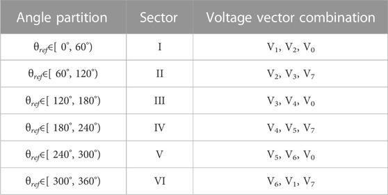
TABLE 1. Voltage vector combination selection.

According to the deadbeat control theory, the predicted current at the moment k+1 is assumed to be as follows:

$\left\{\begin{array}{l}{i}_{dref}=i_d\left(k+1\right)\\ i_{qref}=i_q\left(k+1\right)\end{array}\right.(32)$

Substituting Eq. 32 into Eq. 30), the reference voltages of VSC u_Ndref and u_Nqref can be written as:

$\left\{\begin{array}{l}{u}_{Ndref}=\frac{L}{T_s}\left[i_d\left(k\right)-i_{dref}\right]-R{i}_d\left(k\right)+{\omega }_{1}L{i}_q\left(k\right)+u_d\left(k\right)\\ u_{Nqref}=\frac{L}{T_s}\left[i_q\left(k\right)-i_{qref}\right]-R{i}_q\left(k\right)-{\omega }_{1}L{i}_d\left(k\right)+u_q\left(k\right)\end{array}\right.(33)$

5.2.1 Sector selection

The u_Ndref and u_Nqref are dq0-αβ transformed to obtain the reference voltages of u_Nαref, u_Nβref in αβ coordinates. The phase angle θ_ref of the reference voltage can be calculated as follows:

${\theta }_{ref}=\arctan \left(\frac{u_{N\alpha ref}}{u_{N\beta ref}}\right)(34)$

According to the phase angle shown in Table 1, the sector and vector are selected. By judging the sector, a zero vector (u_0opt) and two non-zero vectors (u_1opt, u_2opt) are determined.

As shown in Figure 6, if the θ_ref of the derived reference voltage vector V_ref falls in the first sector, the corresponding switching state (100) is the optimal switching state. When selecting the voltage zero vector as the optimal voltage vector, both switching states (000) and (111) can generate the voltage zero vector. However, one of the switching states in (000) and (111) should be selected based on the principle of the minimum switching frequency. If the previous switching state was (100), the current switching state should be selected as (000). If the previous switching state was (110), the current switching state should be selected as (111) (Wang et al., 2021b).

FIGURE 6

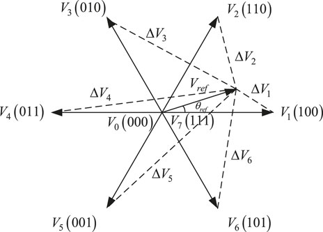
FIGURE 6. Voltage vector selection in the steady-state αβ coordinate system.

5.2.2 Action time calculation

For the determined optimal vector combinations u_0opt, u_1opt and u_2opt, the action time of each vector in the sampling period T_s needs to be calculated. According to the modulation MPC principle, the action time of the vector is inversely proportional to the cost function. The cost function uses Eq. 31. The time of voltage vectors T₀, T₁ and T₂ can be calculated as:

$\left\{\begin{array}{l}{T}_0=\frac{f_1{f}_2}{f_0{f}_1+f_0{f}_2+f_1{f}_2}{T}_s\\ T_1=\frac{f_0{f}_2}{f_0{f}_1+f_0{f}_2+f_1{f}_2}{T}_s\\ T_2=\frac{f_0{f}_1}{f_0{f}_1+f_0{f}_2+f_1{f}_2}{T}_s\end{array}\right.(35)$

Where f₀, f₁, and f₂ are the corresponding cost function Eq. 31 values of u_0opt, u_1opt, and u_2opt (Wang et al., 2022). The two ports of the SOP have similar action times, and the voltage combination and action times are output to both sides of the SOP for the control of the whole system. Figure 7 is the block diagram of the ULMFPC with ESO and TV-MPC for SOP.

FIGURE 7

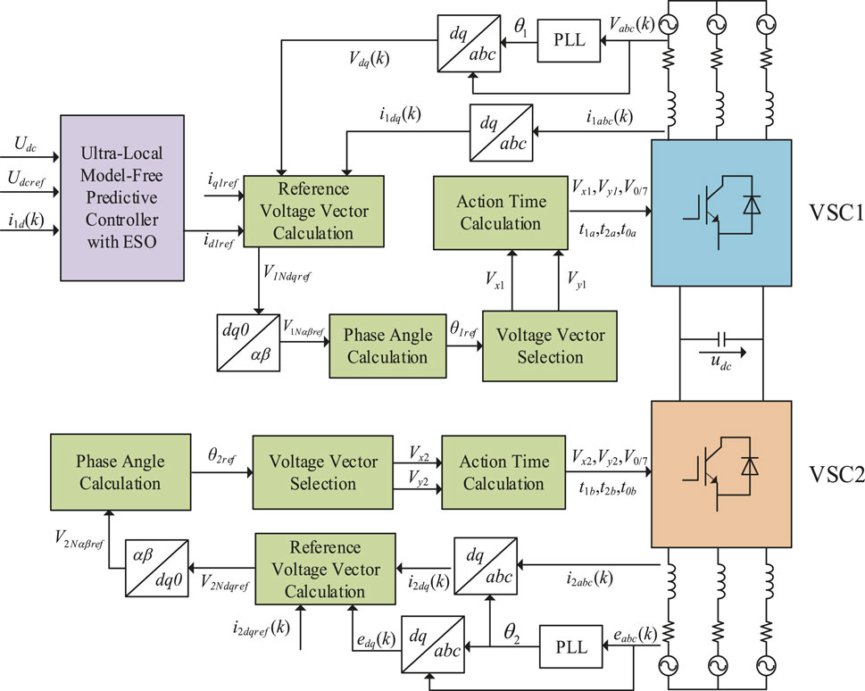
FIGURE 7. Block diagram of the proposed control scheme of SOP.

6 Simulations

In this paper, a control strategy ESO-based ULMFPC and TV-MPC are proposed for the parameter perturbation and current fluctuation of the two-port SOP. The proposed control strategy is simulated and verified based on MATLAB/Simulink. Traditional PI and MPC control strategies are compared with the proposed method to verify the effectiveness of the proposed control strategy. The system parameters of SOP are listed in Table 2, and the controllers design parameters are listed in Table 3, respectively.

TABLE 2

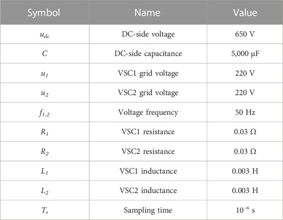
TABLE 2. Parameters of SOP.

TABLE 3

TABLE 3. Controller parameters.

6.1 Performance of steady-state

6.1.1 Current performance of steady-state

The proposed current of the VSC2 side is set as 100 A in simulations. Steady-state currents of PI and MPC, PI and TV-MPC are shown in Figures 8A,B.

FIGURE 8

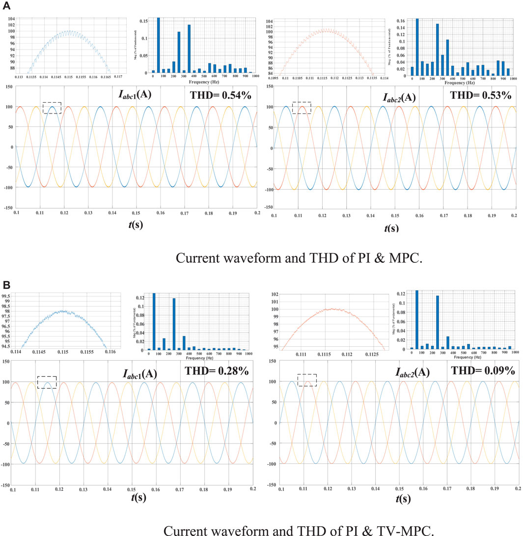
FIGURE 8. (A) Current waveform and THD of PI & MPC. (B) Current waveform and THD of PI & TV-MPC.

It can be seen that the total harmonic distortion (THD) of the A-phase current under PI and MPC control for the VSC1 side and VSC2 side are 0.54% and 0.53%. The THD of the A-phase current under PI and TV-MPC control are 0.28% and 0.09%, respectively. From the experimental results, it can be seen that the proposed TV-MPC method can effectively reduce the total harmonics of the system, but it is less effective in suppressing the 5th order harmonic. Compared with single-vector MPC, TV-MPC have better steady-state current performance.

Figures 9A,B show the d-axis current response on the rectifier VSC1 side. The TV-MPC control strategy is used for the current inner-loop, and the voltage outer-loop is compared with the PI control strategy and the improved ULMFPC control strategy. With no disturbance in the system, i_d1 can track the reference current correctly. It is clearly seen that the output of outer-loop PI controller contains large jitter. But the output i_d1 of the improved ULMFPC controller is smooth, and the tracking time of the specified i_d1ref is much less than that of PI controller, which has better start-up performance.

FIGURE 9

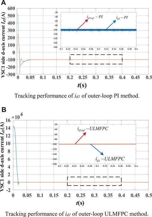
FIGURE 9. (A) Tracking performance of i_d1 of outer-loop PI method. (B) Tracking performance of i_d1 of outer-loop ULMFPC method.

6.1.2 Load power performance of steady-state

Figures 10A,B show the active and reactive power of the load grid under the traditional control strategy and improved control strategy. With no disturbance in the system, two control methods stabilize the load active and reactive power at the specified values. However, the active and reactive power jitter under the ULMFPC with ESO and TV-MPC control are smaller than that of the conventional PI and MPC controllers. And the improved composite control strategy reduces the amplitude of power jitter and improves the response speed effectively.

FIGURE 10

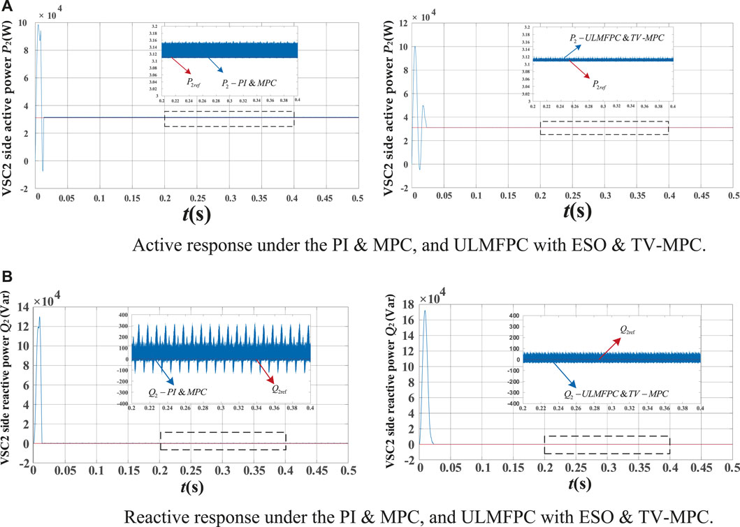
FIGURE 10. (A) Active response under the PI & MPC, and ULMFPC with ESO & TV-MPC. (B) Reactive response under the PI & MPC, and ULMFPC with ESO & TV-MPC.

6.1.3 DC voltage performance

Regulating the proposed DC-side voltage u_dcref at 650 V, in order to verify the effectiveness of ULMFPC with ESO and TV-MPC in start-up response and dynamic performance, the reference current on the VSC2 side is changed from 100 A to 50 A at 0.25 s. As shown in Figure 11, the time used to track the proposed DC voltage under PI and TV-MPC, ULMFPC with ESO and TV-MPC are 0.057 and 0.029 s. From the experimental results, it is observed that ULMFPC with ESO track the proposed DC voltage faster than PI controller, which have better start-up response performance.

FIGURE 11

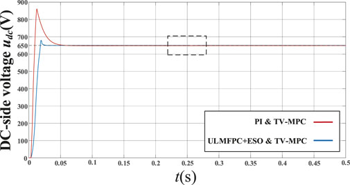
FIGURE 11. DC-side voltage waveform of PI & TV-MPC, and ULMFPC with ESO & TV-MPC.

6.2 Performance of transient-state

6.2.1 Anti-interference performance of DC voltage

In order to verify the good dynamic performance and robustness of the proposed control method, the load grid current is changed from 100 A to 50 A at 0.25 s, and the DC-side voltage variation is shown in Figure 12. It can be seen that the recovery time used to track the DC-side voltage and voltage drop of ULMFPC with ESO and TV-MPC are much smaller than that of PI and TV-MPC. The results show that ULMFPC with ESO have better performance in terms of starting response and response to voltage change.

FIGURE 12

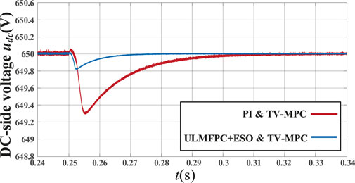
FIGURE 12. Detailed view of Figure 10 in dynamic state.

6.2.2 Current performance of transient-state

The load grid current changes at 0.25 s, and the change of the current on the VSC1 side are shown in Figures 13A,B.

FIGURE 13

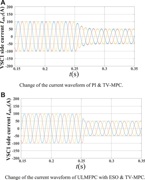
FIGURE 13. (A) Change of the current waveform of PI & TV-MPC. (B) Change of the current waveform of ULMFPC with ESO & TV-MPC.

It can be seen that the recovery of the current under PI and TV-MPC control are significantly weaker than that of the ULMFPC with ESO and TV-MPC control methods. The results show that ULMFPC with ESO have good performance in response speed and current change response.

Figure 14 shows the d-axis current response on the VSC1 side. The reference currents are accurately tracked in the case of abrupt changes on the load side of the system. It can be clearly seen that the PI and TV-MPC controllers take a longer time for i_d1 to recover to the specified value. In contrast, the improved ULMFPC and TV-MPC controllers take much less time to track the specified i_d1ref than the PI and TV-MPC controllers. Thus, the improved control method has a faster tracking performance.

FIGURE 14

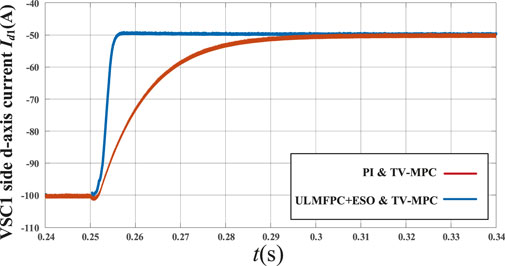
FIGURE 14. Change of i_d1 waveform of PI & TV-MPC, and ULMFPC with ESO & TV-MPC.

6.2.3 Load power performance of transient-state

The response to sudden changes in active and reactive power of the load grid under two composite control methods are shown in Figures 15A,B. Two composite control methods are able to stabilize the load active and reactive power at the specified values without disturbances. However, when power fluctuations occur, the improved ULMFPC and TV-MPC controllers have better recovery tracking performance. The active power can be restored to stability and maintained quickly. And the reactive power can be reset to zero in a shorter time.

FIGURE 15

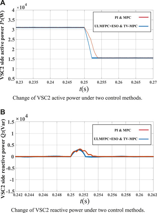
FIGURE 15. (A) Change of VSC2 active power under two control methods. (B) Change of VSC2 reactive power under two control methods.

7 Future work and conclusion

For the better performance of the SOP system, considering access to energy storage and other devices, considering the faults that may occur in the system, taking control strategy under different working modes into consideration, and a semi-physical experimental study of the SOP system will be the future work.

In this paper, an extended state observer-based predictive control method for SOP system is proposed to improve the anti-interference and robustness of the rectifier-side and inverter-side controllers of SOP. The parameter sensitivity problem in the SOP system is analysed. In order to address the parameter ingestion problem, the outer-loop adopts an ultra-local model-free voltage prediction method, which effectively reduces the sensitivity of the parameters. The ESO is established to observe the total system disturbance and perform compensation for the delay existing in the digital control system, which improves the robustness of the SOP system to disturbances. The current TV-MPC method is adopted in the inner-loop to improve the current harmonics effectively. From the simulation results be seen that the total harmonic distortion (THD) of the A-phase current under MPC control for the VSC1 side and VSC2 side are 0.54% and 0.53%. The THD of the A-phase current under TV-MPC control are 0.28% and 0.09%, respectively. Compared with the traditional PI and MPC control strategies, the simulation results show that the control strategies of ULMFPC with ESO and TV-MPC can effectively reduce the current harmonics. and the DC voltage has a better operation, which proves the effectiveness and correctness of the proposed method.

Data availability statement

The original contributions presented in the study are included in the article/Supplementary Material, further inquiries can be directed to the corresponding author.

Author contributions

ZW: Conceptualization, algorithm innovation, methodology, and writing—original draft; PL: Data and formal analysis, investigation, software, simulation, and writing—original draft; HZ: Formal analysis, and writing—review and editing; LC: Formal analysis, and writing—review and editing; All authors have read and agreed to the published version of the manuscript.

Acknowledgments

The authors would like to express their gratitude to all those who helped them during the writing of this paper. The authors would like to thank the reviewers for their valuable comments and suggestions.

Conflict of interest

The authors declare that the research was conducted in the absence of any commercial or financial relationships that could be construed as a potential conflict of interest.

Publisher’s note

All claims expressed in this article are solely those of the authors and do not necessarily represent those of their affiliated organizations, or those of the publisher, the editors and the reviewers. Any product that may be evaluated in this article, or claim that may be made by its manufacturer, is not guaranteed or endorsed by the publisher.

References

Cai, Y., Qu, Z., Yang, H., Zhao, R., Lu, Y., and Yang, Y. (2018). “Research on an improved droop control strategy for soft open point,” in Proceedings of the 2018 21st international conference on electrical machines and systems (Jeju, Korea: ICEMS), 2000–2005.

CrossRef Full Text | Google Scholar

Cao, W., Wu, J., Jenkins, N., Wang, C., and Green, T. (2016). Operating principle of soft open points for electrical distribution network operation. Appl. Energy. 164, 245–257. doi:10.1016/j.apenergy.2015.12.005

CrossRef Full Text | Google Scholar

Chi, R., Yu, H., Zhang, S., Huang, B., and Hou, Z. (2020). Discrete-time extended state observer-based model-free adaptive control via local dynamic linearization. IEEE Trans. Industrial Electron. 67 (10), 8691–8701. doi:10.1109/TIE.2019.2947873

CrossRef Full Text | Google Scholar

Falkowski, P., and Sikorski, A. (2018). Finite control set model predictive control for grid-connected ac–dc converters with lcl filter. IEEE T Rans. Ind. Electron. 65 (4), 2844–2852. doi:10.1109/TIE.2017.2750627

CrossRef Full Text | Google Scholar

Gong, J., Dang, D., and Li, Y. (2021). “Research on key technologies of SNOP suitable for distribution network,” in Ieee. Int. Conf. Circuits and systems (ICCS) (Chengdu, China: IEEE). doi:10.1109/ICCS52645.2021.9697302

CrossRef Full Text | Google Scholar

Huo, Y., Li, P., Ji, H., Yan, J., Song, G., Wu, J., et al. (2021). Data-driven adaptive operation of soft open points in active distribution networks. IEEE Trans. Ind. Appl. 17 (12), 8230–8242. doi:10.1109/TII.2021.3064370

CrossRef Full Text | Google Scholar

Hur, N., Jung, J., and Nam, K. (2001). A fast dynamic DC-link power-balancing scheme for a PWM converter-inverter system. IEEE Trans. Ind. Electron. 48 (4), 794–803. doi:10.1109/41.937412

CrossRef Full Text | Google Scholar

Li, B., Liang, Y., Wang, G., Li, H., and Ding, J. (2020). A control strategy for soft open points based on adaptive voltage droop outer-loop control and sliding mode inner-loop control with feedback linearization. Int. J. Electr. Power & Energy Syst. 122, 106205. doi:10.1016/j.ijepes.2020.106205

CrossRef Full Text | Google Scholar

Li, Z., Hao, Q., Gao, F., Wu, L., and Guan, M. (2019). Nonlinear decoupling control of two-terminal MMC-HVDC based on feedback linearization. IEEE Trans. Power Deliv. 34 (1), 376–386. doi:10.1109/TPWRD.2018.2883761

CrossRef Full Text | Google Scholar

Liang, X., Saaklayen, M. A., Igder, M. A., Shawon, S. M. R. H., Faried, S. O., and Janbakhsh, M. (2022). Planning and service restoration through microgrid formation and soft open points for distribution network modernization: A review. IEEE Trans. Ind. Appl. 58 (2), 1843–1857. doi:10.1109/TIA.2022.3146103

CrossRef Full Text | Google Scholar

Liu, K., and Gao, L. (2020). Improved model of predictive direct torque control for permanent magnet synchronous motor. Electr. Mach. Control 24 (1), 10–17. doi:10.15938/j.emc.2020.01.002

CrossRef Full Text | Google Scholar

Liu, X., Li, K., and Zhang, Q. (2018). Single-loop predictive control of PMSM based on nonlinear disturbance observers. Proc. CSEE 38 (7), 2153–2162. doi:10.13334/j.0258-8013.pcsee.170554

CrossRef Full Text | Google Scholar

Morsi, A., Abbas, H. S., Ahmed, S. M., and Mohamed, A. M. (2021). Model predictive control based on linear parameter-varying models of active magnetic bearing systems. IEEE Access 9, 23633–23647. doi:10.1109/ACCESS.2021.3056323

CrossRef Full Text | Google Scholar

Morsi, F., and Cedric, J. (2021). “Defense against DoS and load altering attacks via model-free control: A proposal for a new cybersecurity setting,” in 5th int. Conf. Control and fault-tolerant systems (SysTol) (Saint-Raphael, France: IEEE). doi:10.1109/SysTol52990.2021.9595717

CrossRef Full Text | Google Scholar

Rodriguez, J., Pontt, J., Silva, C., Correa, P., Lezana, P., Cortes, P., et al. (2007). Predictive current control of a voltage source inverter. IEEE Trans. Ind. Electron. 54 (1), 495–503. doi:10.1109/TIE.2006.888802

CrossRef Full Text | Google Scholar

Rueda, M., and Padilha, F. (2013). Distributed generators as providers of reactive power support—A market approach. IEEE Trans. Power Syst. 28 (1), 490–502. doi:10.1109/TPWRS.2012.2202926

CrossRef Full Text | Google Scholar

Pamshetti, V., Singh, S., Thakur, A. K., and Singh, S. P. (2021), Multistage coordination Volt/VAR control with CVR in active distribution network in presence of inverter-based DG units and soft open points. IEEE Trans. Ind. 57 (3). 2035–2047. doi:10.1109/TIA.2021.3063667

CrossRef Full Text | Google Scholar

Wang, X., and Li, H. (2021). “A deadbeat modulated model-free predictive current control of SMPMSM drive system,” in 12th IEEE. Conf. Energy conversion congress & exposition-asia (ECCE-Asia) (Singapore, Singapore: IEEE). doi:10.1109/ECCE-Asia49820.2021.9479321

CrossRef Full Text | Google Scholar

Wang, Z., Sheng, L., Huo, Q., and Hao, S. (2021). An improved model predictive control method for three-port soft open point. Math. Probl. Eng. 2021, 9910451. doi:10.1155/2021/9910451

CrossRef Full Text | Google Scholar

Wang, Z., Zhao, X., and Guo, Y. (2021). “Three-vector predictive current control for interior permanent magnet synchronous motor,” in Ieee. Int. Conf. Predictive control of electrical drives and power electronics (PRECEDE) (Jinan, China: IEEE). doi:10.1109/PRECEDE51386.2021.9680998

CrossRef Full Text | Google Scholar

Wang, Z., Zhou, H., and Su, H. (2022). Disturbance observer-based model predictive super-twisting control for soft open point. Energies 2022 (15), 3657–57. doi:10.3390/en15103657

CrossRef Full Text | Google Scholar

Wu, R., Ran, L., Weiss, G., and Yu, J. (2018). Control of a synchronverter-based soft open point in a distribution network. J. Eng. 2019 (16), 720–727. doi:10.1049/JOE.2018.8382

CrossRef Full Text | Google Scholar

Jiang, X., Zhou, Y., Ming, W., Yang, P., and Wu, J. (2022). An overview of soft open points in electricity distribution networks. IEEE Trans. Smart Grid 13 (3), 1899–1910. doi:10.1109/TSG.2022.3148599

CrossRef Full Text | Google Scholar

Xu, L., Chen, G., Li, G., and Li, Q. (2020). Model predictive control based on parametric disturbance compensation. Math. Probl. Eng. 2020, 1–13. doi:10.1155/2020/9543928

CrossRef Full Text | Google Scholar

Yang, S., Wang, Y., and Chu, Z. (2020). Current decoupling control of PMSM based on an extended state observer with continuous gains. Proc. CSEE 40 (6), 1985–1997. doi:10.13334/j.0258-8013.pcsee.191226

CrossRef Full Text | Google Scholar

Young, H., Perez, M., and Rodriguez, J. (2016). Analysis of finite-control-set model predictive current control with model parameter mismatch in a three-phase inverter. IEEE Trans. Ind. Electron. 63 (5), 3100–3107. doi:10.1109/TIE.2016.2515072

CrossRef Full Text | Google Scholar

Zhang, G., Hou, L., and Peng, B. (2020). Feedback linearization sliding mode control strategy for soft open point. Automation Electr. Power Syst. 44 (1), 126–133. doi:10.7500/AEPS20190616005

CrossRef Full Text | Google Scholar

Zhang, G., Peng, B., and Xie, R. (2018). Predictive synergy control strategy for flexible multi-state switch model. Automation Electr. Power Syst. 42 (20), 123–136. doi:10.7500/AEPS20180210002

CrossRef Full Text | Google Scholar

Zhang, H., Zhang, Y., and Liu, J. (2017). Model-free predictive current control of permanent magnet synchronous motor based on single current sampling. Trans. China Electrotech. Soc. 32 (2), 180–187. doi:10.19595/j.cnki.1000-6753.tces.2017.02.021

CrossRef Full Text | Google Scholar

Zhang, X., Zhang, L., and Zhang, Y. (2019). Model predictive current control for pmsm drives with parameter robustness improvement. IEEE Trans. Power Electron. 34 (2), 1645–1657. doi:10.1109/TPEL.2018.2835835

CrossRef Full Text | Google Scholar

Zhang, Y., Yin, Z., Li, W., and Liu, J. (2021). Adaptive sliding-mode-based speed control in finite control set model predictive torque control for induction motors. IEEE Trans. Power Electron. 36 (7), 8076–8087. doi:10.1109/TPEL.2020.3042181

CrossRef Full Text | Google Scholar

Zhang, Z., Fang, H., Gao, F., Rodríguez, J., and Kennel, R. (2017). Multiple-vector model predictive power control for grid-tied wind turbine system with enhanced steady-state control performance. IEEE Trans. Power Electron. 64 (8), 6287–6298. doi:10.1109/TIE.2017.2682000

CrossRef Full Text | Google Scholar

Zhou, Y., Li, H., and Yao, H. (2016). “Model-free control of surface mounted PMSM drive system,” in Int. Conf. Industrial technology (ICIT) (Taipei, Taiwan: IEEE). doi:10.1109/ICIT.2016.7474746

CrossRef Full Text | Google Scholar