An electricity load forecasting model based on multilayer dilated LSTM network and attention mechanism

1 Introduction

As a special kind of secondary energy, the most prominent feature of electricity is the simultaneity, or the complete synchronization of electricity generation by power plants and consumption by consumers. Because it is difficult to achieve a large amount of storage for electricity, the best way is to ensure the efficient operation of the power grid is to maintain the power generation and electricity consumption in a dynamic equilibrium state at all times. To forecast power load for a future period, load forecasting analyzes past information data, such as power load, weather change, economic development, etc. It can assist in optimizing control unit operation, reducing power generation costs, and improving economic efficiency. Load forecasting can be divided into long-term, medium-term, short-term, and ultra-short-term according to the projected time span (Hussain et al., 2021). Ultra-short term typicallyrefers to load forecasting for the next few hours (Khan et al., 2016). Accurate forecasting is important to the adjustment efforts of power generation companies and the scheduling of power grids. Load data is a non-linear time series, and electricity load forecasting methods are classified into the following categories: time series analysis, machine learning, and neural network.

Exponential smoothing (Smyl, 2020), auto-regressive moving average model (ARIMA) (Wei and Zhen-gang, 2009; Kim et al., 2019), among others, are examples of forecasting methods based on time series analysis. These methods mainly apply and analyze the laws of mathematical statistics and stochastic process theory to predict the system’s future development trend. However, this type of methods have good prediction accuracy only for load series with low fluctuation, and it can only be used for single variable prediction. It cannot be used effectively when other related variables such as weather and date exist. To analyze the impact on load data of multiple factors, multivariate load forecasting is addressed using machine learning-based methods such as Support Vector Machines (SVM) (Paudel et al., 2017; Aasim et al., 2021), Random Forest (Bogomolov et al., 2016; Li et al., 2020), and XGBoost (Wang et al., 2021a; Dai et al., 2022). These models are capable of automatically learning not only the series’ more complex features, but also the non-linear relationship between some factors and load data. However, the overreliance of these methods on sample selection of similar data makes the model construction and update processes inflexible, and the load forecasting accuracy cannot meet the requirements of modern power systems.

Neural networks have the associative memory function and the ability of parallel information distribution, self-learning, and arbitrary approximation of continuous functions, which enables them to capture various changes of electricity load and analyze non-linear relationships between load data and other data. The simplest and most basic neural network model is the multilayer perceptron (MLP) (Hernandez et al., 2014; Mohammed and Al-Bazi, 2022; Pavićević and Popović, 2022), which consists of fully connected neurons. Load and related data are propagated forward in the multilayer perceptron, and parameters are optimized through error backpropagation (BP) (Su et al., 2017; Qiao, 2018) to produce a predicted output that progressively approximates the true load. By using clustering analysis to classify different loads on big data platforms, Su et al. (Su et al., 2017) improved prediction accuracy using multiple BP neural networks to solve the time consuming and overfitting problems in big data. Based on the concept of simulated annealing, Qiao (2018) proposed a method that combines particle swarms optimization algorithm with the BP algorithm (SAPOS-BP) for electricity load forecasting. This method improved the generalization and self-learning ability of the model. Combining wavelet decomposition techniques with neural networks, Rana and Koprinska (2016) proposed an advanced neural network for short-term load forecasting.

The recurrent neural network (RNN) (Yang et al., 2019) is a common method to deal with time series problems. It has good time series information extraction and non-linear learning abilities, and it can simultaneously learn the influence of other factors (such as weather, date, etc.) on load data. The long short-term memory neural network (LSTM) is a special type of RNN and can overcome the shortcomings of the vanishing gradient and gradient explosion in conventional RNN. It is widely used in natural language processing (NLP), language translation and sequence prediction. Islam et al. (2023) used a hybridization model of RNN and LSTM for sentiment analysis of user ratings in an online meeting app. Yang (2022) applied LSTM to the field of intelligent translation of English. Peng et al. (2022) employed LSTM in energy consumption forecasting to achieve a better prediction performance and the more critical influencing factors are emphasized. Due to its good time series processing capabilities, LSTM has also found many applications for load forecasting studies. LSTM was used in (Ciechulski and Osowski, 2021) to predict 24 and 1 h on two load datasets respectively, showing good forecasting ability and applicability. Li et al. (2023) constructed a CEEMDAN-SE-LSTM model based on time series decomposition-reconstruction modeling and neural network forecasting. The Gated Recurrent Unit (GRU) is a variant of LSTM, with a simpler structure and a common time-series processing network. Mahjoub et al. (2022) compared LSTM, GRU, and Drop-GRU networks with the ability to prevent overfitting in the same environment and showed that LSTM had the best load forecasting effect. Bidirectional long short-term memory (Bi-LSTM) is an extension of the conventional LSTM, which can learn from both ends of the sequence at the same time. Siami-Namini et al. (2019) demonstrated the model’s usability in load prediction and showed that is has superior ability compared to conventional LSTM. In Guo et al. (2022) proposed a combined load forecasting method for Multi-Energy System (MES) based on Bi-directional Long Short-Term Memory (BiLSTM) multi-task learning. In recent years, the combination of convolutional neural networks (CNNs) (Khan et al., 2019; Imani, 2021) and recurrent neural networks has gained popularity. The main idea is to use CNN to extract spatial information in the series, and then extract the time information by LSTM, which can not only increase the amount of learned information but also produce better predictions than a single network. A combination of deep residual neural network and stacked LSTM for building load forecasting was used in (Khan et al., 2022). Wang et al. (2021b) combined CNN and BiLSTM for electricity load forecasting. These hybrid prediction methods have demonstrated superior performance over a single LSTM network. Echo state network (ESN) is another unique RNN. A modified hybrid model was used by Peng et al. (2021) called improved backtracking search optimization algorithm (IBSA)–double-reservoir echo state network (DRESN) (IBSA–DRESN) for effective electricity load forecasting.

Attention mechanisms have gained a lot of attention on speech recognition, image recognition, machine translation, and many other fields in recent years. Attention has a strong ability to capture key information, and it was applied for some studies to improve the accuracy of load forecasting. In Jung et al. (2021) constructed an attention-based multilayer GRU model for building load prediction an hour in advance, and showed that this method significantly improved forecasting accuracy compared to the underlying GRU. Wu et al. (2021) combined the attention mechanism with CNN to extract the spatial characteristics of the data and used LSTM and BiLSTM to extract the time information to effectively predict the power load in the integrated energy system. The Sequence to Sequence (Seq2Seq) architecture (Sutskever et al., 2014; Gong et al., 2019) was first applied in the field of Natural Language Processing (NLP) (Kwon, 2019) and has also been used for short-term load forecasting in recent years. It is divided into two parts: encoder and decoder. The encoder extracts the information from the input series and compresses it into a fixed context vector. The context vector, which is rich in historical load information, is then decoded by the decoder into the desired value. The lengths of its input and output series are variable and can be different. Du et al. (2020) designed an end-to-end structure based on the attention mechanism and Sequence to Sequence model to address the issue of multivariate time series forecasting, and verified it on five multivariate time series datasets. In (Sehovac and Grolinger, 2020), load forecasting performance was compared between multiple RNN cells (vanilla, LSTM, GRU) and different attention mechanisms [Bahdanau (Bahdanau et al., 2014) attention (BA), Luong (Luong et al., 2015) attention (LA)] in the Seq2Seq framework, and experiments showed that seq2seq with BA had the best overall prediction performance.

The most commonly used method in the field of series forecasting is still recurrent neural network and has been used with good results of many studies. Most of the existing load forecasting methods use LSTM network or mixed network model. This raises two issues: one of them is that although LSTM networks alleviate to a certain extent the drawback of traditional RNN networks that cannot handle long series, the scope of their attention is still limited. Generally speaking, for series with orders of magnitude less than 100, LSTM networks can perform the task of serial forecasting relatively well. Beyond this limit, the forecasting accuracy of the LSTM network will be decreasing. Secondly, in serial forecasting the input and output dimensions are often unequal, which requires the use of Seq2Seq models to map them. One of the two: in serial forecasting the input and output dimensions are often unequal, which requires the use of Seq2Seq model to map them. However, Seq2Seq has the generation of context vectors, which will lose the series information extracted by the Encoder layer to some extent, making the forecasting accuracy lower.

To solve the above problems, we first used multilayer dilated LSTM networks instead of traditional LSTM network as the Encoder layer. Dilated LSTM networks not only preserve longer memories in long series, but their multilayer structure enables the extraction of series information in different dimensions. Secondly, to reduce the loss of information when context vectors are generated, we used an attention mechanism that focuses it more of the important information in the original series and can reduce the interference in cluttered information. We proposed a hybrid model based on the Seq2Seq framework that combines dilated LSTM networks, attentional mechanism, and LSTM networks for electricity load forecasting using long series. The model uses a multilayer dilated LSTM (Chang et al., 2017) structure as the encoder layer, which learns non-linear and multidimensional dependencies on long load series. The encoder layer’s output is expressed using an attention mechanism to reduce the influence of redundant information on the subsequent decoding process. Finally, a single-layer LSTM network is used to decode the data, and the output load of the full-connection layer is used to forecast the result. The contributions of this paper are as follows:

(1) We used a multilayer extended LSTM network instead of traditional LSTM to extend the length of the historical series in load forecasting.

(2) In order to improve the accuracy of load forecasting, a new model has been established. This model uses a multilayer dilated LSTM structure as Encoder layer to extract long series information under the Seq2Seq framework, introduces attention mechanism to focus on key information, and finally LSTM are employed to decode the context vectors.

(3) Experiments have been conducted on two real load datasets in different regions, and the results show that the proposed model has a higher forecasting accuracy compared to the benchmark methods.

The rest of the paper is organized as follows: Section 2 introduces some related models and frameworks, Section 3 describes the methodology, Section 4 shows the data selection and preprocessing, Section 5 explains the experiments and corresponding results, and at Section 6 concludes the paper.

2 Related theories

2.1 LSTM

RNN is mainly used in series data processing. It remembers previous information and uses that information to influence the output of subsequent nodes. However, basic RNN networks are not only prone to the vanishing gradient and gradient explosion issues, but also do not effectively handle “long-distance dependency.” LSTM (Staudemeyer and Morris, 2019) is a variant of RNN, proposed by Hochreiter and Schmidhuber (1997) in 1997. Its emergence has largely addressed the shortcomings of the classic RNN, which has been later improved and promoted by many scholars.

The LSTM network added cell states representing long-term information to the original RNN hidden state. The structure of an LSTM cell includes an input gate, an output gate, a forget gate, and a cell state, as shown in Figure 1. Each LSTM cell receives three inputs: input vector x_t, hidden state h_t−1, and previous cell state c_t−1. It also has two outputs: hidden state h_t and the current cell state c_t.

FIGURE 1

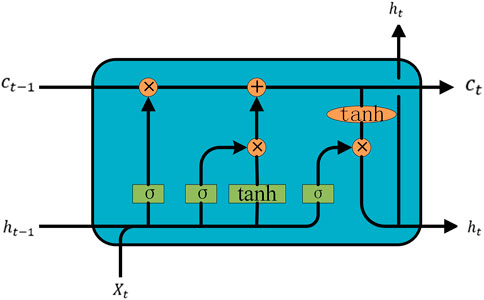
FIGURE 1. Cell structure of LSTM.

The forget gate takes the input vector x_t and hidden state h_t−1 of the previous neuron as input, indicating the extent to which information was forgotten in the previous neuron, expressed as:

$f_t=\sigma \left(W_i\left[h_{t-1},x_t\right]+b_i\right)(1)$

The update gate is mainly to retain the total information of the new input x_t first, and then update the cell state:

$u_t=\sigma \left(W_j\left[h_{t-1},x_t\right]+b_j\right)(2)$

$v_t=tanh\left(W_z\left[h_{t-1},x_t\right]+b_z\right)(3)$

$c_t=f_t*c_{t-1}+u_t*v_t(4)$

The output gate is to fuse the input of this cell with the information of the previous cell to form a new series information.

$y_t=\sigma \left(W_o\left[h_{t-1},x_t\right]+b_o\right)(5)$

$h_t=y_t*tanh\left(c_t\right)(6)$

W_x and b_x(x = i, j, z, o) are the weight parameters and bias of the model, respectively. Their initial values are usually randomly generated and shared among the weight of each layer of the network to prevent the gradient from exploding or vanishing. σ(x) is the Sigmoid activation function, $\sigma (x)={(1+e^{-x})}^{-1}$, and tanh(x) is the hyperbolic tangent activation function. The initial parameters of the hidden layer are randomly generated in [0, 1]. As the network is trained, the Adam method is used to gradually update the parameters in the LSTM network by back-propagation of errors, so that the whole model achieves the desired forecasting results.

2.2 Dilated LSTM

The LSTM network receives time series data sequentially and can memorize information in long series by hiding states and cell states. The left subgraph in Figure 2 shows a layer of conventional LSTM structure, where information is transmitted sequentially between different nerve cells within a layer, and h_t and c_t of one neuron can only be transmitted to the next cell. However, this type of memory is only a short-distance long-term memory. Due to parameter limitations, the hidden state information, which has the function of memory, will always be replaced by the new information. Therefore, when the length of the sequence is relatively long, the front-end information on the sequence is not well preserved. This is somewhat mitigated by the Dilated RNN structure (Chang et al., 2017; Smyl et al., 2021), whose network structure is shown on the right of Figure 2. Its most notable feature is the multiresolution expansion loop jump, which can not only alleviate gradient problems but also expand the dependencies with fewer parameters. Using a multilayer expansion loop layer can also learn dependencies on multiple dimensions.

FIGURE 2

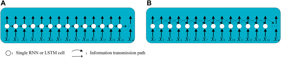
FIGURE 2. Basic (A) and dilated (B) LSTM Network.

In the Dilated LSTM structure, a cell in the same layer does not receive h_t−1 and c_t−1 from the previous cell, but rather the output information h_t−d and c_t−d in the previous d (d = 2 in Figure 2) cell, thereby obtaining the information dependence of long time series. This structure has two benefits: first, it allows different layers to focus on different dimensions of time, and second, the average length between timestamps is reduced. Not only can the ability of LSTM to extract long-distance dependencies be improved, but the vanishing gradient and gradient explosion can also be prevented.

2.3 Seq2Seq model

The Seq2Seq model can be specifically used to deal with variable-length time series problems under the Encoder-Decoder framework. It consists of three parts, the Encoder part can transform the time series into context vector, which can be decoded into the desired output sequence through the Decoder part. At this point, the output’s length and dimension can be different from the input. The Seq2Seq structure is depicted in Figure 3. Both the Encoder and Decoder modules can use common networks such as CNN, RNN, and LSTM. In load forecasting, we need to use historical load, weather, and date data, among others, to forecast the load for a period of time in the future. The Seq2Seq model can achieve this goal effectively.

FIGURE 3

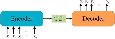
FIGURE 3. Seq2Seq architecture.

2.4 Attention mechanism

When using the Seq2Seq model, the Encoder module transforms the input time series into a fixed-length context vector after learning. However, the generation of context vectors is the result of data compression, which inevitably results in information loss. Using the attention mechanism can assign different weights to different features so that important information receives more attention. Therefore, since the output of the conventional encoder is a single long tensor and cannot store too much information, this paper proposes to use the attention mechanism in the Encoder module, which can effectively focus the output results of the encoder according to the target. Since the time series has been processed, the information remembered by the Encoder can be directly treated as the initial hidden layer of the Decoder. The computational steps of the attention mechanism include the following:

2.4.1 Calculate weights

$W_i=h_i*S^T(7)$

where h_i represents the state of the last hidden Encoder layer at times i, S is the last hidden state, numerically the same as h_m and *denotes the multiplication of two tensors. W_i denotes the correlation weight between S and h_i. To better represent the different levels of importance in the initial series, the hidden states at different moments are multiplied with the final state vector to represent their attention probability distribution values. The weights W_i are recalculated during each training session.

2.4.2 Normalization of weight vectors

$a_i=\frac{exp\left(W_i\right)}{\sum _{i=1}^{m}exp\left(W_i\right)}(8)$

where a_i is the result of normalizing the weight vector W_i.

2.4.3 Calculating attention

$c_0=\sum _{i=1}^m{a}_i{h}_i(9)$

The calculation of c₀ considers the hidden layer h_i(i = 1, 2, 3, …, m) at all times, which is denoted by the input sequence X. That is to say, c₀ takes all inputs into account, and with the attention mechanism, it gives more attention to important input moments and less attention to others. The structure of the attention mechanism is shown in Figure 4.

FIGURE 4

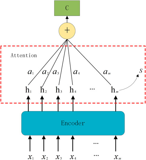
FIGURE 4. Unit structure of attention mechanism.

3 Methodology

3.1 Proposed network architecture

This paper proposes a short-term load forecasting model that combines dilated LSTM and attention mechanism under the Seq2Seq framework. The specific implementation process is shown in Figure 5. First, the collected load data are pretreated with relevant factor data such as date and weather, and split into training, validation, and test datasets. In this model, three different levels of dilated LSTM structure are used as the Encoder layer under the Seq2Seq framework to extract the dependencies in the original long series. Three levels of dilated LSTM are used, namely, d = 2, d = 4, and d = 1. The dilated LSTM of the last layer is equivalent to the basic LSTM network (d = 1), its main function is to aggregate and memorize the information extracted from the first two layers. Training and validation data are fed to the Encoder layer to extract non-linear relationships and multidimensional information from long series. The features obtained by the Encoder layer are then used as input to the attention layer, and the key information are distinguished from a weighted form to form a context vector. One layer of basic LSTM network is used as the Decoder layer to decode the context vector formed by the attention layer and predict the future load data through a layer of fully connected nodes.

FIGURE 5

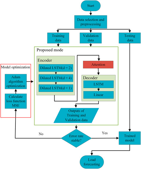
FIGURE 5. Flowchart of the proposed model.

In this paper, other factors related to electricity load, including weather and date, are added to the load forecasting. The data dimension used is high, which makes it less likely that the model has a local minimum. Therefore, it is more important to consider the training convergence of the model. We use the optimization method Adam, which is commonly used in neural networks. This method can not only find the global minima of the model effectively and quickly, but also avoid the training results falling into the local minima to a certain extent. During the training phase, the mean square error (MSE) is calculated as the loss function of the model using the predicted results of the training and validation datasets in the input model with corresponding true label values, and the model parameters are updated using Adam optimization method in turn through the back-propagation. After training, when the error of the model meets the requirements, the trained model parameters are retained. Finally, the test data are input into the trained model to forecast the future load.

3.2 Evaluation indices

To evaluate the performance of the proposed load forecasting model, four quantitative measures were used, including mean absolute percent error (MAPE), root mean square error (RMSE), mean square error (MAE), and mean square error (MSE) (Chai and Draxler, 2014; Moon et al., 2019):

$\text{MAPE}=\frac{1}{n}\sum _{i=1}^n\frac{|y_i-L_i|}{L_i}\times 100(10)$

$\text{RMSE}=\sqrt{\frac{1}{n}\sum _{i=1}^n{\left(y_i-L_i\right)}^2}(11)$

$\text{MAE}=\frac{1}{n}\sum _{i=1}^n|y_i-L_i|(12)$

$\text{MSE}=\frac{1}{n}\sum _{i=1}^n{\left(y_i-L_i\right)}^2(13)$

where L_i is the actual value, y_i is the predicted value, and n is the total number of values. The smaller the value of these four indicators, the smaller the error between the predicted value and the real value, and the more accurate the load forecast.

4 Data selection and preprocessing

4.1 Data selection

To verify the forecasting performance of the proposed model, we selected the true load data (the sampling period is 15 min, MW) of a specific location from January 2020 to August 2022 for experiments. Figure 6A shows the load change curve of the region for 1 year. It can be seen that the change of electricity load is not only related to the date but also to the time of the day. For a more accurate load forecasting, this paper not only considers the date factor, but also includes weather, holidays, and other factors as well. Table 1 lists the various attributes of the dataset used in this work with a brief description of each feature. We used 60% of the total data for training, 20% for validation, and the last 20% for testing.

FIGURE 6

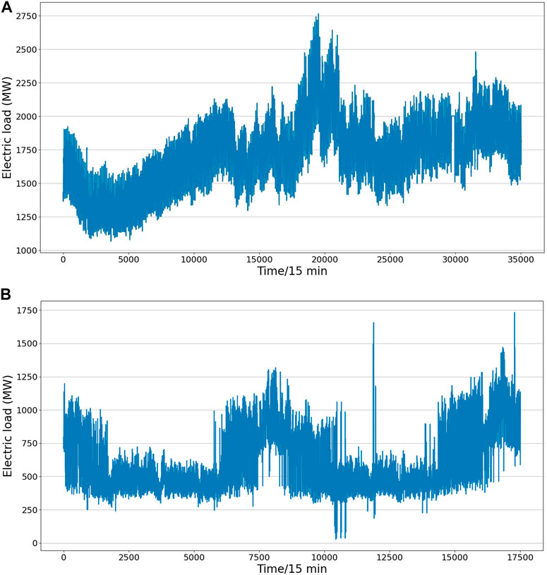
FIGURE 6. Load change curves of two real data. (A) The first place load data, (B) another place load data.

TABLE 1

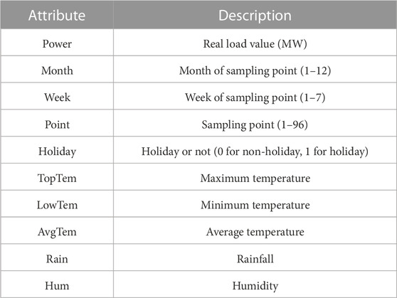
TABLE 1. Dataset features.

4.1.1 Data preprocessing

The obtained load and meteorological data are often subject to data anomalies and deficiencies for several reasons. These anomalies need to be corrected. Load data sampling is continuous, and usually the load does not change much over a continuous period of time. Therefore, when the load difference between two adjacent moments is too large, we consider that there is an anomaly. Consider the following conditions:

$\left\{,\begin{array}{cc}\hfill & |p_i-p_{i-1}|>\zeta \times min\left\{p_i,p_{i-1}\right\},\hfill \\ \hfill & |p_{i+1}-p_i|>\zeta \times min\left\{p_{i+1},p_i\right\},\hfill \end{array}\right.(14)$

where p_i is the load value at time i, and ζ is a threshold between 0 and 1. When p_i meets the above conditions, we determine that it is abnormal and needs to be deleted for subsequent correction. For lost data, prior correction is required. If a single data value is missing, it can be corrected by the nearest average method, expressed as:

$p_i=\left(p_{i+1}+p_{i-1}\right)/2(15)$

When load data are lost for several consecutive days at a certain time, this paper uses the weighted average of the values of the same time of the days before the missing value to replace the next value. Mathematically, it is expressed as:

$p_i=\frac{1}{d}\times \sum _{k=i-d}^{i-1}{W}_k{p}_k(16)$

where w_k(i − d ≤ k ≤ i − 1) is the weight coefficient, and d is the number of days for weighted average. In the case of missing weather data, the above method can also be used when the adjacent weather conditions do not change much. When the missing value differs significantly from the weather before and after, it can be supplemented by replacing the data from the day of the previous year or directly using the data of the previous or following day.

4.2 Data normalization

After processing the anomalous data, the data become relatively smooth, normalization is still required because the units and dimensions of the data are different (Patro and Sahu, 2015). This not only eliminates the influence of different data norms on load forecasting, but also speeds up the convergence of the models and prevents gradient explosion. In this work, the data for each characteristic are normalized into (−1, 1), and the calculation process is as follows:

$\widehat{F}=\frac{F-F_{min}}{F_{max}-F_{min}}(17)$

where F represents the different raw data, $\widehat{F}$ is the normalized data, and F_max and F_min are the maximum and minimum values of the feature, respectively. When the data are preprocessed, time series with different characteristics can be entered into the proposed model for model training and load forecasting.

5 Experimental analysis

The proposed model can effectively extract the non-linear dependencies in quite long series and learn the relevant non-linear relationships from multiple time dimensions. To verify the forecasting performance of the proposed model, we selected two advanced short-term load forecasting methods, LSTM and Seq2Seq, for comparison. LSTM uses a single layer structure, and Seq2Seq uses a layer of LSTM as the Encoder layer and the Decoder layer, respectively. Each time point of the input series in the experiment contains the load value and other characteristics related to the current load, such as:

$\begin{array}{ll}\hfill x_t& =\left\{Power,Month,Week,Point,Holidy,TopTem,LowTem,AvgTem,\right.\hfill \\ \hfill & \left.Rain,Hum\right\}\hfill \end{array}(18)$

To verify the performance of the proposed method under different experimental conditions, we have designed a variety of experiments as follows:

Experiment 1: Load values for the next hour were predicted using a time series from the previous 7 days.

Experiment 2: Load value for the next sampling site were predicted using a time series from the previous 7 days.

Experiment 3: Load values for the next hour were predicted using a time series from the previous 2 days.

5.1 Experimental results

5.1.1 Experiment 1

In the first experiment, the input of the model is the 7 days data in the time series such as {x_t−681, x_t−680, …, x_t−1, x_t}, and the output is 1 h load forecasting (four sampling points {x_t+1, x_t+2, x_t+3, x_t+4}). The results of the four sampling points predicted by the three methods are shown in Figure 7. The horizontal axis represents 150 sample points we selected from the test dataset, and the vertical axis represents load. The two curves are the true and predicted values, respectively. It can be seen that the forecasting curve of the proposed method has a fluctuation closer to the actual load. Figure 8A shows the error curve between the predicted and true values of Figure 7. The curve shown for the proposed method is always between the curves obtained using the other two methods. Overall, the error fluctuates around 0, and the error range is within (−100, 150). It is evident from the forecasting and error curves that the suggested approach is preferable.

FIGURE 7

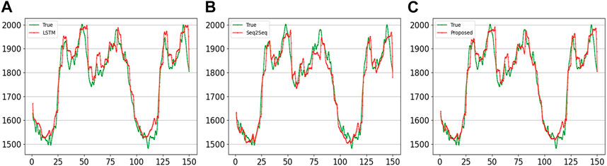
FIGURE 7. Comparison of the curves of four sampling points forecast using 7-day series by different methods. (A) LSTM; (B) Seq2Seq; (C) proposed.

FIGURE 8

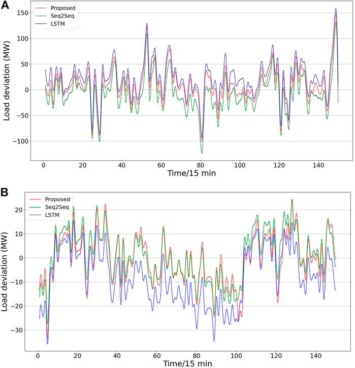
FIGURE 8. Comparison of errors curves using 7-day series by different methods.(A) four sampling points forecasting results, (B) one sampling point forecasting results.

The first three rows in Table 2 shows the indicator results of the four sampling points forecast by different methods. The best value for each index is labeled in bold. The proposed model exhibits better results on the four indicators listed. This shows that the proposed model’s Encoder can effectively extract the information from the long series, while the load of the next hour is more accurately predicted through the Decoder.

TABLE 2

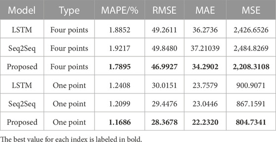
TABLE 2. Index values of four and one sampling points forecast using 7-day series by different methods.

5.1.2 Experiment 2

In the second experiment, we adopt the load series {x_t−681, x_t−680, …, x_t−1, x_t} of the 7 days to predict the load value of the next moment {x_t+1}. Figure 9 displays the results of the forecast curves produced by various methods. The load forecast at the following instant belongs to single step load forecasting, and both Seq2Seq and the proposed method have achieved good forecasting accuracy. Intuitively, there is little difference between the forecast values obtained by the proposed method and the actual values. In the error curve of Figure 8B, the three curves at the left and right ends always fluctuate around 0, and the error of the proposed method basically remains in the middle of the three curves and is closer to 0. However, the curve of the proposed method is always at the highest position around 80. This is because all the forecast values of the three methods are lower than the true values, while the error curve of the proposed method is the closest to 0, and its error range is within (−40, 30).

FIGURE 9

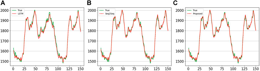
FIGURE 9. Comparison of the curves of next sampling points forecast using 7-day series by different methods. (A) LSTM; (B) Seq2Seq; (C) proposed.

The last three rows in Table 2 shows the indicator results calculated by different methods to forecast load values at the next sampling point. It can be seen that the four indicator values of the proposed method are the smallest, which is consistent with the proposed model’s forecasting error curve being closer to 0. Summarizing the results of experiments 1 and 2, the proposed method outperforms LSTM and Seq2Seq methods in both multistep and single step forecasting.

5.1.3 Experiment 3

Table 3 shows the indicator results from various next hour load forecasting methods using the series data {x_t−191, x_t−190, …, x_t−1, x_t} from the two previous days. It can be seen that the proposed method still outperforms the other two methods in forecasting the next four points using only a 2-day time series. Besides, because the performance of Seq2Seq method is constrained by the length of the context vectors, it exhibits a larger error than that of the LSTM method in load prediction. The performance of the proposed method is the best in load forecasting with a length of 96 × 2, followed by the LSTM method, while the forecasting effect of the Seq2Seq method cannot achieve the expected performance.

TABLE 3

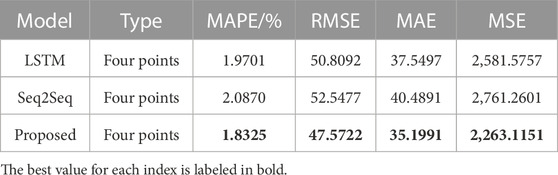
TABLE 3. Index values of four sampling points forecast using 2-day series by different methods.

5.2 Supplementary experiment

In order to better illustrate the generalization and effectiveness of the proposed model, we selected the real load data of a certain year in another place for supplementary experiments. The load sampling points in this data are for 1 h. The load change curve over the course of the year is shown in Figure 6B. Temperature, wind speed and air humidity are the only three factors that have a high correlation with the load selected in order to reduce the effect of too many complex factors. At this time, each time point of the input series in the experiment contains the load value and other characteristics related to the current load, such as:

$y_t=\left\{Power,Temperature,Humidity,Speed\right\}(19)$

In the data preprocessing and specification, we adopt the same method as the previous data. Based on this, we designed the same load forecasting method: use the data of the first 7 days to forecast the load value of the next hour and 4 h respectively.

Figures 10, 11 show the results curves of the different methods using the data series {y_t−167, y_t−166, …, y_t−1, y_t} of 7 days to predict the subsequent 4 h {y_t+1, y_t+2, y_t+3, y_t+4} and 1 h {y_t+1} load values, respectively. It can be seen that the accuracy of different methods in forecasting 1-h load is significantly better than that of forecasting 4-h loads. However, in the comparison between the forecasting curves and the real curves, it is obvious that the curves of the proposed method are closer to them. Both Figures 9, 11 show the results of the load forecast for the next sampling point, however the forecast curve in Figure 9 is more consistent with the true load trajectory. This suggests that increasing the length of the history series can improve the accuracy of load forecasting. Moreover, the proposed method achieves the best results in both experiments.

FIGURE 10

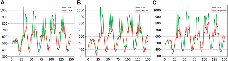
FIGURE 10. Comparison of the curves of four sampling points forecast using another reagional 7-day series by different methods. (A) LSTM; (B) Seq2Seq; (C) proposed.

FIGURE 11

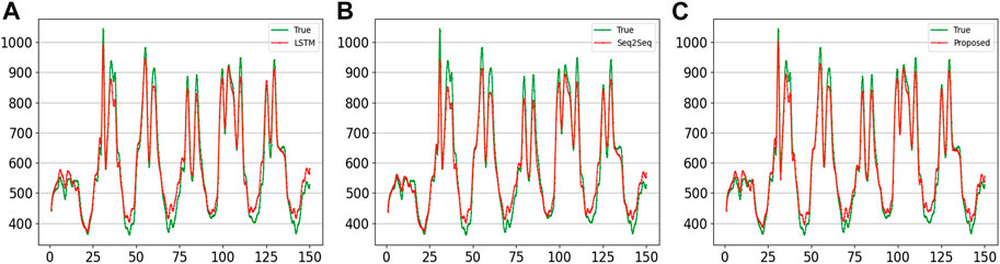
FIGURE 11. Comparison of the curves of next sampling points forecast using another reagional 7-day series by different methods. (A) LSTM; (B) Seq2Seq; (C) proposed.

Table 4 show the results of the indicators for the different methods for forecasting the load values for the next hour and 4 h. The same proposed method achieves the best values for all four indicators. This explains that at longer series lengths, the proposed method is better able to extract information from the historical data and to forecasting subsequent load values more accurately.

TABLE 4

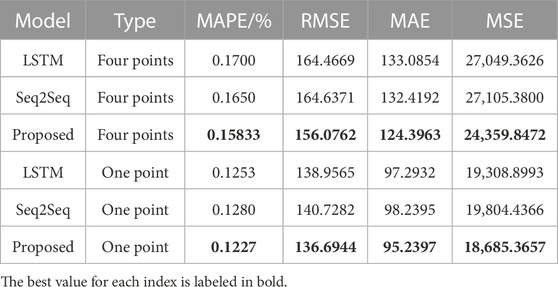
TABLE 4. Index values of four and one sampling points forecast using another reagional 7-day series by different methods.

5.3 Experimental summary

It can be seen through the above three experiments that the proposed method produced good forecasting results, and it also demonstrated remarkable competitiveness in terms of qualitative indicators. This can completely illustrate the use of multi-layer dilated LSTM as the Encoder structure, which can extract rich non-linear dependencies and multidimensional information from the original long time series. By emphasizing the information on the key historical time point and reducing the loss of historical information, the attention mechanism effectively improved the accuracy of load forecasting. It can be seen through experiments 1 and 2 that the longer the prediction time is concerned, the error will increase. Comparing experiments 1 and 3, the proposed method still produces more accurate predictions for the same length when the historical series is longer. Supplementary experiments show that when the length of the time series is reduced, the proposed model is still able to forecast short-term loads well but with a reduced accuracy compared to long series. This provides evidence that the proposed method can effectively handle the long series load forecasting problem.

6 Conclusion

Load forecasting is an important factor for the power system management. In this paper, we developed a load forecasting model based on multilayered dilated LSTM and attentional mechanism in the Seq2Seq framework. We first processed two actual experimental data, including feature selection, exception judgment, data filling, as well as other operations. Second, we normalized the data and divided them into various datasets in accordance with the training of neural networks. In this paper, a three-layer dilated LSTM model was established as an Encoder layer to extract the dependence from the original load series, and the context vectors focusing on key information are extracted through the attention layer. In the Decoder layer, LSTM was used for the decoding process, and a linear layer was used to output the forecast results. We then trained the proposed model and forecasted future values using the different datasets.

Our proposed model alleviated the limitation of information loss in long series information extraction of the conventional LSTM and excellently completed the task of using longer time series for more accurate load forecasting. On each of the two datasets in the experiment, we used historical series of different lengths to forecast future load values. The experimental results demonstrated that the proposed model not only outperforms the comparison methods in terms of load forecasting curves, but also shows stronger competitiveness in quantitative indicators. Therefore, the proposed model can effectively complete the tasks of information extraction from a long time series and prediction of future changes.

Data availability statement

The original contributions presented in the study are included in the article/Supplementary Material, further inquiries can be directed to the corresponding author.

Author contributions

YW: design, funding support, data and literature collection, preliminary analysis; CW: design, formal analysis, project administration; WJ: original draft, experiment implementation; QS: formal analysis, review; TZ: funding support, data and literature collection, preliminary analysis; QD: funding support, data and literature collection, preliminary analysis; XL: funding support, review. All authors contributed to the article and approved the submitted version.

Funding

This research was funded by the East Inner Mongolia Electric Power Co., Ltd., China, under Grant No. SGMDFWOOHSJS2200057, Jilin Provincial Science and Technology Department Project under Grant No. 20230601032FG, Jilin Province Science and Technology Development Plan Project—Innovation Platform (Base) and Talent Project under Grant No. 20230508037RC, and Strategic Research and Consulting Project of Chinese Academy of Engineering under Grant No. JL2022-16.

Conflict of interest

Authors YW, TZ, and QD were employed by Power Supply Service Supervision and Support Center of East Inner Mongolia Electric Power Co., Ltd.

The remaining authors declare that the research was conducted in the absence of any commercial or financial relationships that could be construed as a potential conflict of interest. The authors declare that this study received funding from East Inner Mongolia Electric Power Co., Ltd., China. The funder had the following involvement in the study: study design, data collection and experiment analysis.

Publisher’s note

All claims expressed in this article are solely those of the authors and do not necessarily represent those of their affiliated organizations, or those of the publisher, the editors and the reviewers. Any product that may be evaluated in this article, or claim that may be made by its manufacturer, is not guaranteed or endorsed by the publisher.

References

Aasim, , Singh, S. N., and Mohapatra, A (2021). Data driven day-ahead electrical load forecasting through repeated wavelet transform assisted svm model. Appl. Soft Comput.111, 107730. doi:10.1016/j.asoc.2021.107730

CrossRef Full Text | Google Scholar

Bahdanau, D., Cho, K., and Bengio, Y. (2014). Neural machine translation by jointly learning to align and translate. arXiv preprint arXiv:1409.0473.

Google Scholar

Bogomolov, A., Lepri, B., Larcher, R., Antonelli, F., Pianesi, F., and Pentland, A. (2016). Energy consumption prediction using people dynamics derived from cellular network data. EPJ Data Sci.5, 13–15. doi:10.1140/epjds/s13688-016-0075-3

CrossRef Full Text | Google Scholar

Chai, T., and Draxler, R. R. (2014). Root mean square error (rmse) or mean absolute error (mae)?–arguments against avoiding rmse in the literature. Geosci. Model. Dev.7, 1247–1250. doi:10.5194/gmd-7-1247-2014

CrossRef Full Text | Google Scholar

Chang, S., Zhang, Y., Han, W., Yu, M., Guo, X., Tan, W., et al. (2017). Dilated recurrent neural networks. Adv. neural Inf. Process. Syst.30.

Google Scholar

Ciechulski, T., and Osowski, S. (2021). High precision lstm model for short-time load forecasting in power systems. Energies14, 2983. doi:10.3390/en14112983

CrossRef Full Text | Google Scholar

Dai, Y., Zhou, Q., Leng, M., Yang, X., and Wang, Y. (2022). Improving the bi-lstm model with xgboost and attention mechanism: A combined approach for short-term power load prediction. Appl. Soft Comput.130, 109632. doi:10.1016/j.asoc.2022.109632

CrossRef Full Text | Google Scholar

Du, S., Li, T., Yang, Y., and Horng, S.-J. (2020). Multivariate time series forecasting via attention-based encoder–decoder framework. Neurocomputing388, 269–279. doi:10.1016/j.neucom.2019.12.118

CrossRef Full Text | Google Scholar

Gong, G., An, X., Mahato, N. K., Sun, S., Chen, S., and Wen, Y. (2019). Research on short-term load prediction based on seq2seq model. Energies12, 3199. doi:10.3390/en12163199

CrossRef Full Text | Google Scholar

Guo, Y., Li, Y., Qiao, X., Zhang, Z., Zhou, W., Mei, Y., et al. (2022). Bilstm multitask learning-based combined load forecasting considering the loads coupling relationship for multienergy system. IEEE Trans. Smart Grid13, 3481–3492. doi:10.1109/tsg.2022.3173964

CrossRef Full Text | Google Scholar

Hernandez, L., Baladron, C., Aguiar, J. M., Carro, B., Sanchez-Esguevillas, A. J., Lloret, J., et al. (2014). A survey on electric power demand forecasting: Future trends in smart grids, microgrids and smart buildings. IEEE Commun. Surv. Tutorials16, 1460–1495. doi:10.1109/surv.2014.032014.00094

CrossRef Full Text | Google Scholar

Hochreiter, S., and Schmidhuber, J. (1997). Long short-term memory. Neural Comput.9, 1735–1780. doi:10.1162/neco.1997.9.8.1735

PubMed Abstract | CrossRef Full Text | Google Scholar

Hussain, T., Min Ullah, F. U., Muhammad, K., Rho, S., Ullah, A., Hwang, E., et al. (2021). Smart and intelligent energy monitoring systems: A comprehensive literature survey and future research guidelines. Int. J. Energy Res.45, 3590–3614. doi:10.1002/er.6093

CrossRef Full Text | Google Scholar

Imani, M. (2021). Electrical load-temperature cnn for residential load forecasting. Energy227, 120480. doi:10.1016/j.energy.2021.120480

CrossRef Full Text | Google Scholar

Islam, M. J., Datta, R., and Iqbal, A. (2023). Actual rating calculation of the zoom cloud meetings app using user reviews on Google play store with sentiment annotation of bert and hybridization of rnn and lstm. Expert Syst. Appl.223, 119919. doi:10.1016/j.eswa.2023.119919

PubMed Abstract | CrossRef Full Text | Google Scholar

Jung, S., Moon, J., Park, S., and Hwang, E. (2021). An attention-based multilayer gru model for multistep-ahead short-term load forecasting. Sensors21, 1639. doi:10.3390/s21051639

PubMed Abstract | CrossRef Full Text | Google Scholar

Khan, A. R., Mahmood, A., Safdar, A., Khan, Z. A., and Khan, N. A. (2016). Load forecasting, dynamic pricing and dsm in smart grid: A review. Renew. Sustain. Energy Rev.54, 1311–1322. doi:10.1016/j.rser.2015.10.117

CrossRef Full Text | Google Scholar

Khan, S., Javaid, N., Chand, A., Khan, A. B. M., Rashid, F., and Afridi, I. U. (2019). “Electricity load forecasting for each day of week using deep cnn,” in Workshops of the international conference on advanced information networking and applications (Springer), 1107–1119.

CrossRef Full Text | Google Scholar

Khan, Z. A., Ullah, A., Haq, I. U., Hamdy, M., Maurod, G. M., Muhammad, K., et al. (2022). Efficient short-term electricity load forecasting for effective energy management. Sustain. Energy Technol. Assessments53, 102337. doi:10.1016/j.seta.2022.102337

CrossRef Full Text | Google Scholar

Kim, Y., Son, H.-g., and Kim, S. (2019). Short term electricity load forecasting for institutional buildings. Energy Rep.5, 1270–1280. doi:10.1016/j.egyr.2019.08.086

CrossRef Full Text | Google Scholar

Kwon, S. (2019). A cnn-assisted enhanced audio signal processing for speech emotion recognition. Sensors20, 183. doi:10.3390/s20010183

PubMed Abstract | CrossRef Full Text | Google Scholar

Li, K., Huang, W., Hu, G., and Li, J. (2023). Ultra-short term power load forecasting based on ceemdan-se and lstm neural network. Energy Build.279, 112666. doi:10.1016/j.enbuild.2022.112666

CrossRef Full Text | Google Scholar

Li, Y., Jia, Y., Li, L., Hao, J., and Zhang, X. (2020). Short term power load forecasting based on a stochastic forest algorithm. power Syst. Prot. control48, 117–124.

Google Scholar

Luong, M.-T., Pham, H., and Manning, C. D. (2015). Effective approaches to attention-based neural machine translation. arXiv preprint arXiv:1508.04025.

Google Scholar

Mahjoub, S., Chrifi-Alaoui, L., Marhic, B., and Delahoche, L. (2022). Predicting energy consumption using lstm, multi-layer gru and drop-gru neural networks. Sensors22, 4062. doi:10.3390/s22114062

PubMed Abstract | CrossRef Full Text | Google Scholar

Mohammed, N. A., and Al-Bazi, A. (2022). An adaptive backpropagation algorithm for long-term electricity load forecasting. Neural Comput. Appl.34, 477–491. doi:10.1007/s00521-021-06384-x

PubMed Abstract | CrossRef Full Text | Google Scholar

Moon, J., Park, S., Rho, S., and Hwang, E. (2019). A comparative analysis of artificial neural network architectures for building energy consumption forecasting. Int. J. Distributed Sens. Netw.15, 155014771987761. doi:10.1177/1550147719877616

CrossRef Full Text | Google Scholar

Patro, S., and Sahu, K. K. (2015). Normalization: A preprocessing stage. arXiv preprint arXiv:1503.06462.

Google Scholar

Paudel, S., Elmitri, M., Couturier, S., Nguyen, P. H., Kamphuis, R., Lacarrière, B., et al. (2017). A relevant data selection method for energy consumption prediction of low energy building based on support vector machine. Energy Build.138, 240–256. doi:10.1016/j.enbuild.2016.11.009

CrossRef Full Text | Google Scholar

Pavićević, M., and Popović, T. (2022). Forecasting day-ahead electricity metrics with artificial neural networks. Sensors22, 1051. doi:10.3390/s22031051

PubMed Abstract | CrossRef Full Text | Google Scholar

Peng, L., Lv, S.-X., Wang, L., and Wang, Z.-Y. (2021). Effective electricity load forecasting using enhanced double-reservoir echo state network. Eng. Appl. Artif. Intell.99, 104132. doi:10.1016/j.engappai.2020.104132

CrossRef Full Text | Google Scholar

Peng, L., Wang, L., Xia, D., and Gao, Q. (2022). Effective energy consumption forecasting using empirical wavelet transform and long short-term memory. Energy238, 121756. doi:10.1016/j.energy.2021.121756

CrossRef Full Text | Google Scholar

Qiao, W. (2018). Intelligent pre-estimation method study on short-period power load. Jiangsu Electr. J., 13–17.

Google Scholar

Rana, M., and Koprinska, I. (2016). Forecasting electricity load with advanced wavelet neural networks. Neurocomputing182, 118–132. doi:10.1016/j.neucom.2015.12.004

CrossRef Full Text | Google Scholar

Sehovac, L., and Grolinger, K. (2020). Deep learning for load forecasting: Sequence to sequence recurrent neural networks with attention. IEEE Access8, 36411–36426. doi:10.1109/access.2020.2975738

CrossRef Full Text | Google Scholar

Siami-Namini, S., Tavakoli, N., and Namin, A. S. (2019). A comparative analysis of forecasting financial time series using arima, lstm, and bilstm. arXiv preprint arXiv:1911.09512.

Google Scholar

Smyl, S. (2020). A hybrid method of exponential smoothing and recurrent neural networks for time series forecasting. Int. J. Forecast.36, 75–85. doi:10.1016/j.ijforecast.2019.03.017

CrossRef Full Text | Google Scholar

Smyl, S., Dudek, G., and Pełka, P. (2021). Es-Drnn: A hybrid exponential smoothing and dilated recurrent neural network model for short-term load forecasting. arXiv preprint arXiv:2112.02663

Google Scholar

Staudemeyer, R. C., and Morris, E. R. (2019). Understanding lstm–a tutorial into long short-term memory recurrent neural networks. arXiv preprint arXiv:1909.09586.

Google Scholar

Su, X., Liu, T., Cao, H., Jiao, H., Yu, Y., He, C., et al. (2017). A multiple distributed bp neural networks approach for short-term load forecasting based on hadoop framework. Proc. CSEE37, 4966–4973.

Google Scholar

Sutskever, I., Vinyals, O., and Le, Q. V. (2014). Sequence to sequence learning with neural networks. Adv. neural Inf. Process. Syst.27.

Google Scholar

Wang, Y., Sun, S., Chen, X., Zeng, X., Kong, Y., Chen, J., et al. (2021a). Short-term load forecasting of industrial customers based on svmd and xgboost. Int. J. Electr. Power and Energy Syst.129, 106830. doi:10.1016/j.ijepes.2021.106830

CrossRef Full Text | Google Scholar

Wang, Y., Zhong, M., Han, J., Hu, H., and Yan, Q. (2021b). “Load forecasting method of integrated energy system based on cnn-bilstm with attention mechanism,” in 2021 3rd international conference on Smart power and internet energy systems (SPIES) (IEEE), 409–413.

CrossRef Full Text | Google Scholar

Wei, L., and Zhen-gang, Z. (2009). “Based on time sequence of arima model in the application of short-term electricity load forecasting,” in 2009 international conference on research challenges in computer science (IEEE), 11–14.

CrossRef Full Text | Google Scholar

Wu, K., Wu, J., Feng, L., Yang, B., Liang, R., Yang, S., et al. (2021). An attention-based cnn-lstm-bilstm model for short-term electric load forecasting in integrated energy system. Int. Trans. Electr. Energy Syst.31, e12637. doi:10.1002/2050-7038.12637

CrossRef Full Text | Google Scholar

Yang, B., Yin, K., Lacasse, S., and Liu, Z. (2019). Time series analysis and long short-term memory neural network to predict landslide displacement. Landslides16, 677–694. doi:10.1007/s10346-018-01127-x

CrossRef Full Text | Google Scholar

Yang, Y. (2022). Application of lstm neural network technology embedded in English intelligent translation. Comput. Intell. Neurosci.2022, 1–9. doi:10.1155/2022/1085577

CrossRef Full Text | Google Scholar