Identify incipient faults through similarity comparison with waveform split-recognition framework

1 Introduction

Detection of faults is a crucial problem for distribution networks. The economic losses caused by power failures can be avoided by detecting the faults immediately. In recent years, with the development of fault detection equipment, the rate of fault occurrence in distribution networks is decreasing. However, it has been observed that 10 to 15 percent of cable faults are preceded by incipient faults Kasztenny et al. (Cui et al., 2008); Kim et al. (2013). Incipient faults in underground cables fundamentally result from moisture, watering trees, or tracking (or electrical treeing) Kulkarni et al. (Kulkarni et al., 2010). They are self-clearing faults accompanied by electric arcs. Therefore, incipient faults are usually detected as a faulty phenomenon with a comparatively lower fault current and shorter fault time about 1/4 cycle to 4 cycles. So, these current changes are not detectable by common protection schemes Jannati et al. (2019). Over the past decades, extensive research has been conducted on incipient faults detection Stringer and Kojovic (2001); Moghe et al. (Moghe et al., 2009); Kulkarni et al. (2014). However, detection of incipient faults is still a challenging task.

Methods to detect incipient faults are mainly mathematical models which extract features from the waveform and then make decisions based on these features. Features can be extracted from the time domain and frequency domain. Sarlak and Shahrtash. (2013) is implemented in the time domain by utilizing waveform data collected from power quality monitors and relays to estimate the distance to the fault in terms of the line impedance. Kim and Bialek (Kim and Bialek, 2011) proposes a new time domain approach for locating the sub-cycle incipient failure. Sidhu and Xu (2010) is based on superimposing fault current and negative sequence current in the time domain. After the decomposition by wavelet analysis, two detection rules are proposed according to different frequency bands, and three classification rules are accomplished by Root Mean Square (RMS) value and maximum and minimum value. In the frequency domain, Zhang et al. (2017) adopts Fast Fourier Transform (FFT) to analyze the fault point voltage and calculate the voltage total harmonic distortion (THD). Radojevic et al. (2013) followed the frequency domain harmonic analysis and detailed frequency domain fault equations are built to estimate fault resistance for arcing fault detection. Inter harmonics have been used for fault detection Tao Cui et al. (Kasztenny et al., 2008). A large number of approaches in the literature are based on wavelet technique Ghaderi et al. (2015); Zhou et al. (Zhou et al., 2015); Elkalashy et al. (2008); Xiong et al. (2020); Mousavi and Butler-Purry (2010); Sedighi et al. (2005). The wavelet analysis can analyze the physical situations where signals contain discontinuities, abrupt changes, and sharp spikes, and then separate different frequency components into different frequency bands. The wavelet-based high-impedance fault (HIF) detector proposed by Michalik et al. utilizes the phase displacement between wavelet coefficients Michalik et al. (2006). An arcing fault is claimed when the measured voltage and current signals match the arcing fault model better than the non-arcing disturbance model Zhang et al. (2016). Most of the above methods to extract electric features ignore some higher harmonics, which will result in the loss of information transmitted by waveform. The better way is to retain all information through image recognition Song and Chang (2009); Simonyan and Zisserman (2015); Li (2015).

Considering the random changes in network structure, line parameters, load, and noise, these methods have difficulty identifying incipient faults. A good way to handle randomness and uncertainty associated with incipient faults is data-driven methods Guo et al. (2018); Liu and Huang (2018). Following the development of information science and hardware devices, using big data to model and analyze complex problems has become a worldwide trend. Compared to the traditional model-based methods, data-driven methods can extract features and knowledge from an unknown system without the help of domain experts. However, traditional data-driven methods require a large amount of historical data to conduct data mining and eigenvalue analysis, but incipient faults obviously do not have such conditions. Xu. (2018) provides a single-phase incipient fault in underground cable originating from an incipient failure of an XLPE cable. It can be seen from Figure 1 that the voltage of the fault phase does not increase significantly, and the current of the fault phase only lasts for a one-half cycle. Incipient faults do not trigger protective devices due to the short duration and low fault current magnitude. So, the fault has great difficulty detecting the equipment. Therefore, maintenance personnel is usually not aware of their occurrence. This makes it difficult to collect incipient faults data, making incipient faults a small sample problem.

FIGURE 1

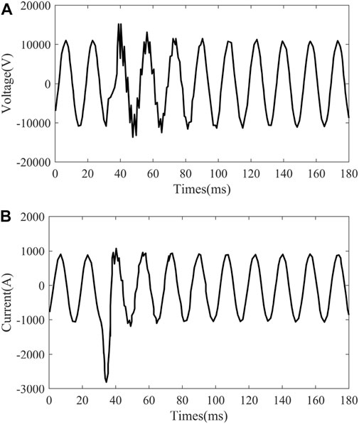
FIGURE 1. Waveform from a single-phase incipient fault in underground cable. (A) Voltage wave form of fault phase, (B) current wave form of fault phase.

One-shot learning can discover much information about a category from one or several images. Neural networks are very good at extracting features from high-dimensional data. However, this advantage of neural networks becomes a major obstacle to their small sample learning. It is easy for humans to learn a class of features from a single sample because we have been observing and learning from similar objects all our lives. It is not fair to compare a randomly initialized neural network with a human network that spends a lifetime identifying objects and symbols, because the randomly initialized neural network lacks a prior knowledge for the data mapping structure. Thus, we adopt knowledge transfer methods from other tasks. Therefore, this paper proposes an incipient fault detection method based on one-shot learning. The three contributions of this paper are summarized as follows:

•A WSRF is proposed to identify the incipient faults in distribution networks. Split the waveform into several segments according to cycles and make a decision that the possibility of incipient faults is calculated by the similarity of each segment.

•We design SCN to compare the similarity of two waveforms by combining two CNNs and sharing weights. Calculate the difference between two inputs through a non-linear function that can deal with the similarity in the range of 0 to 1.

•Disassembled filters with initial weights is devised to extract features that represent the deformation of a waveform. The initial weights are shown to be effective if acquired from the training of classical image datasets.

The outline of the paper is presented as follows: Section 2 gives a description of WSRF to identify the incipient faults. Section 3 brings an introduction to SCN to calculate the similarity of the waveform in the power grid. Based on the proposed method, Section 4 suggests an idea that uses disassembled filters with initial weights to extract feature maps. Section 5 demonstrates the numerical results of WSRF and compares it with other classifiers. The conclusion is in Section 6.

2 Waveform split-recognition framework

Waveform split-recognition is inspired by the human perception of the waveform. When observing a waveform, humans tend to divide it into several segments. Features of segments are both perceived by humans to help them distinguish different waveforms and even understand the electrical processes behind them. Due to the waveform of incipient faults lasting between a quarter and four cycles, it is impossible to set the length of a unit of time. A comparison of waveforms is needed to ensure that the two images of each waveform are conducted in the same period. Otherwise, the comparison has no effect on incipient faults identification. Therefore, WSRF is proposed to decompose waveform into several segments, as shown in Figure 2. General shape w₁, w₂, w₃, w₄, w₅, …, w_n are the components of the waveform, which are called primitives in the WSRF. Instead of being described directly, waveform described by primitives can be much easier and has a better performance Lake. (2014).

FIGURE 2

FIGURE 2. An illustration of WSRF: the current of a faulted phase in a cable incipient fault is split into several segments.

The type of abnormal events in the distribution system depends on the occurrence of the fault, and the type of fault can be seen from the waveform. The waveform of different event types is different. In this paper, based on WSRF, the fault phase waveform of event ψ is decomposed by several periodic waveforms ψ₁, ψ₂, …, ψ_n. So, the possibility of failure is obtained by comparing the similarity of these periodic waveforms. Abnormal events of the same type may have different behaviors in voltage and current waveform, which are written as event cases ψ¹, ψ², …, ψ^k. Compare an unknown event to each case of a certain event and identify the event by the case which is the highest similarity. The probability of an unknown event θ to be a certain event ψ can be written as:

$P\left(\theta |\psi \right)=\max \left(\prod _{i=1}^{n}P\left({\theta }_i|{\psi }_i^1\right),\prod _{i=1}^{n}P\left({\theta }_i|{\psi }_i^2\right),\dots ,\prod _{i=1}^{n}P\left({\theta }_i|{\psi }_i^k\right)\right),(1)$

where n is the number of cycles recorded for an event, k is the number of cases for event ψ. θ_i is the ith periodic waveform in an unknown event case θ, and ${\psi }_i^1$ is the ith periodic waveform of case 1 in event ψ.

Here the order of phases in an event is adjusted. It should be noted that the fault phase does not affect the event type. For example, an incipient fault happening in Phase A and another happening in Phase B with the same root cause are considered the same type. Incipient faults severity is closely related to the current pulse magnitude. So, the cycle order starts from the cycle with the highest current pulse magnitude.

3 Similarity Comparison Network

SCN can acquire feature maps that enable the model to generalize successfully from a few examples. The detailed architecture is shown in Figure 3. It is a conjoined neural network, which is reflected by sharing weights to measure the similarity of two inputs. Two inputs (w₁ and w₂) are fed into neural networks (Network₁ and Network₂). These two neural networks map the inputs to the new space respectively, forming the representation of the inputs in the new space. Through the calculation of distance in high-dimensional space, the similarity between the two inputs is calculated by a non-linear function.

FIGURE 3

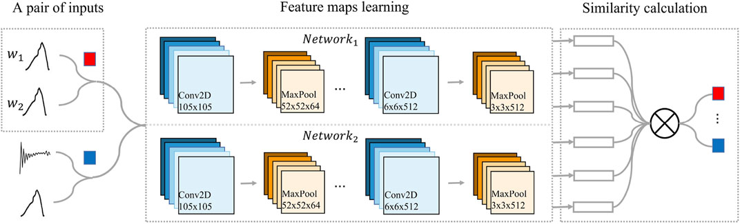
FIGURE 3. Architecture of SCN: Convolutional Neural Network architecture followed by non-linear layers to convert embeddings into the probabilistic output of possible categories.

3.1 Structure of model

This model is structurally divided into two steps: feature maps learning and similarity calculation. The waveform of the power grid is processed by WSRF into several images, and the size of each image is 105 × 105. The feature maps learning section has two convolutional neural networks each with L layers. One layer has N_l units and h_l hidden vectors. Each convolution layer uses a single channel with filters of different sizes and a fixed step size of 1 to capture the unapparent distortion of the waveform more completely. At the same time, the number of convolution filters is specified as a multiple of 16 to optimize performance in extracting feature maps from the waveform. The network applies Rectified Linear Unit (ReLU) activation function to the output feature map of the waveform. For pooling mode, max-pooling is selected. Considering the specification of the waveform and the number of convolution layers, max-pooling with a step size of 2 is adopted. Therefore, the kth feature map in each convolutional pooling layer is in the following form:

$a_l^{\left(k\right)}=\max -pool\left(\max \left(0,W_l^{\left(k\right)}\otimes h_l+b_l\right),2\right),(2)$

where W_l is the 3-dimensional tensor representing the feature maps for layer l. We take ⊗ to be the convolutional operation corresponding to those output units which are the result of the complete overlap between each convolutional filter and the input feature maps. b_l is the correction factor in layer l.

In a similar calculation step, the units from the final convolutional-pooling layer are flattened into a single vector. This convolutional layer is followed by a fully connected layer. In the fully connected layer, the activation function is ReLU which chooses feature maps for the following similarity comparison. One more layer computing the induced distance metric between siamese twins, which is given to a non-linear function output unit. More precisely, the prediction vector is given as follows:

$S\left(w_1,w_2\right)=\frac{1}{1+\exp \left(-{\sum }_{i=1}^n{\beta }_i\left|f_1^i-f_2^i\right|\right)},(3)$

where β_i is the additional parameter learned when the model measures the distance during training. This defines a final fully connected layer for the network which joins the two siamese twins. $f_1^i$ represents the ith feature map from Network₁, $f_2^i$ represents the ith feature map from Network₂.

3.2 Loss function

Since there are two cases of labels input by SCN, the loss function should also be discussed in different situations. The loss function adopted in this model is inspired by contrastive loss, It is shown in the following equation.

$L\left(w_1,w_2\right)=\left\{\begin{array}{cc}{D_w}^2\hfill & y=0,\hfill \\ {\max \left(0,D_w-m\right)}^2\hfill & y=1,\hfill \end{array}\right.(4)$

where D_w is the distance between two waveforms in high-dimensional space. y = 1 means that the two waveforms are from the same incipient fault, and y = 0 is the opposite. For the same waveform, we want its loss function to be as small as possible, but it cannot be completely zero for the waveform in a power grid. We give a threshold value of m. For different input pairs, the larger the difference, the more irrelevant are the two inputs.

3.3 Optimization criteria

The optimization in this paper is based on the back-propagation algorithm. Since Network₁ and Network₂ share weight, the gradient is additive. We fix the learning rate, momentum, and regularization weight, so the optimization criterion of the Tth epoch is as follows:

$\begin{array}{c}\hfill W_{k_j}^{\left(T\right)}\left(w_1^{\left(i\right)},w_2^{\left(i\right)}\right)=W_{k_j}^{\left(T\right)}+△W_{k_j}^{\left(T\right)}\left(w_1^{\left(i\right)},w_2^{\left(i\right)}\right)+2{\lambda }_j|W_{k_j}|,\\ \hfill △W_{k_j}^{\left(T\right)}\left(X_1^{\left(i\right)},X_2^{\left(i\right)}\right)=-{\eta }_j▽W_{k_j}^{\left(T\right)}+{\mu }_j△W_{k_j}^{\left(T-1\right)},\end{array}(5)$

where $▽W_{k_j}$ is the partial derivative with respect to the weight between the jth neuron in one layer and the kth neuron in the successive layer.

3.4 Learning schedule

We allow each layer to have different learning rates, but the attenuation of learning rates is consistent throughout the network. We find that by annealing learning, the network can converge to the local minimum more easily without getting stuck in the error surface. Our momentum in each layer starts from 0.9 and increases linearly in each period until it reaches the value μ_j. We train each network for a maximum of 100 epochs and set the action of delaying the learning rates uniformly across the network by 50 percent per epoch when there are 5 epochs and the performance of the past model still does not improve, that is ${\eta }_j^{(T)}=0.5{\eta }_j^{(T-1)}$. If validation errors continue to decrease throughout the learning plan, we save the final state of the model generated by this process.

4 Disassembled filters with initial weights

4.1 Disassembled filters

The selection of filters has an important impact on feature extraction which is the basis of identification. The filter with a large specification is selected at the beginning due to the sparsity of the waveform pixel matrix. However, large filters may lead to an excessive parameter calculation and take up a lot of time and resources. At the same time, according to Simonyan and Zisserman. (2015), the depth of the neural network is directly related to the performance of the network: the deeper the depth, the better the network performance. Based on the above two points, we propose disassembled filters to extract features of the waveform as shown in Figure 4. It not only avoids the use of large filters but also increases the depth of the convolution network. In addition, the filter also reduces the number of weights that need to be calculated iteratively and reduces the computational burden. The convolution formula is as follows:

$E_o=E_i\otimes F_d^1\otimes \cdots \otimes F_d^k,(6)$

where ⊗ represents convolutional operation. $E_o=\left[\begin{array}{cccc}\hfill O_{11}\hfill & \hfill O_{12}\hfill & \hfill \cdots \hfill & \hfill O_{1n}\hfill \\ \hfill O_{21}\hfill & \hfill O_{22}\hfill & \hfill \cdots \hfill & \hfill O_{2n}\hfill \\ \hfill ⋮\hfill & \hfill ⋮\hfill & \hfill \ddots \hfill & \hfill ⋮\hfill \\ \hfill O_{m1}\hfill & \hfill O_{m2}\hfill & \hfill \cdots \hfill & \hfill O_{mn}\hfill \end{array}\right]$ and $E_i=\left[\begin{array}{cccc}\hfill I_{11}\hfill & \hfill I_{12}\hfill & \hfill \cdots \hfill & \hfill I_{1n}\hfill \\ \hfill I_{21}\hfill & \hfill I_{22}\hfill & \hfill \cdots \hfill & \hfill I_{2n}\hfill \\ \hfill ⋮\hfill & \hfill ⋮\hfill & \hfill \ddots \hfill & \hfill ⋮\hfill \\ \hfill I_{m1}\hfill & \hfill I_{m2}\hfill & \hfill \cdots \hfill & \hfill I_{mn}\hfill \end{array}\right]$ are the output matrix and input matrix of the convolution layer respectively. While $F_d^1=\left[\begin{array}{cccc}\hfill D_{11}^{(1)}\hfill & \hfill D_{12}^{(1)}\hfill & \hfill \cdots \hfill & \hfill D_{1q}^{(1)}\hfill \\ \hfill D_{21}^{(1)}\hfill & \hfill D_{22}^{(1)}\hfill & \hfill \cdots \hfill & \hfill D_{2q}^{(1)}\hfill \\ \hfill ⋮\hfill & \hfill ⋮\hfill & \hfill \ddots \hfill & \hfill ⋮\hfill \\ \hfill D_{p1}^{(1)}\hfill & \hfill D_{p2}^{(1)}\hfill & \hfill \cdots \hfill & \hfill D_{pq}^{(1)}\hfill \end{array}\right]$ and $F_d^k=\left[\begin{array}{cccc}\hfill D_{11}^{(k)}\hfill & \hfill D_{12}^{(k)}\hfill & \hfill \cdots \hfill & \hfill D_{1q}^{(k)}\hfill \\ \hfill D_{21}^{(k)}\hfill & \hfill D_{22}^{(k)}\hfill & \hfill \cdots \hfill & \hfill D_{2q}^{(k)}\hfill \\ \hfill ⋮\hfill & \hfill ⋮\hfill & \hfill \ddots \hfill & \hfill ⋮\hfill \\ \hfill D_{p1}^{(k)}\hfill & \hfill D_{p2}^{(k)}\hfill & \hfill \cdots \hfill & \hfill D_{pq}^{(k)}\hfill \end{array}\right]$ are the disassembled filters.

FIGURE 4

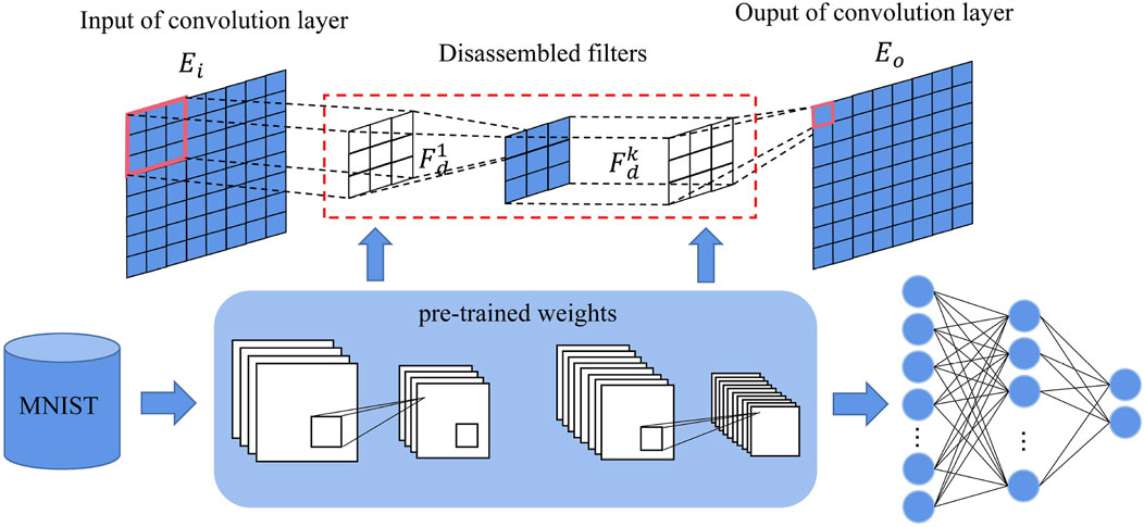
FIGURE 4. Schematic diagram of disassembled filters with initial weights: pre-trained weights from MNIST are used as the initial weights in disassembled filters.

4.2 Weight initialization

The incipient fault detection of distribution networks usually cannot obtain a large amount of relevant data, and the random initialization parameters may lead to over-fitting and unsatisfactory results. Initializing the neural network with appropriate weights has a positive effect on the training and optimization of the network. The tasks of each layer of the neural network for image recognition are different. The low layers extract features of the image (such as edge detection and color detection), which are general for many tasks and the high layers extract features related to specific categories Zeiler and Fergus. (2013). Therefore, we use fine-tuning method to initialize the disassembled filter. As shown in Figure 4: only weights of low layers are obtained by MNIST, and that of the high layers is initialized randomly.

MNIST and fault data have some same characteristics, such as white background, black line, and sparse pixel matrix. Simulation data and fault data are all waveform data and have a lot of same characteristics. Therefore, We use three initialization methods: initialized by MNIST, initialized by simulation data, and random initialization. The results of three methods are presented in Figure 5. The Accuracy of random initialization is lower than the other two. Although the simulation data initialization has a good start, the final result is not as good as MNIST initialization. Therefore, it is a good choice to use MNIST to initialize the weights. Learning weights from a dataset with different data distribution by fine-tuning like this has been evidenced by Yosinski et al. (2014) and has been applied in medical image recognition Morid et al. (2021).

FIGURE 5

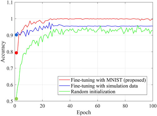
FIGURE 5. Accuracy of SCN with different initial weights.

5 Numerical results

After discussing the classification of incipient faults, this section proposes some metrics to evaluate the methods. This section demonstrates the performance of disassembled filters with initial weights in SCN by using filed data. After comparing WSRF with other methods, a discussion of WSRF is provided.

5.1 Data source

According to the filed data collected from Xu. (2018) and Mohsenian-Rad. (2022), we have a deep understanding of various grid faults. Through waveform analysis and field identification, three categories of abnormal events are found: incipient faults, permanent faults, and transient disturbances. At the same time, we also find many cases of the same fault type under different circumstances. Take incipient faults as an example. The incipient faults occurring on different equipment can be different cases of incipient faults, such as cable incipient faults, overhead line incipient faults, switch incipient faults, etc. Furthermore, there are two types of incipient faults in the same equipment according to the duration of the arc: sub-cycle and multi-cycle. The sub-cycle incipient fault and multi-cycle incipient fault that occurred on the cable are shown in Figure 6.

FIGURE 6

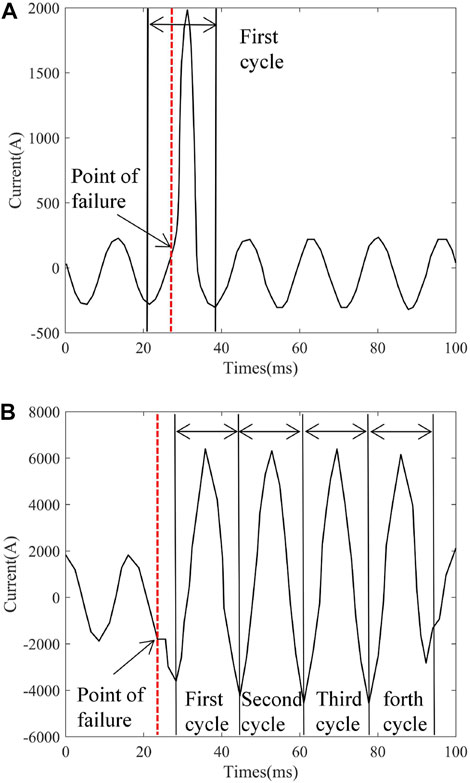
FIGURE 6. The current waveform of fault phase in sub-cycle incipient fault and multi-cycle incipient fault from cable. (A) Sub-cycle incipient fault, (B) multi-cycle incipient fault.

5.2 Evaluation metrics

To evaluate performance and understand machine learning models, we propose a series of evaluation indicators. Accuracy is introduced as a measure of model performance. A good performance is related to high Accuracy. Accuracy is an excellent measure only when we have symmetric datasets where false positives and false negatives are almost the same. Therefore, the F1 is usually more useful than Accuracy, especially if we have an uneven class distribution. The F1 is the weighted average of precision and recall. Therefore, this score takes both false positives and false negatives into account. So, to summarize, the idea is that: Accuracy works best if false positives and false negatives have similar costs. If the cost of false positives and false negatives is very different, it’s better to look at the F1. The formula of Accuracy, Precision, Recall, and F1 are given as:

$Accuracy=\frac{t_p+t_n}{t_p+t_n+f_p+f_n},(7)$

$Precision=\frac{t_p}{t_p+f_p},(8)$

$Recall=\frac{t_p}{t_p+f_n},(9)$

$F1=\frac{2*Precision*Recall}{Precision+Recall},(10)$

where t_p: true positive (the predicted type and actual type are all 1), f_p: false positive (the predicted type is 0, but the actual type is 1), t_n: true negative (the predicted type and actual type are all 0), f_n: false negative (the predicted type is not 0, while the actual type is 0).

5.3 Comparison between SCN and convolutional neural network

In this subsection, we focus on evaluating the performance of disassembled filters with initial weights in SCN. To improve the applicability of this model, we adopt images from incipient faults in four types of electrical equipment: cable, overhead line, transformer, and switch. 20 sub-types are defined and 40 cases are generated for each sub-type under different external environmental conditions. The event type distribution is presented in Table 1. Specifically, the datasets contain 800 abnormal data, of which 560 data are selected as the training set. Two images are randomly selected as the input of SCN, and the result is compared with the input label. The results of fault image similarity comparison between CNN, SCN, and SCN with initial weights are shown in Figure 7.

TABLE 1

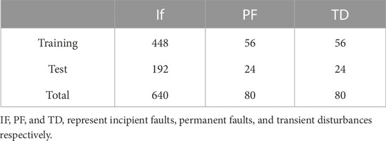
TABLE 1. Event number distribution of each dataset.

FIGURE 7

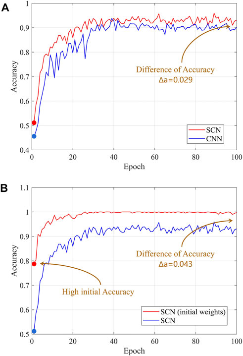
FIGURE 7. Training process of CNN, SCN, and SCN with initial weights. (A) Comparison between CNN and SCN, (B) comparison between SCN and SCN with initial weights.

From Figure 7 we can find that: due to loss of initial weights, their initial Accuracy is not high. With continuous iterative optimization, CNN with normal filters obtains an Accuracy of 0.902. SCN with disassembled filters can achieve higher Accuracy than CNN. The initial Accuracy of SCN is only 0.511, but the performance of optimization is good. SCN finally achieves an Accuracy of 0.931 after optimization iterations. Figure 7 shows a comparison between SCN and SCN with initial weights. SCN with initial weights has a relatively higher initial Accuracy of 0.790, and an Accuracy of 0.998 is obtained. Through analysis, SCN with initial weights has better results in Accuracy than CNN.

5.4 Performance analysis of SCN

5.4.1 Identification of incipient faults in field data

This subsection shows the practicability of SCN in different filed data from Xu. (2018); Mohsenian-Rad. (2022). First, we discuss the performance of SCN in data from Xu. (2018). Performance of SCN in different electrical equipment is shown in Figure 8. Each device has 648 inputs (324 same inputs and 324 different inputs). From Figure 8 we can see that when the input pairs are the same among the output of cable waveform, all results are between 0.5 and 0.7. Of the results, 283 of the overhead line are between 0.6 and 0.8, while 251 of the result of the transformer is between 0.5 and 0.6. 263 results of the switch are more than 0.5, while 61 results are less than 0.5. According to the above information, when the input pairs are the same, the waveform comparison results of the four electrical equipment have a concentrated distribution between 0.5 and 0.7. The results of different input pairs are shown in Figure 8. Of the results, the 280 results of the cable are less than 0.1. Similarly, 280 results of the overhead line are between 0 and 0.1, and 278 results of the transformer are less than 0.1. 259 results of the switch are less than 0.1. The remaining results are scattered between 0.1 and 1. It can be seen that when the input pairs are different, the results of SCN are concentrated between 0 and 0.1. In order to show the performance of SCN more intuitively, set the threshold to 0.5. The Accuracy, Precision, Recall, and F1 of SCN on the four types of equipment are presented in Table 2. We can see that the Accuracy of cable, overhead line, and transformer waveform images are more than 0.94, and F1 of them are more than 0.94. Only the Accuracy on the switch is relatively low, but it is also as high as 0.85, and F1 is 0.845. In this way, the SCN model has a very good classification performance on waveform images.

FIGURE 8

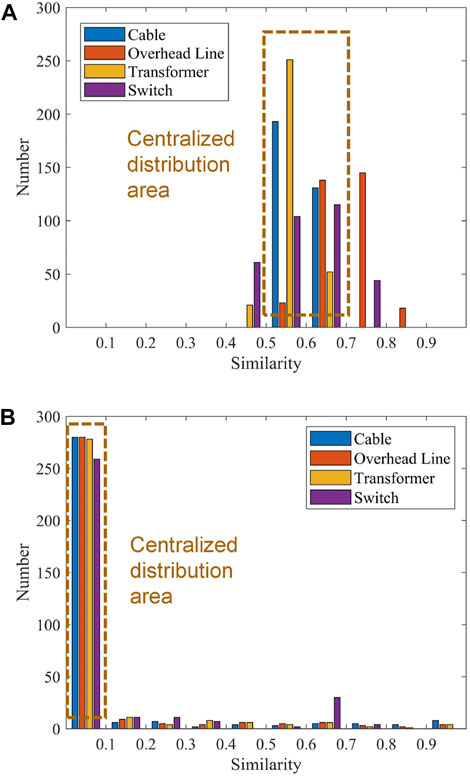
FIGURE 8. Performance of SCN in different electrical equipment. (A) Input image pair is the same, (B) input image pair is different.

TABLE 2

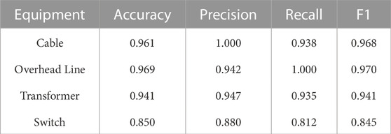
TABLE 2. Identification results of SCN from Xu. (2018).

Besides, we use the data from Mohsenian-Rad. (2022) to prove the practicability of this method. 1,000 validation results (500 negative samples and 500 positive samples) are presented in Table 3. Accuracy, Precision, Recall, and F1 achieve good results, with the smallest pPrecision of 0.829. The most important evaluation index F1 also reached 0.841. Therefore, we can draw the conclusion that this method is practical for incipient faults identification in distribution networks from the real world.

TABLE 3

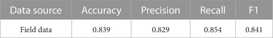
TABLE 3. Identification results of SCN from Mohsenian-Rad. (2022).

5.4.2 Factors affecting identification

This subsection takes the cable line as an example to analyze the influence of various factors on the incipient faults identification of SCN. We refer to one of our authors Cui et al. (2019) to establish the benchmark system which can be found in Figure 9. The system configuration under different distributed energy resource (DER) technologies is presented in Table 4. The wind farm is Type 4 and rated at 575 V, 6.6 MVA. According to IEEE Standard 1,547, the wind farm adopts constant power control with LVRT capability. The maximum fault current is limited to 1.5 pu.

FIGURE 9

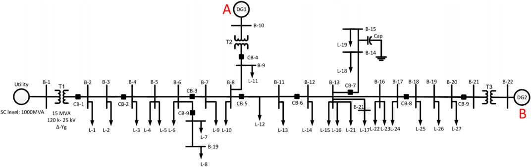
FIGURE 9. Single line diagram of distribution feeder.

TABLE 4

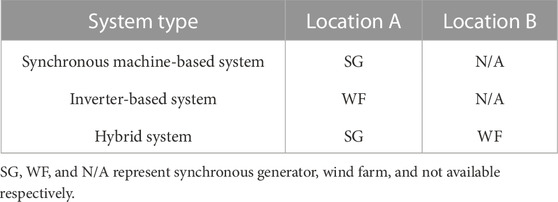
TABLE 4. System configuration under different DER technologies.

We evaluate the performance of SCN in cable lines in terms of different fault locations, fault occurrence time, and fault impedance. The performance of SCN is presented in Table 5:

• Fault location: The three fault locations are shown in Figure 9. Location 1 near bus B-3, location 2 near bus B-11, and location 3 near bus B-19. From Table 5, we find that SCN can achieve good results in three locations. Accuracy and F1 at location 1 are 0.945 and 0.893 respectively. Although the result obtained at location 2 is not as good as that at location 1, this does not mean that the performance of SCN is affected, because the Accuracy and F1 at location 3 also achieve a high score, both of which greater than 0.9.

• Fault occurrence time: The step module is used to control the fault occurrence time to simulate many incipient faults in cable lines occurring at different times. We trigger incipient faults at the beginning of simulation, 0.2 s after the beginning of simulation and 0.4 s after the beginning of simulation. From Table 5, we find that SCN can achieve very good results in three occurrence times. The Accuracy of the three occurrence times is between 0.825 and 0.858, and F1 is between 0.834 and 0.868. The time of fault occurrence has a little direct relationship with the Accuracy of the identification.

• Fault impedance: By adjusting the resistance value of incipient faults in cable line, the influence of resistance change on incipient faults identification is analyzed in Table 5. We find that changing the resistance affects the recognition of SCN. When the resistance value is 20, the Accuracy and F1 are as high as 0.882 and 0.885 respectively. However, when the resistance value is 10, the Accuracy and F1 are 0.722 and 0.676. This shows that the change of resistance has an impact on the Accuracy of SCN identification.

TABLE 5

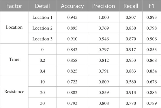
TABLE 5. Simulation results of cable incipient faults identification.

According to the previous analysis, for incipient faults of cable, the location and time of fault occurrence have no great impact on the Accuracy of identification. Because changing the location of the fault will not change the fault waveform. The same is true for the time of failure. However, changing the fault resistance value will affect the waveform change and will have some negative effects on the Accuracy.

5.4.3 Identification of arc faults

An arc fault is one of the incipient faults most likely to occur in the distribution network. Generally, the fault arc contains many complex characteristics with non-linear changes, which will affect the performance of incipient faults identification. It is necessary to analyze the influence of fault arc on the discussed algorithm. So, we refer to one of our authors Cui et al. (2019) to model the fault arc. As shown in Figure 10: This model connects one phase of the power line to the ground. Two variable resistors are both changing randomly and model the dynamic arcing resistance. Two sets of diodes and DC sources are connected in an anti-parallel configuration. The two DC sources are randomly varying as well, which models the asymmetric nature of arc faults.

FIGURE 10

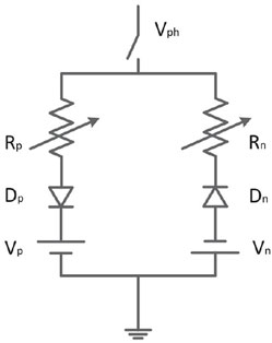
FIGURE 10. Arc faults model: two anti-parallel dc-source model. The positive half cycle of arc faults current is achieved when V_ph > V_p, while the negative half cycle is when V_ph < V_n. When V_n < V_ph < V_p, the current equals zero, which represents the period of arc extinction.

Similar to section 5.4.2, we replace the cable faults with arc faults and evaluate the performance of SCN in arc faults in terms of different fault locations, fault occurrence time, and fault impedance. The performance of SCN is presented in Table 6:

• Fault Location: Three fault locations are shown in Figure 9. From Table 6, we find that Accuracy and F1 at location 1 are 0.800 and 0.827 respectively. Although the high values of 0.908 and 0.915 were obtained at location 2, unsatisfactory results of 0.735 and 0.683 were obtained at location 3. The above shows that the location of the arc faults has an impact on the Accuracy of recognition because the uncertainty and non-linearity of the fault arc make it challenging to identify through images.

• Fault occurrence time: The step module is also used to control the fault occurrence time to simulate the arc faults at different times. We trigger arc faults at the beginning of simulation, 0.2 s after the beginning of simulation and 0.4 s after the beginning of simulation. From Table 6, we find that SCN can achieve very good results in three occurrence times. The Accuracy of the three occurrence times is 0.886, 0.893, and 0.903. F1 is 0.890, 0.898 and 0.909. Therefore, there is almost no direct relationship between the time of arc faults occurrence and the Accuracy of identification.

• Fault Impedance: By adjusting R_P and R_n to change the resistance value of arc faults, the influence of resistance change on arc faults identification is analyzed. From Table 6, the Accuracy of arc faults in different resistance is 0.875, 0.908, and 0.875. F1 also achieved a higher value of 0.879, 0.915, and 0.884. Therefore, we find that the Accuracy of the arc faults is not related to the resistance value. SCN achieves good results in arc faults identification.

TABLE 6

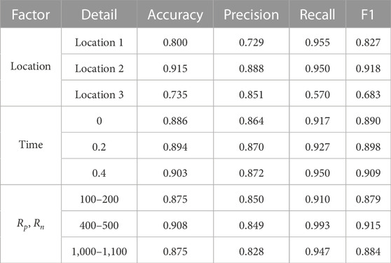
TABLE 6. Simulation results of arc faults identification.

According to the previous analysis, for arc faults, the time of fault occurrence and fault resistance value have no great impact on the Accuracy of identification. Changing the time of fault occurrence will not change the fault waveform. Due to the non-linear characteristics of arc faults, changing the fault location will change the waveform to a certain extent, thus affecting the Accuracy of identification.

5.5 Compare WSRF with other methods

Presently, the popular methods in the field of image recognition are SVM, CNN, and BP. The characteristics of Song and Chang. (2009), Simonyan and Zisserman. (2015), Li. (2015), and WSRF in incipient fault recognition are shown in Table 7. Song and Chang. (2009) is a binary classification model, which maps the linear inseparable data in the input space to the high-dimensional feature space and then obtains the separation hyperplane with the correct division of the datasets and the largest geometric interval. Simonyan and Zisserman. (2015) is a feedforward neural network, which is composed of neurons with learnable weights and bias constants. WSRF and Simonyan and Zisserman. (2015) use the same method to extract waveform image feature maps. Li. (2015) is a multi-layer feedforward perceptron network, which is trained by back-propagation to minimize the sum of squares of the network errors. By constantly adjusting weights and thresholds, the network for image recognition is trained, which has a strong non-linear mapping ability. The results of the above three methods are classified results, but it is difficult to classify correctly when facing data that has not been learned before. WSRF can solve the problem by transforming the classification problem into a probability problem.

TABLE 7

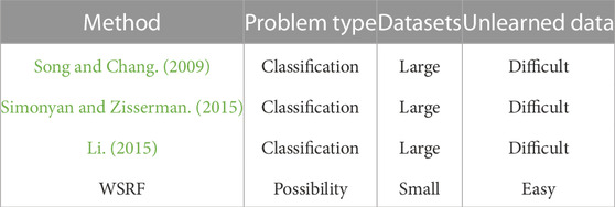
TABLE 7. Different characteristics of comparison methods.

Experiments were conducted on incipient faults that happened in the distribution line. Events are selected from the database containing 400 events, repeated 10 times, and the average value of Accuracy, Precision, Recall, and F1 are shown in Table 8. WSRF achieves good results in Accuracy, Precision, Recall, and F1. The Accuracy is 0.945, far more than the other three methods. The lowest Precision rate is 0.887, and the lowest Recall rate is 0.908. F1 also achieves 0.938. Song and Chang. (2009), Simonyan and Zisserman. (2015); Li. (2015) all achieve good results in Recall, but Precision is lower than WSRF. Accuracy in Song and Chang. (2009) is also lower than WSRF. F1 of the three methods is not good. They reach 0.566, 0.180, and 0.278 respectively, far lower than the WSRF’s 0.938. Simonyan and Zisserman. (2015) and Li. (2015) are far lower than WSRF in terms of Accuracy.

TABLE 8

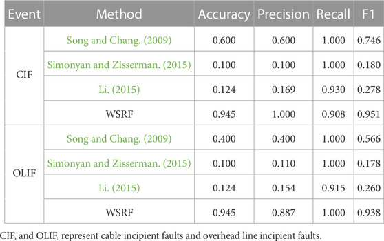
TABLE 8. Results for classification in different methods.

In addition, we show the distribution of F1 in ten experiments to comprehensively score the four methods. The results are shown in Figure 11. The F1 obtained by Song and Chang. (2009) on cable incipient faults is from 0.596 to 0.824 and that on overhead line incipient faults is from 0.431 to 0.730. Simonyan and Zisserman. (2015) scores lower than 0.3 in both two incipient faults. Li. (2015) obtains F1 from 0.05 to 0.5 on cable incipient faults. The score on overhead line incipient faults is from 0.17 to 0.44. WSRF is better than the three methods in these two kinds of fault identification. WSRF obtains the score from 0.909 to 1 on cable incipient faults identification and from 0.889 to 1 on overhead lines. Some conclusions are made from the comparison. Song and Chang. (2009) misclassifies some incipient fault events, but its performance is not bad. Simonyan and Zisserman. (2015) and Li. (2015) misclassify many incipient fault events so that they can not be used to identify incipient faults in the distribution network. In contrast, WSRF has better performance in the identification of incipient faults.

FIGURE 11

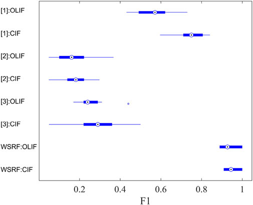
FIGURE 11. F1 of different methods. CIF: Cable incipient fault. OLIF: Overhead line incipient fault. [1]: The method from Song and Chang. (2009) [2]: The method from Simonyan and Zisserman. (2015). [3]: The method from Li. (2015).

WSRF can learn image features in high-dimensional space to compare the similarity of waveforms, rather than learn features corresponding to the label as traditional machine learning. This method can provide a positive result when facing a fault image that has high similarity with an incipient fault. At the same time, it also shows that the possibility of an incipient failure is large. In this way, few samples should be used to support incipient faults classification. Similarly, Song and Chang. (2009) also learns image features in high-dimensional space and classifies them according to these features. For the fault that has been learned before, Song and Chang. (2009) performs well. Unlike WSRF, Song and Chang. (2009) performs poorly on those images that have not been learned in the training set, and the result of the classification function of such images mapped to high-dimensional space is no recognition. Simonyan and Zisserman. (2015) searches features of the waveform from raw data and needs numerous examples to determine network weights. When Simonyan and Zisserman. (2015) is trained with small amounts of data, the result is relatively poor. The same is for Simonyan and Zisserman. (2015), Li. (2015) extracts common features through a large amount of data training. Due to its strong self-adaptive and mapping ability, it has the shortcomings of fast convergence speed and is easy to fall into local optimum in itself. Therefore, the performance of classification is very inferior.

6 Conclusion

This paper proposes WSRF to identify incipient faults in distribution networks. Results illustrate that we can have a feature matrix through feature extraction and calculate the similarity by searching the feature space. The proposed disassembled filters method not only has a good influence on feature extraction but also demonstrates the possibility of using the initial weights to help the comparison with high Accuracy. After learning to compare the similarity of the waveform, we develop a method to split the waveform into several segments. We recognize incipient faults through the similarity of segments and the relation between each other. The results show that WSRF has higher Accuracy than previous methods in identifying incipient faults.

Experiments show that WSRF outperforms the other three classifiers for this task. However, SCN still needs hundreds of data for training and testing. It is a challenge to obtain the high Accuracy of the model with an extremely small training set.

Data availability statement

The raw data supporting the conclusions of this article will be made available by the authors, without undue reservation.

Author contributions

XT carried out the main research tasks and wrote the full manuscript, and QC proposed the original idea, carried out the whole research, analyzed the results and checked the whole manuscript. YW gave constructive comments and revised the manuscript. YS contributed to data processing and to writing and summarizing the proposed ideas. DL participated in preparing the manuscript and provided technical support throughout. All authors read and approved the final manuscript.

Funding

This work was supported by the National Key Research and Development Program (No. 2018YFB2100100).

Conflict of interest

The authors declare that the research was conducted in the absence of any commercial or financial relationships that could be construed as a potential conflict of interest.

Publisher’s note

All claims expressed in this article are solely those of the authors and do not necessarily represent those of their affiliated organizations, or those of the publisher, the editors and the reviewers. Any product that may be evaluated in this article, or claim that may be made by its manufacturer, is not guaranteed or endorsed by the publisher.

References

Cui, Q., El-Arroudi, K., and Weng, Y. (2019). A feature selection method for high impedance fault detection. IEEE Trans. Power Deliv. 34, 1203–1215. doi:10.1109/TPWRD.2019.2901634

CrossRef Full Text | Google Scholar

Cui, T., Dong, X., Bo, Z., and Richards, S. (2008). “Integrated scheme for high impedance fault detection in mv distribution system,” in IEEE/PES Transmission and Distribution Conference and Exposition, Bogota, 13-15 August 2008 (IEEE). doi:10.1109/TDC-LA.2008.4641708

CrossRef Full Text | Google Scholar

Elkalashy, N. I., Lehtonen, M., Darwish, H. A., Taalab, A. I., and Izzularab, M. A. (2008). Dwt-based detection and transient power direction-based location of high-impedance faults due to leaning trees in unearthed mv networks. IEEE Trans. Power Deliv. 23, 94–101. doi:10.1109/TPWRD.2007.911168

CrossRef Full Text | Google Scholar

Ghaderi, A., Mohammadpour, H. A., Ginn, H. L., and Shin, Y. (2015). High-impedance fault detection in the distribution network using the time-frequency-based algorithm. IEEE Trans. Power Deliv. 30, 1260–1268. doi:10.1109/TPWRD.2014.2361207

CrossRef Full Text | Google Scholar

Guo, M., Zeng, X., Chen, D., and Yang, N. (2018). Deep-learning-based Earth fault detection using continuous wavelet transform and convolutional neural network in resonant grounding distribution systems. IEEE Sensors J. 18, 1291–1300. doi:10.1109/JSEN.2017.2776238

CrossRef Full Text | Google Scholar

Jannati, M., Vahidi, B., and Hosseinian, S. H. (2019). Incipient faults monitoring in underground medium voltage cables of distribution systems based on a two-step strategy. IEEE Trans. Power Deliv. 34, 1647–1655. doi:10.1109/TPWRD.2019.2917268

CrossRef Full Text | Google Scholar

Kasztenny, B., Voloh, I., Jones, C. G., and Baroudi, G. (2008). “Detection of incipient faults in underground medium voltage cables,” in 61st Annual Conference for Protective Relay Engineers, College Station, TX, USA, 01-03 April 2008 (IEEE), 349–366. doi:10.1109/CPRE.2008.4515065

CrossRef Full Text | Google Scholar

Kim, C., Bialek, T., and Awiylika, J. (2013). An initial investigation for locating self-clearing faults in distribution systems. IEEE Trans. Smart Grid 4, 1105–1112. doi:10.1109/TSG.2012.2231442

CrossRef Full Text | Google Scholar

Kim, C. J., and Bialek, T. O. (2011). “Sub-cycle ground fault location — Formulation and preliminary results,” in IEEE/PES Power Systems Conference and Exposition, Phoenix, AZ, USA, 01-03 April 2008 (IEEE), 1–8. doi:10.1109/PSCE.2011.5772482

CrossRef Full Text | Google Scholar

Kulkarni, S., Allen, A. J., Chopra, S., Santoso, S., and Short, T. A. (2010). “Waveform characteristics of underground cable failures,” in IEEE PES General Meeting, Minneapolis, MN, USA, 25-29 July 2010 (IEEE), 1–8. doi:10.1109/PES.2010.5590158

CrossRef Full Text | Google Scholar

Kulkarni, S., Santoso, S., and Short, T. A. (2014). Incipient fault location algorithm for underground cables. IEEE Trans. Smart Grid 5, 1165–1174. doi:10.1109/TSG.2014.2303483

CrossRef Full Text | Google Scholar

Lake, B. M. (2014). Towards more human-like concept learning in machines: Compositionality, causality, and learning-to-learn. Computer Science, 211–220.

Google Scholar

Li, Y. Q. (2015). Face recognition algorithm based on improved bp neural network. Int. J. Secur. its Appl. 9, 175–184. doi:10.14257/ijsia.2015.9.5.18

CrossRef Full Text | Google Scholar

Liu, P., and Huang, C. (2018). Detecting single-phase-to-ground fault event and identifying faulty feeder in neutral ineffectively grounded distribution system. IEEE Trans. Power Deliv. 33, 2265–2273. doi:10.1109/TPWRD.2017.2788047

CrossRef Full Text | Google Scholar

Michalik, M., Rebizant, W., Lukowicz, M., Lee, S. J., and Kang, S. H. (2006). High-impedance fault detection in distribution networks with use of wavelet-based algorithm. IEEE Trans. Power Deliv. 21, 1793–1802. doi:10.1109/TPWRD.2006.874581

CrossRef Full Text | Google Scholar

Moghe, R., Mousavi, M. J., Stoupis, J., and McGowan, J. (2009). “Field investigation and analysis of incipient faults leading to a catastrophic failure in an underground distribution feeder,” in IEEE/PES Power Systems Conference and Exposition, Seattle, WA, USA, 15-18 March 2009 (IEEE), 1–6. doi:10.1109/PSCE.2009.4840203

CrossRef Full Text | Google Scholar

Mohsenian-Rad, H. (2022). Smart grid sensors: Principles and applications. Cambridge: Cambridge University Press.

Google Scholar

Morid, M. A., Borjali, A., and Fiol, G. D. (2021). A scoping review of transfer learning research on medical image analysis using ImageNet. Comput. Biol. Med. 128, 104115. doi:10.1016/j.compbiomed.2020.104115

PubMed Abstract | CrossRef Full Text | Google Scholar

Mousavi, M. J., and Butler-Purry, K. L. (2010). Detecting incipient faults via numerical modeling and statistical change detection. IEEE Trans. Power Deliv. 25, 1275–1283. doi:10.1109/TPWRD.2009.2037425

CrossRef Full Text | Google Scholar

Radojevic, Z., Terzija, V., Preston, G., Padmanabhan, S., and Novosel, D. (2013). Smart overhead lines autoreclosure algorithm based on detailed fault analysis. IEEE Trans. Smart Grid 4, 1829–1838. doi:10.1109/TSG.2013.2260184

CrossRef Full Text | Google Scholar

Sarlak, M., and Shahrtash, S. M. (2013). High-impedance faulted branch identification using magnetic-field signature analysis. IEEE Trans. Power Deliv. 28, 67–74. doi:10.1109/TPWRD.2012.2222056

CrossRef Full Text | Google Scholar

Sedighi, A. R., Haghifam, M. R., Malik, O., and Ghassemian, M. H. (2005). High impedance fault detection based on wavelet transform and statistical pattern recognition. IEEE Trans. Power Deliv. 20, 2414–2421. doi:10.1109/TPWRD.2005.852367

CrossRef Full Text | Google Scholar

Sidhu, T. S., and Xu, Z. (2010). Detection of incipient faults in distribution underground cables. IEEE Trans. Power Deliv. 25, 1363–1371. doi:10.1109/TPWRD.2010.2041373

CrossRef Full Text | Google Scholar

Simonyan, K., and Zisserman, A. (2015). “Very deep convolutional networks for large-scale image recognition,” in International Conference on Learning Representations (ICLR), Kuala Lumpur, Malaysia, 03-06 November 2015 (IEEE), 1–14.

Google Scholar

Song, K., and Chang, Y. L. (2009). Research and design of image feature recognition classifier based on svm. Second Int. Conf. Intelligent Comput. Technol. Automation 1, 666–669. doi:10.1109/ICICTA.2009.166

CrossRef Full Text | Google Scholar

Stringer, N., and Kojovic, L. (2001). Prevention of underground cable splice failures. IEEE Trans. Industry Appl. 37, 230–239. doi:10.1109/28.903154

CrossRef Full Text | Google Scholar

Xiong, S., Liu, Y., Fang, J., Dai, J., Luo, L., and Jiang, X. (2020). Incipient fault identification in power distribution systems via human-level concept learning. IEEE Trans. Smart Grid 11, 5239–5248. doi:10.1109/TSG.2020.2994637

CrossRef Full Text | Google Scholar

Xu, W. (2018). “Electric signatures of power equipment failures,” in Transmission & distribution committee power quality subcommittee (IEEE Power & Energy Society).

Google Scholar

Yosinski, J., Clune, J., Bengio, Y., and Lipson, H. (2014). How transferable are features in deep neural networks? arXiv.

Google Scholar

Zeiler, M. D., and Fergus, R. (2013). Visualizing and understanding convolutional networks. arXiv.

Google Scholar

Zhang, W., Jing, Y., and Xiao, X. (2016). Model-based general arcing fault detection in medium-voltage distribution lines. IEEE Trans. Power Deliv. 31, 2231–2241. doi:10.1109/TPWRD.2016.2518738

CrossRef Full Text | Google Scholar

Zhang, W., Xiao, X., Zhou, K., Xu, W., and Jing, Y. (2017). Multicycle incipient fault detection and location for medium voltage underground cable. IEEE Trans. Power Deliv. 32, 1450–1459. doi:10.1109/TPWRD.2016.2615886

CrossRef Full Text | Google Scholar

Zhou, C., Zhou, N., Pan, S., Wang, Q., Li, T., and Zhang, J. (2015). “Method of cable incipient faults detection and identification based on wavelet transform and gray correlation analysis,” in IEEE Innovative Smart Grid Technologies - Asia (ISGT ASIA), Bangkok, Thailand, 03-06 November 2015 (IEEE), 1–5. doi:10.1109/ISGT-Asia.2015.7387146

CrossRef Full Text | Google Scholar