Quality control algorithm of wind speed monitoring data along high-speed railway

1 Introduction

Strong winds are one of the biggest meteorological threats to the safety and operation of high-speed rail. A strike of strong wind on the high-speed rail during normal operation will cause it to derail or overturn in a few seconds (Zhang et al., 2020). As the acquisition, transmission, and storage of the wind speed data are disturbed by various factors, the quality of the second-level wind speed data is greatly reduced. This hinders the scientific assessment of high-speed rail driving safety. The quality control (QC) of the real-time observation data for the second-level wind speed ensures data accuracy. In this way, monitoring can be accurate, and early warning is possible. The QC of the historical observation data for the second-level wind speed can keep the data complete and accurate. The data can serve as the basis for the study of high-speed rail driving safety, contributing to the early warning of strong wind and the optimal layout of monitoring stations.

In recent years, scholars from China and other countries have conducted extensive research on the QC algorithm of meteorological observation data. Their studies focus on the single-station QC algorithm, built from the time dimension of the wind speed observation data, and the multi-station interconnection QC algorithm, built from the spatial dimension. The literature review of the first study direction (i.e., the one from the time dimension) can be summarized as follows: Jiménez et al. (2010) evaluated the quality of wind speed and direction through an extreme value check, a time consistency check, and time series homogenization. Then, he analyzed and corrected the abnormal data in the dataset. Tian et al. (2020) proposed a random sampling-arithmetic average method for the QC of the meteorological observation data. This method is based on random observation, which can effectively improve the quality of the meteorological observation data. Salvação et al. (2022) used weather research forecasting, a regional atmospheric model, to improve wind datasets. The model combines its predictions with remotely sensed wind observations in enhanced wind speed analyses that lead to blended winds. Xiong et al. (2017) proposed a new QC method based on gene-expression programming (GEP) to identify potential outliers in the surface hourly temperature observations. Compared to the spatial regression test (SRT) and inverse distance weighting (IDW), GEP and SRT can generate results better than IDW in all cases. To control the quality of wind speed observation data, Shen et al. (2021) established a correlation function between the target station and the reference station and introduced the Standard Normal Homogeneity Test (SNHT) into the QC. Estévez et al. (2018) the weight estimated via the distance. or correlation coefficient between the observation stations to control the quality of temperature observation data from a spatial perspective. His method can identify doubtful values in temperature observation data and improve data accuracy. Considering the limitations of current QC methods in different regions and on multiple time scales, the kernel regression algorithm is applied to the QC of surface air temperature observations. Ye et al. (2020) improved the kernel regression (IKR) method based on an adaptive algorithm and particle swarm optimization. The RainGaugeQC scheme described in this study aims to provide real-time QC of the telemetric rain gauge data. It consists of several checks: detection of exceedance of the natural limit and climate-based threshold and the conformity checking of rain gauge and radar observations, consistency checking of time series from heated and unheated sensors, and spatial consistency checking of adjacent gauges. The approach proposed by Ośródka et al. (2022) focused on the reliability assessment of individual rain gauge observations.

In short, the studies on the QC of meteorological observation data focused more on the temperature and precipitation and less on the wind speed. Even those focusing on wind speed observation data only explore minute-level meteorological stations. Their wind-speed studies lacked second-level observation data that were non-stationary and non-linear. Therefore, this study proposed a QC algorithm that combined CNN, LSTM, and IF for the second-level wind speed observation data. The data were from five meteorological observation stations along a high-speed railway in China. The method provides sufficient basic data for the research on high-speed rail driving safety.

2 Data

Meteorological observation stations along a high-speed railway in China have different geographical environments. Therefore, this study selects five stations to collect the second-level wind speed observation data (stations 1, 2, 3, 4, and 5). The locations of the five stations are shown in Figure 1. All the second-level wind speed observation data from the five target stations come from ultrasonic anemometers along the railway. The anemometers are arranged on both sides of the track. These data are susceptible to disturbances from the monitoring environment and passing trains. Station 1 is beside the Yangtze River; Station 2 is in the city; Station 3 is in the hills; Station 4 is in the plain; and Station 5 is beside a lake. Data from 2018 were selected for the QC research to keep the integrity of the wind speed observation data on the time scale. The data have passed basic QC checks, such as the extreme value and format checks. Being accurate second-level observation data for wind speed, it has already eliminated obvious gross errors.

FIGURE 1

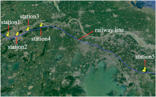
FIGURE 1. Geographical location distribution of the five stations.

3 Materials and methods

3.1 CNN

The convolutional neural network (CNN) model, whose structure is shown in Figure 2, adopts local connectivity and weight sharing, which can map the original data into high-dimensional data for training and effectively extract the features (Dua et al., 2021). In the convolutional layer, the local connectivity and weight sharing greatly reduce the number of parameters in the training process and improve the model’s training speed. This helps the model efficiently extract the original data features. In the pooling layer, the abstract understanding of the original data and the drop of the feature dimension effectively reduce the number of training parameters. Moreover, the model overfitting degree decreases with more efficient extraction of features (Kattenborn et al., 2021; Moolchandani et al., 2021). Compared to traditional neural networks, the main advantage of CNNs is that they can automatically detect important features without the help of human supervision. For example, given pictures of cats and dogs, it can learn the key features of each class by itself. In addition, the number of parameters required for training reduces significantly as all the features have been extracted already.

FIGURE 2

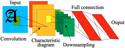
FIGURE 2. CNN structure.

3.2 LSTM

The recurrent neural network (RNN) can only obtain information from closer sequences than from earlier ones. When dealing with long sequence data, it often loses information from the earlier sequences (Chang et al., 2019; Sherstinsky, 2020; Lindemann et al., 2021). Therefore, the problem of RNN is its short-term memory due to the gradient vanishing of RNN units. Long short-term memory (LSTM) solves this problem by introducing the gate mechanism, which includes the forget gate, the input gate, the output gate, and the cell state.

Each LSTM unit is calculated as follows.

3.2.1 Forget gate

The last time’s output value and the current input value are calculated to obtain the output value of the forget gate, as shown in Eq. 1:

$f_t=\sigma \left(w_f.\left[h_{t-1},x_t\right]+b_f\right),(1)$

where $f_t$ is the forget gate, $\bullet$ is the dot product of two vectors, $\sigma$ is the $sigmoid$, $h_{t-1}$ is the unit at the previous time, $w$ is the weight, $x_t$ is the input vector at the time $t$, and $b$ is the bias vector.

3.2.2 Input gate

The last time’s output value and the current input value are entered into the input gate to obtain the output value and the candidate cell state of the input gate as follows:

$i_t=\sigma \left(w_t\left[h_{t-1},x_t\right]+b_i\right),(2)$

$c_t\%=\tanh \left(w_c\left[h_{t-1},x_t\right]+b_c\right),(3)$

where $i_t$ is the input door, $c_t\%$ is the cell state at the current time, and $\tanh \left(\bullet \right)$ is the hyperbolic tangent activation function.

3.2.3 Update of the current cell state

The current cell state is the product of the previous cell state and the forget gate, plus the product of the current cell state and the input gate as follows:

${\mathrm{c}}_t=f_t\bullet {\mathrm{c}}_{t-1}+i_t\bullet c_t\%,(4)$

where $i_t$ is the input door and $c_t\%$ is the current cell state.

3.2.4 Output gate

The output $t$ and input $x_t$ are entered into the input value of the gate as time $t$ to obtain the output gate as follows:

$o_t=\sigma \left(w_o\cdot \left[h_{t-1},x_t\right]+b_o\right),(5)$

$h_t=o_t\bullet \tanh \left(c_t\right),(6)$

where $\tanh \left(\bullet \right)$ is the hyperbolic tangent activation function, $c_t$ is the cell state of the hidden layer at the time $t$, and $o_t$ is the output gate.

3.3 IF

The basic principle of isolation forest (IF) is to divide the data space into two subspaces with a random hyperplane. The subspace will further divide until there is only one data node in each subspace, forming the IF (Lesouple et al., 2021; Zolfaghari and Golabi, 2021).

For a dataset with $n$ data points, the isolation tree has a maximum height of $n-1$ and a minimum height of $\log \left(n\right)$. IF determines whether the datum $x$ is an outlier based on the path $h\left(x\right)$, the length from the leaf node $x$ to the root node. The maximum possible height of the path $h\left(x\right)$ increases linearly with $n$, and the mean possible height increases with $\log \left(n\right)$. Given the similarity between the isolation tree and the binary search tree, $h\left(x\right)$ is normalized using the following equations:

$s\left(x,n\right)=2^{\frac{E\left(h\left(x\right)\right)}{c\left(n\right)}},(7)$

$c\left(n\right)=2H\left(n-1\right)-\left(2\frac{\left(n-1\right)}{n}\right),(8)$

$h\left(k\right)=\ln \left(k\right)+0.577,(9)$

where $s\left(x,n\right)$ is the anomaly score of node $x$, $E\left(h\left(x\right)\right)$ is the expected value of the height $h\left(x\right)$ of node $x$ on multiple isolation trees, $c\left(n\right)$ is obtained based on the average search length (ASL) in the case of search failure, and 0.577 is the Euler–Mascheroni constant. Eq. 7 reflects that the anomaly score $s\left(x,n\right)$ is the monotone decreasing function of $h\left(x\right)$, with a value range of $\left[\mathrm{0,1}\right]$. The closer the score is to 1, the greater the probability of the outlier. There is no obvious outlier in the whole dataset if the score of most data is close to 0.5.

3.4 CNN–LSTM–IF

Based on the non-stationary and non-linear characteristics of second-level wind speed observation data and considering the advantages of the algorithms mentioned previously, this study proposes a QC algorithm that combines CNN, LSTM, and IF. It is used for the second-level wind speed observation data of five meteorological observation stations along a high-speed railway in China. The detailed CNN-LSTM-IF flow is as follows:

Step 1. Select the measured second-level wind speed $x=\left(x_1,x_2,x_3,\dots {x_{m+}}_n\right)$ of the target station.

Step 2. Use CNN to convolute the measured second-level wind speed $x=\left(x_1,x_2,x_3,\dots {x_m}_{+n}\right)$ to extract the features of the original data and obtain the convolved feature $\widehat{y}=\left({\widehat{y}}_1,{\widehat{y}}_2,{\widehat{y}}_3,\dots {\widehat{y}}_{m+n}\right)$.

Step 3. Input the extracted feature $y=\left(y_1,y_2,y_3,\dots y_n\right)$ to the LSTM for a single-step forecast with a window of size $m$ to obtain the forecast second-level wind speed $y=\left(y_1,y_2,y_3,\dots y_n\right)$. Then, obtain the corresponding forecast residual $E=\left(E_1,E_2,E_3,\dots E_n\right)$.

Step 4. Input the forecast residual $E=\left(E_1,E_2,E_3,\dots E_n\right)$ into IF for outlier detection.

Step 5. If the forecast residual is detected as an outlier, correct the outlier of the corresponding position with the linear interpolation; otherwise, repeat Step 1, Step 2, Step 3, and Step 4 until the end.The detailed CNN–LSTM–IF flow is shown in Figure 3.

FIGURE 3

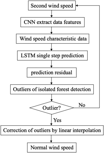
FIGURE 3. CNN–LSTM–IF flow.

3.5 Evaluation indicators

The root mean square error (RMSE) was used to show the difference between measured and predicted values and reflect the performance of the forecast model. The error-detecting rate, type I error, and type II error were adopted to measure the error-detecting capability of the model. Among the three indicators, the error-detecting rate is the ratio of the number of correctly detected doubtable values to the number of all doubtable values; type I error is the ratio of normal values that have been incorrectly detected as doubtable values; and type II error is the ratio of doubtable values that have been incorrectly detected as normal values (Xiong et al., 2022).

Support vector regression (SVR) was used as the comparison method to test the performance of the proposed method. SVR is a data mining method based on statistical theory. As an extension of the SVM, it is designed to handle regression analysis problems. The SVR structure (Figure 1) is similar to that of the ANN model. The input and output layers are connected by a hidden layer, which can be calculated automatically based on the dataset (Inapakurthi and Mitra, 2022).

4 Results and analysis

This study used CNN to extract the original data features. The extracted features were then input to the LSTM for the single-step forecast to obtain the forecast residual. Then, the forecast residual was input into the IF for outlier detection. Finally, the results of the CNN–LSTM, LSTM, and SVR were analyzed separately to compare their forecast performance and error-detecting capabilities.

4.1 Analysis of forecast performance

This study used the forecast residual to detect abnormal second-level wind speed. Therefore, CNN–LSTM, LSTM, and SVR were first compared based on their forecast performances. The test dataset was the second-level wind speed observation data from five meteorological observation stations along a high-speed railway in China in 2018. The average RMSE of the three algorithms for all days in the corresponding season and the RMSE of each algorithm in the corresponding season were derived. The RMSE of the three algorithms is shown in Figure 4.

FIGURE 4

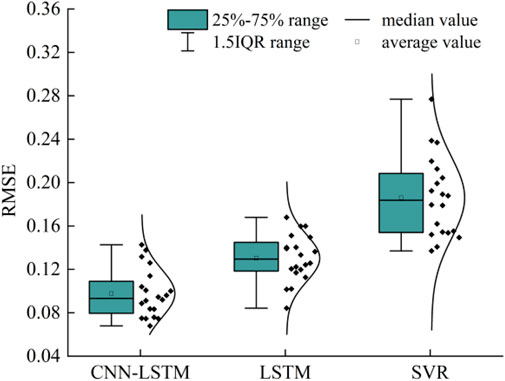
FIGURE 4. RMSE of the three algorithms.

Figure 4 shows that the medians (0.1, 0.13, and 0.18) and the means (0.1, 0.13, and 0.18) of the RMSE of CNN–LSTM in different seasons across the five stations are minimal, indicating a high forecast performance of CNN–LSTM. The CNN–LSTM has the densest indicator distribution among the three algorithms, with an RMSE of 0.07–0.15. This indicates that the CNN–LSTM has high robustness and accuracy. The RMSE obtained by CNN–LSTM is more concentrated at a low value. The densest indicator distribution results show that the proposed method performs better than other methods by yielding good results for different cases. Compared to the other two algorithms, the CNN–LSTM can better extract the features of wind speed observation data. With CNN, the algorithm can map the high-dimensional data into the low-dimensional data. After the extracted features are entered into the LSTM for a single-step forecast, the LSTM’s strong time-series memory supports the forecast of the wind speed observation data in different terrains and seasons.

4.2 Analysis of error-detecting capability

CNN–LSTM–IF is good at detecting abnormal observation data of second-level wind speed. This study used controlled variables to demonstrate its advantages. The outlier detection methods based on forecast residuals were combined with single-step forecast algorithms. In other words, IF was combined with CNN-LSTM, LSTM, and SVR, respectively. Moreover, the second-level wind speed observation data of five meteorological observation stations along a high-speed railway in China in 2018 were used as the test dataset. The average RMSE of the three algorithms for all days in the corresponding season and the RMSE of each algorithm in the corresponding season were derived. The RMSEs of the three algorithms are shown in Figure 4. The error-detecting indicators of CNN–LSTM–IF, LSTM–IF, and SVR–IF are shown in Figure 5.

FIGURE 5

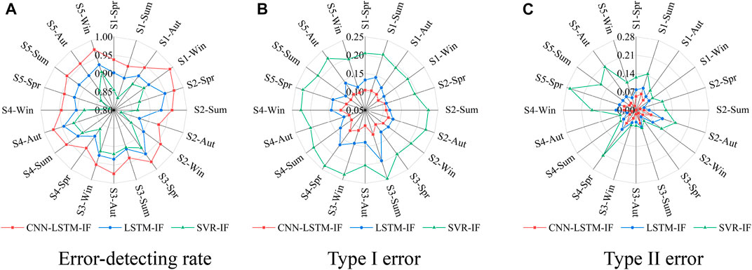
FIGURE 5. Comparison of the error-detecting capability of the three algorithms: (A) Error-detecting rate, (B) Type I error, (C) Type II error [S1-5 is short for section 1-5].

Figure 5 shows the size distribution of the error-detecting indicators of the three algorithms. It is basically the same in different seasons. CNN–LSTM–IF has the best error-detecting indicators, with the error-detecting rate, type I error, and type II error being approximately 0.95, 0.1, and 0.05, respectively. LSTM–IF has the second-best error-detecting indicators, with the error-detecting rate, type I error, and type II error being approximately 0.91, 0.12, and 0.09, respectively. SVR-IF has the worst error-detecting indicators, with the error-detecting rate, type I error, and type II error being approximately 0.88, 0.2, and 0.12, respectively. Therefore, the error-detecting capability of CNN–LSTM–IF is better than that of the other two algorithms. As the five stations are in different regions, they may be affected by the regional microclimate. In different seasons, their error-detecting capability may change. Specifically, Station 1 has the lowest ability to detect errors in the summer because of the prevailing summer winds and complex wind speed fluctuations (Zeng et al., 2018). Station 2’s ability to detect errors becomes the weakest in the fall due to the frequent strong autumn winds. Station 3’s ability to detect error is the weakest in summer because the wind speed in the summer varies significantly as temperature changes, especially at extremely high temperatures. Station 4’s error-detecting capability is the worst in spring when the transit of cold air causes obvious fluctuations in wind speed. The ability of Station 5 to detect errors drops most in the winter, as atmospheric circulation generates strong winter winds.

To further verify the differences among the three algorithms (CNN–LSTM, LSTM, and SVR) in detecting abnormal observation data of second-level wind speed, they were used for single-step forecasts on different data types. The reasons for their different error-detecting capabilities were analyzed based on the forecast residuals (Figure 6).

FIGURE 6

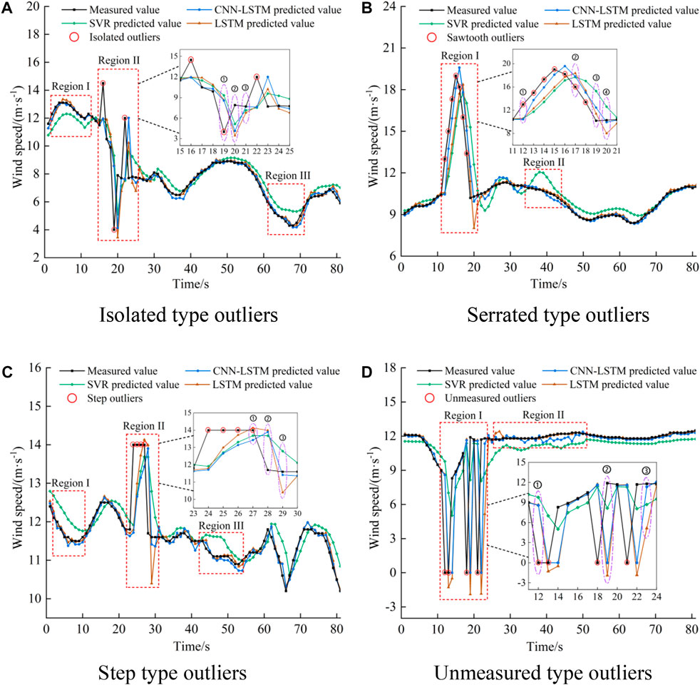
FIGURE 6. Comparison of the difference in error-detecting capability of the three algorithms: (A) Isolated type outliers, (B) Serrated type outliers, (C) Step type outliers, (D) Unmeasured type outliers.

Figures 6A–D show that the SVR has the poorest forecast performance compared to CNN–LSTM and LSTM. It results in large forecast errors in regions I and III of Figure 6A, region II of Figure 6B, regions I and III of Figure 6C, and region II of Figure 6D. If the forecast residual is input into the IF for outlier detection, many normal second-level wind speeds will be detected as abnormal. From the enlarged partial view of region II of Figure 6A and region I of Figure 6D, we can see that the abnormal second-level wind speed in the wind speed sequence for a single-step forecast in the three algorithms results in large forecast residuals. According to region II of Figure 6A and region II of Figure 6D, the normal second-level wind speed is detected as the abnormal second-level wind speed. LSTM and SVR cause large forecast residuals in region III of Figures 6A, D. In comparison, CNN–LSTM has much smaller forecast residuals, as shown in region III of Figure 6A. CNN–LSTM will not detect the normal second-level wind speed as abnormal. From the enlarged partial view of Figures 6B, C, we can see that the three algorithms cause large forecast residuals in region III of Figure 6B and region II of Figure 6C, resulting in the normal second-level wind speed being detected as the abnormal second-level wind speed. The LSTM and SVR cause large forecast residuals in region II of Figure 6B and region III of Figure 6C, resulting in the normal second-level wind speed being detected as the abnormal second-level wind speed. Abnormal second-level wind speed in the wind speed sequence often leads to a large forecast residual at the normal second-level wind speed. However, CNN–LSTM avoids false detection with its unique feature extraction ability. The features of high-dimensional wind speed observation data are extracted by dimension reduction, thus reducing the chance of generating large forecast residuals. Using the forecast residuals generated by the single-step forecast, CNN–LSTM proved to be more suitable for QC.

Moreover, Table 1 shows the performance of different methods for RMSE, error-detecting rate, and the computational burden. As we can see, CNN–LSTM–IF is better than other methods. One explanation is that the proposed algorithm combines the advantages of the CNN, LSTM, and IF algorithms. According to the computational burden index, the time cost is very small despite the complex structure of the proposed algorithm.

TABLE 1

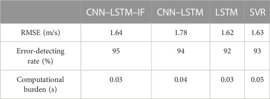
TABLE 1. Performance of different methods for RMSE, error-detecting rate, and the computational burden.

5 Conclusion

Based on the non-stationary and non-linear characteristics of second-level wind speed observation data, this study proposes a QC algorithm that combines CNN, LSTM, and IF. This proposed algorithm is used to detect different types of abnormal second-level wind speed in the second-level wind speed observation data. The observation data are from five meteorological observation stations along a high-speed railway in China. The main conclusions of this paper are as follows:

(1) The CNN–LSTM–IF adopted the CNN–LSTM for single-step forecasting. In the detection of abnormal second-level wind speeds, this algorithm can produce large forecast residuals at abnormal second-level wind speeds and small forecast residuals at normal second-level wind speeds. In this way, false or missed detection is avoided.

(2) The CNN–LSTM–IF constructed the single-station QC algorithm from the time dimension according to the results of tests performed at the five meteorological observation stations along a high-speed railway in China in different seasons. The algorithm had good error-detecting capability and stability in different seasons, with an error detection rate of approximately 0.95.

Data availability statement

The original contributions presented in the study are included in the article/Supplementary Material. Further inquiries can be directed to the corresponding author.

Author contributions

YY: writing of the manuscript; XX: critical review of the manuscript; YC: data collection and data analyses; FY: supervision of the statistical data analyses. All authors contributed to the article and approved the submitted version.

Funding

This research was partially supported by the National Natural Science Foundation of China under Grant Nos. 42205150 and 42205196, the Natural Science Foundation of Jiangsu Province under Grant No. BK20210661, the QingLan Project of the Jiangsu Higher Education Institutions, the Industry-University-Research Cooperation Project, and the Vice General Manager of Science and Technology Project of Jiangsu Province under Grant No. FZ20220065.

Conflict of interest

The authors declare that the research was conducted in the absence of any commercial or financial relationships that could be construed as a potential conflict of interest.

Publisher’s note

All claims expressed in this article are solely those of the authors and do not necessarily represent those of their affiliated organizations, or those of the publisher, the editors, and the reviewers. Any product that may be evaluated in this article, or claim that may be made by its manufacturer, is not guaranteed or endorsed by the publisher.

References

Chang, Z., Zhang, Y., and Chen, W. (2019). Electricity price prediction based on hybrid model of adam optimized LSTM neural network and wavelet transform. Energy 187, 115804. doi:10.1016/j.energy.2019.07.134

CrossRef Full Text | Google Scholar

Dua, N., Singh, S. N., and Semwal, V. B. (2021). Multi-input CNN-GRU based human activity recognition using wearable sensors. Computing 103 (7), 1461–1478. doi:10.1007/s00607-021-00928-8

CrossRef Full Text | Google Scholar

Estévez, J., Gavilán, P., and García-Marín, A. P. (2018). Spatial regression test for ensuring temperature data quality in southern Spain. Theor. Appl. Climatol. 131 (1-2), 309–318. doi:10.1007/s00704-016-1982-8

CrossRef Full Text | Google Scholar

Inapakurthi, R. K., and Mitra, K. (2022). Optimal surrogate building using SVR for an industrial grinding process. Mater. Manuf. Process. 37 (15), 1701–1707. doi:10.1080/10426914.2022.2039699

CrossRef Full Text | Google Scholar

Jiménez, P. A., González-Rouco, J. F., Navarro, J., Montávez, J. P., and García-Bustamante, E. (2010). Quality assurance of surface wind observations from automated weather stations. J. Atmos. Ocean. Technol. 27 (7), 1101–1122. doi:10.1175/2010jtecha1404.1

CrossRef Full Text | Google Scholar

Kattenborn, T., Leitloff, J., Schiefer, F., and Hinz, S. (2021). Review on convolutional neural networks (CNN) in vegetation remote sensing. ISPRS J. photogrammetry remote Sens. 173, 24–49. doi:10.1016/j.isprsjprs.2020.12.010

CrossRef Full Text | Google Scholar

Lesouple, J., Baudoin, C., Spigai, M., and Tourneret, J. Y. (2021). Generalized isolation forest for anomaly detection. Pattern Recognit. Lett. 149 (3), 109–119. doi:10.1016/j.patrec.2021.05.022

CrossRef Full Text | Google Scholar

Lindemann, B., Maschler, B., Sahlab, N., and Weyrich, M. (2021). A survey on anomaly detection for technical systems using LSTM networks. Comput. Industry 131 (3), 103498. doi:10.1016/j.compind.2021.103498

CrossRef Full Text | Google Scholar

Moolchandani, D., Kumar, A., and Sarangi, S. R. (2021). Accelerating CNN inference on ASICs: A survey. J. Syst. Archit. 113, 101887. doi:10.1016/j.sysarc.2020.101887

CrossRef Full Text | Google Scholar

Ośródka, K., Otop, I., and Szturc, J. (2022). Automatic quality control of telemetric rain gauge data providing quantitative quality information (RainGaugeQC). Atmos. Meas. Tech. Discuss. 15 (19), 5581–5597. doi:10.5194/amt-15-5581-2022

CrossRef Full Text | Google Scholar

Salvação, N., Bentamy, A., and Soares, C. G. (2022). Developing a new wind dataset by blending satellite data and WRF model wind predictions. Renew. Energy 198, 283–295. doi:10.1016/j.renene.2022.07.049

CrossRef Full Text | Google Scholar

Shen, C., Zha, J., Wu, J., and Zhao, D. (2021). Centennial-scale variability of terrestrial near-surface wind speed over China from reanalysis. J. Clim. 34 (14), 1–52. doi:10.1175/jcli-d-20-0436.1

CrossRef Full Text | Google Scholar

Sherstinsky, A. (2020). Fundamentals of recurrent neural network (RNN) and long short-term memory (LSTM) network. Phys. D. Nonlinear Phenom. 404, 132306. doi:10.1016/j.physd.2019.132306

CrossRef Full Text | Google Scholar

Tian, S., Zhang, J., Chen, L., Liu, H., and Wang, Y. (2020). Random sampling-arithmetic mean: A simple method of meteorological data quality control based on random observation thought. IEEE Access 8, 226999–227013. doi:10.1109/access.2020.3045434

CrossRef Full Text | Google Scholar

Xiong, X., Jiang, Z., Tang, H., Zhang, Y., and Ye, X. (2022). Research on quality control methods for surface temperature observations via spatial correlation analysis. Int. J. Climatol. 2022 (42), 10268–10284. doi:10.1002/joc.7897

CrossRef Full Text | Google Scholar

Xiong, X., Ye, X., and Zhang, Y. (2017). A quality control method for surface hourly temperature observations via gene-expression programming. Int. J. Climatol. 37 (12), 4364–4376. doi:10.1002/joc.5092

CrossRef Full Text | Google Scholar

Ye, X., Kan, Y., Xiong, X., Zhang, Y., and Chen, X. (2020). A quality control method based on an improved kernel regression algorithm for surface air temperature observations. Adv. Meteorology 2020, 1–15. doi:10.1155/2020/6045492

CrossRef Full Text | Google Scholar

Zeng, X. M., Wang, M., Wang, N., Yi, X., Chen, C., Zhou, Z., et al. (2018). Assessing simulated summer 10-m wind speed over China: Influencing processes and sensitivities to land surface schemes. Clim. Dyn. 50, 4189–4209. doi:10.1007/s00382-017-3868-6

CrossRef Full Text | Google Scholar

Zhang, Y., Pan, G., Chen, B., Han, J., Zhao, Y., and Zhang, C. (2020). Short-term wind speed prediction model based on GA-ANN improved by VMD. Renew. Energy 156, 1373–1388. doi:10.1016/j.renene.2019.12.047

CrossRef Full Text | Google Scholar

Zolfaghari, M., and Golabi, M. R. (2021). Modeling and predicting the electricity production in hydropower using conjunction of wavelet transform, long short-term memory and random forest models. Renew. Energy 170, 1367–1381. doi:10.1016/j.renene.2021.02.017

CrossRef Full Text | Google Scholar