Wind speed forecasting using optimized bidirectional LSTM based on dipper throated and genetic optimization algorithms

1 Introduction

Increasing reliance on renewable energy supplies directly results from the need to meet rising energy demands while mitigating the negative environmental impacts of traditional fossil fuels. Renewable energy options are vital to lessen this impact and lessen reliance on conventional fuels. In particular, nations that have signed the Paris Climate Agreement have committed to lowering their emissions of greenhouse gases. Due to its accessibility and lack of emissions, wind power is gaining popularity. The potential of wind energy has been widely recognized in the previous 2 decades. As the cost to maintain and operate wind turbines drops and their dependability improves, the number of wind farms grows exponentially. Yet, the reliability of wind farms is impacted by the intermittent and variable nature of wind energy (Albalawi et al., 2022; Chen et al., 2022). Therefore, it is becoming increasingly important that wind energy be predictable (Zeng et al., 2020).

There has been a surge in a study on predicting wind speeds in the past decade. Physical, statistical, machine learning, and hybrid forecasting methods are the most common approaches (Shang et al., 2022). To generate mathematical equations, physical approaches draw on concepts from geophysical fluid dynamics and thermodynamics. The NWP (numerical weather prediction system) model underpins most physical approaches. The intricate mathematical design of NPW models makes them extremely time-consuming to compute (Carvalho et al., 2012). Because of this, NPW models are often reserved for long-term forecasting, making them impractical for short-term wind power predictions.

Statistical models assume a linear relationship between observed wind data and wind speed to predict wind speed. While many statistical models can account for linear trends in wind speed and direction, very few can account for the data’s nonlinear characteristics (Fang and Chiang, 2016; Khafaga et al., 2022). The capacity of artificial intelligence (AI) models to understand the input-output connection from historical data has led to their increased adoption in wind forecasting. In particular, AI algorithms decipher nonlinear relationships in the data and spot previously concealed patterns, allowing for accurate value predictions (Doaa et al., 2022; Sun and Jin, 2022). The capacity to update the model in response to new information is another benefit of AI-based models (Demolli et al., 2019). While there are benefits to using a variety of AI techniques, there are also drawbacks to consider (Shang et al., 2022). Consequently, the advantages of several approaches are utilized in hybrid or combination models.

The structure of a renewable energy management system is shown in Figure 1 (Fathima and Palanisamy, 2016). To aid in the routine upkeep and emergency repairs of electrical equipment in a manufacturing facility, farm, or even an entire municipality, an EMS is in place to handle energy control, management, maintenance, and consumption concerns. It can keep tabs on the machinery’s working condition and promptly boost management. For managers of an electrical company, money can be saved and used to increase equipment life by practicing good management. The system may promptly send out an alarm to aid management personnel in monitoring and repair, reducing losses to a minimum in the case of equipment breakdowns or other situations. The EMS may also message the appropriate people when it detects that specific high-energy-use gadgets are getting on in years. Data collection, storage, processing, statistics, query, and analysis, as well as data monitoring and diagnostics, are all possible in a renewable energy management system (REMS) thanks to the employment of programmed control system technology, network communication, and database technology. Figure 1 shows how the EMS accomplishes its monitoring and management aims by dispatching electricity generated by renewable sources in accordance with a projection of that power made using a forecasting model. Per-unit energy consumption and economic and energy efficiency are lowered through centralized monitoring and efficient administration of energy data. In light of this, the model used for making predictions is a vital EMS input.

FIGURE 1

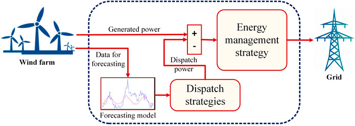
FIGURE 1. The typical architecture of wind speed prediction and power generation system.

Physical, statistical, machine learning, and hybrid models are the most common categories used to categorize methods for predicting wind speed (Shang et al., 2022). To predict wind speed, physical models often use data about the weather, including meteorological characteristics and geographical information. Regarding general-purpose physical models, the numerical weather prediction (NWP) approach is among the most well-known and successful ones. Using the widely-used weather research and forecast (WRF) model, the authors of (Carvalho et al., 2012) evaluate several computational and physical approaches. To provide more accurate estimates of wind speeds at the Earth’s surface, the authors of (Hoolohan et al., 2018) integrate the NWP with the Gaussian process regression. The primary challenges of NWP approaches are the computing demands and the update frequency of forecasts.

The prediction of near-term wind speeds relies heavily on statistical approaches. In their ground-breaking research, authors (Brown et al., 1984) predict wind speed using an autoregressive (AR) model. According to (Torres et al., 2005), the authors indicate the mean hourly wind speed 10 h into the future using the ARMA (autoregressive moving average process) approach. The authors of (Rajagopalan and Santoso, 2009) use this technique similarly to predict wind speed. Their findings suggest their algorithm can reliably estimate speeds within 1 h. For predicting the next hour’s wind speed, the authors of (Sfetsos, 2002) offer an ARIMA (autoregressive integrated moving average) model that considers averages over the previous 10 minutes and hour. Based on the data, it appears that 10-min averages are more reliable. To forecast wind speed up to 2 days in advance, the authors of (Kavasseri and Seetharaman, 2009) investigate fractional-ARIMA models. Wind power generation forecasting is much easier with ARIMA, as demonstrated by the authors of (Eldali et al., 2016). Using a combination of the ARIMA and clustering approaches, the authors of (Akhil et al., 2022) offer a model for predicting wind speed a full year in advance. Short-term predictions of offshore wind speed are shown in (Liu et al., 2021), which presents a seasonal ARIMA model. They evaluate how well-known machine learning methods like the GTU (gated recurrent unit) and the LSTM (long short-term memory) perform in comparison to the ARIMA model (long short-term memory). Their findings suggest that the seasonal ARIMA model performs better than the GTU and the LSTM. Univariate ARIMA is compared with NARX (nonlinear autoregressive exogenous) models by the authors of (Cadenas et al., 2016). The findings demonstrate that the NARX performs better wind speed prediction than the ARIMA.

Nonlinearity in wind data has increased interest in using artificial intelligence systems for predicting wind speeds. For nonlinear data, in particular, ANN (artificial neural network) is an effective technique (Sun and Jin, 2022). The authors of (Cadenas and Rivera, 2009) study short-term wind speed predictions using ANN models. Two-layer ANN appears to perform best in both the learning and prediction phases. The authors of (Dumitru and Gligor, 2017) use a FANN (feedforward neural networks) model to predict daily wind features from historical data. In (Higashiyama et al., 2017), the authors use CNN (convolutional neural networks) to process high-dimensional data for wind forecasting. They suggest a feature extraction technique based on convolutional neural networks to reduce the size of the massive datasets generated by NWP. A further investigation (Yu et al., 2019) uses CNN to predict wind power generation, this time factoring in the wind’s temporal and geographical variations. For their short-term forecast of Estonia’s wind energy output, the authors of (Shabbir et al., 2022) use a recurrent neural network (RNN) algorithm (LSTM). According to their findings, LSTM outperforms SVR (support vector machines) and NAR (neighbor-association recognition) (Nonlinear Autoregressive Neural Networks).

For more precise and efficient wind speed predictions, hybrid and combination models incorporate the best features of many models. As an example, the authors of (Li et al., 2018) use the wavelet transform in predicting to filter out high-frequency data and SVR. To improve the precision of wind power forecasting, the authors of (Liu et al., 2018) suggest a two-stage approach. First, WPD splits wind speed time data into sublayers (Wavelet Packet Decomposition). They use convolutional neural networks (CNNs) and CNNLSTMs (convolutional long short-term memory networks) to create predictions at both high- and low-frequency layers. Hybrid models are a type of model in which an ANN model’s input variables and problem parameters are determined using a different approach. In (Sun and Jin, 2022), for instance, ARIMA is used to identify ANN model input neurons. In (López and Arboleya, 2022), the authors select their input variables using the Pearson Correlation Coefficient (PCC). The authors suggest utilizing these parameters as inputs for LSTM and DNN (Dynamic Neural Networks) models. The authors of (Xiong et al., 2022) use the attention mechanism to prioritize input variables. Data decomposition into subseries is a relatively new method used in hybrid models. For instance, the authors’ decomposition of wind speed data into subseries is performed using a wavelet technique in (Yu et al., 2018). The RNN (recurrent neural networks) and its variations LSTM and GTU are used to extract more nuanced information from low-frequency subseries for forecasting. They found that decomposition, in addition to using hybrid models, improves the reliability of predictions. In (Shang et al., 2022), the authors deconstruct historical wind speed data using CEEMD (complementary ensemble empirical mode decomposition). Then they use SOM (subspace-oriented metric) clustering to organize the resulting data (self-organizing map). To better predict how much energy will be generated by the wind, the authors of (Praveena and Dhanalakshmi, 2018) use a Fuzzy K-Means approach to group together comparable days.

As the most dominant approach used in time series forecasting is the bidirectional long short-term memory (BiLSTM), as it gives promising prediction results, it is noted that this approach needs further improvements to boost its performance. This gap in the performance of the BiLSTM prediction model forms the main motivation for this research. In this research, a new metaheuristic optimization algorithm is proposed for feature selection and for optimizing the parameters of BiLSTM to boost its performance. The feature selection is performed using a new binary algorithm based on hybrid genetic and dipper-throated optimization algorithms. In addition, the continuous version of this algorithm is used to optimize the parameters of the BiLSTM. The proposed model is capable of capturing the data’s long-term variations. The results are assessed using a set of evaluation metrics and a set of statistical tests to confirm its superiority, effectiveness, and statistical difference when compared to other competing models. The main contributions of this work are listed in the following:

• A new optimization algorithm is proposed for optimizing the parameters of BiLSTM.

• A new feature selection algorithm is proposed to select the best features for improving wind speed prediction.

• A comparison between the feature selection results is performed in terms of the proposed feature selection algorithm and the other eight feature selection algorithm.

• A comparison between the results of wind speed prediction using BiLSTM when optimized using the proposed GADTO algorithm and four other optimization algorithms.

• Statistical analysis of the results is presented and discussed to show the significant difference between the proposed and other methods.

The structure of this paper is organized as follows. In Section 2, the proposed method is presented and discussed. Section 3 explains the details of the experimental setup and the computational findings. Section 4 concludes with a brief discussion of the results and suggestions of this work for further study.

2 The proposed methodology

The proposed wind forecasting methodology is shown in the flowchart depicted in Figure 2. In this figure, there are five key phases. The first phase is data preprocessing, in which the dataset is collected and preprocessed to remove outliers and handle missing values, and the data is cleaned. In addition, this phase includes data normalization that helps to eliminate the potential for bias toward outlying numbers. The second phase is feature selection, in which a novel feature selection algorithm is proposed based on the dipper throated and genetic optimization algorithms. The third phase is the optimization of the long short-term memory prediction model. The optimization of this model is applied in terms of the proposed optimization algorithm. The fourth stage is predicting the wind speed using the optimized model. The fifth stage is the evaluation and statistical analysis of the achieved prediction results.

FIGURE 2

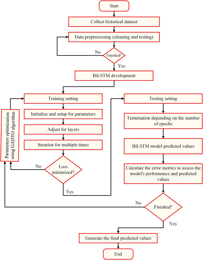
FIGURE 2. The architecture of the proposed methodology.

2.1 Description of the dataset

The benchmark dataset employed in this work is freely available on Kaggle (Fedesoriano, 2022). This dataset contains 6,574 instances in a collection of responses from a set of sensors within a weather station that measures five weather variables. The device was put at 21M in a vacant part of the wind farm. From the beginning of 1961 to the end of 1978, the data were collected for 17 years. Precipitation, high and low temperatures, and the grass’s lowest temperature were supplied daily as recorded by the Ground Truth. Table 1 presents the dataset’s variables and the corresponding description. In addition, the behavior of the variables is shown in the plots of Figure 3, and the histogram of these variables is depicted in Figure 4. These plots give insights into the nature of the variables, which necessitates a robust forecasting model to achieve high prediction results.

TABLE 1

TABLE 1. The variables of the wind speed dataset employed in this research.

FIGURE 3

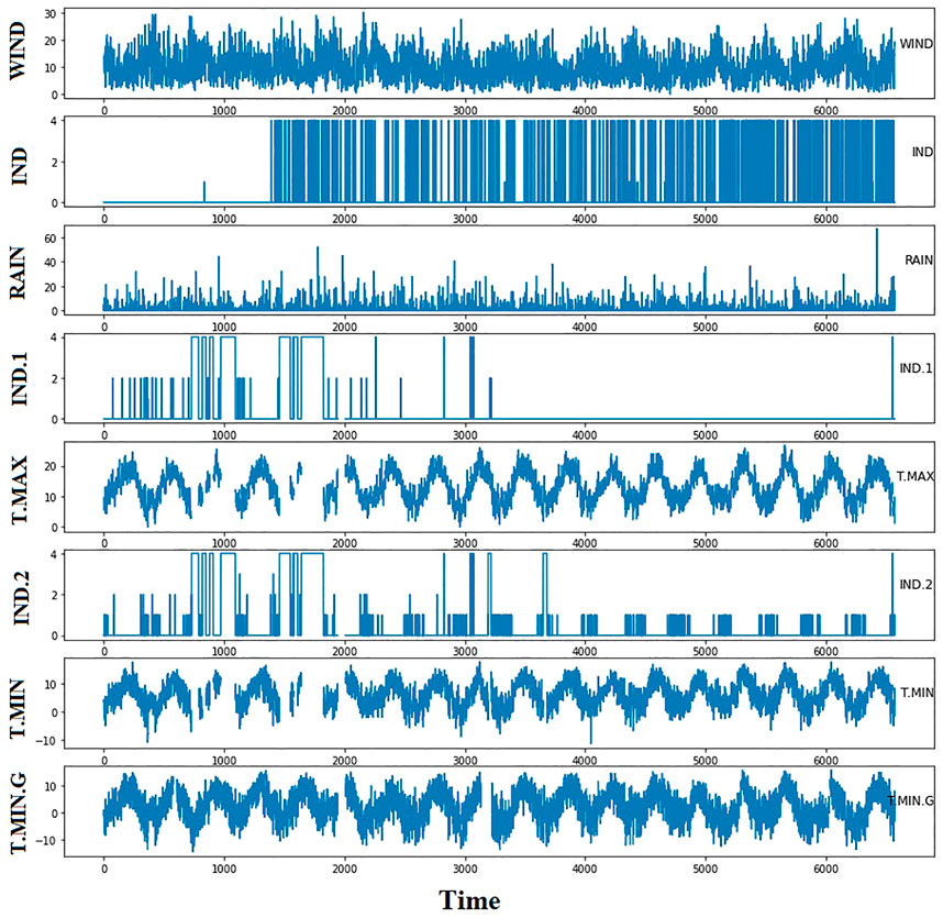
FIGURE 3. The time series of the datset variables in the adopted dataset.

FIGURE 4

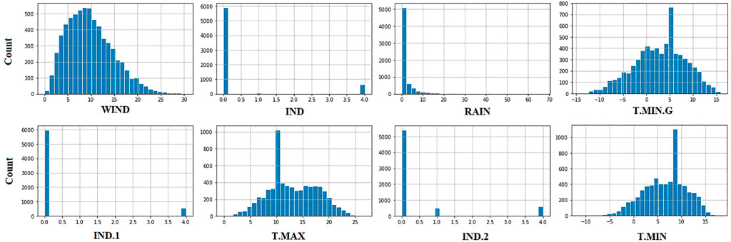
FIGURE 4. Histogram of the dataset variables employed in this research.

2.2 Data preprocessing

Obtaining a reliable prediction model requires preprocessing of the raw data. Removing anomalies from the data, such as outliers and missing values, is necessary. Interpolation of the observed data is used for imputation in time series to replace missing values. In addition, scaling the data into the interval [0, 1] is achieved using min-max normalization. The historical data is then split into training, validation, and testing sets. The machine learning model is constructed from the training set, with already known inputs and outputs. The model’s hyperparameters are tuned with the help of the validation set. The testing set is used for estimating how well a model will do with data that was not used to train it. The training set accounts for 70% of the dataset, the validation set accounts for 10%, and the test set accounts for 20%.

2.3 Long short-term memory (LSTM)

Due to its outstanding potential to preserve sequence information across time, long short-term memory (LSTM) is a complicated computing unit that can achieve better results in sequence modeling applications results from applying LSTM to a wide range of domains show that it can define data connected with time series dependencies and capture the data variance pattern. The bursting and disappearing gradient problem in recurrent neural network (RNN) training may be dealt with by using LSTn. This new sort of neural network was developed to handle the challenges of RNNs in learning these types of long-term incompatibilities. The strongest method for recognizing and altering the long-range context is the LSTM architecture’s built-in memory cells. Three primary gates comprise an LSTM block: the input gate, the forget gate, and the output gate with a memory cell. The cellular states are controlled by gates like these and the sigmoid activation function. In Figure 5, the LSTM cell layout is shown, which includes the LSTM’s essential components, such as the added element level and the multiplication symbol, which stands for the multiplication of the element levels (Abdel Samee et al., 2022; El-Kenawy et al., 2022).

FIGURE 5

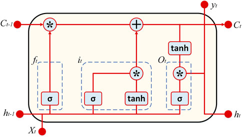
FIGURE 5. The typical architecture of LSTM prediction model.

The input gate determines the magnitude of the values entering the cell and being stored in the processor’s memory (i_t). The information in a memory cell is pruned down to only the necessary bits using a mechanism called a forget gate (f_t), which also determines the percentage of the original values to be retained. The LSTM’s output is activated by the output gate (o_t), and the activated information defines its output. Furthermore, the input node (g_t) acts as an activation vector for cells. The mathematical performance of the LSTM is depicted by the following equations, where h_t is the hidden variable, and sigma is the logistic sigmoid.

$f\left(t\right)=\sigma \left(W_{xf}{x}_t+W_{hf}{h}_{t-1}+W_{cf}{c}_{t-1}+b_f\right)(1)$

$i\left(t\right)=\sigma \left(W_{xi}{x}_t+W_{hi}{h}_{t-1}+W_{ci}{c}_{t-1}+b_i\right)(2)$

$g\left(t\right)=f_t{g}_{t-1}+i_t\mathit{tanh}\left(W_{xg}{x}_t+W_{hg}{h}_{t-1}+b_g\right)(3)$

$o\left(t\right)=\sigma \left(W_{xo}{x}_t+W_{ho}{h}_{t-1}+W_{co}{c}_t+b_o\right)(4)$

$h\left(t\right)=o_t\mathit{tanh}\left(g_t\right)(5)$

2.4 Bidirectional long short-term memory (BiLSTM)

To improve the efficiency of the classification procedure, LSTM is used to develop BiLSTM. As shown in Figure 6, BiLSTM is developed by fusing RNNs with LSTM methods (which provide access to a broad context). Compared to traditional RNNs and time-windowed multilayer perceptrons, BiLSTM networks are quicker and more accurate and beat unidirectional networks like LSTM. In addition, BiLSTM includes extensive information for all phases before and after each step in the specified sequence. Moreover, the LSTM technique calculates the hidden layers in BiLSTM. One distinguishing feature of BiLSTM over LSTM is its ability to process input in both directions, thanks to using two hidden layers that feed their respective outputs into the same output layer (Saeed et al., 2020; Sami Khafaga et al., 2022a; Sami Khafaga et al., 2022b).

FIGURE 6

FIGURE 6. The typical architecture of BiLSTM prediction model.

2.5 Genetic algorithm

The genetic algorithm (GA) optimization is inspired by the genomics operations based on the crossover and mutation process. In this work, the genetic algorithm is hybridized with the DTO algorithm to form the proposed GADTO algorithm which is used in feature selection and parameters optimization of the long short-term memory employed for predicting the wind speed values. One of the main steps of the genetic algorithm is the mutation operator, which produces a new solution with characteristics that differ from those of the parent’s chromosomes. This provides many different solutions rather than just one ideal solution. In this work, we developed a new mutation method for improving the search space exploration. The mutation operation is applied to the positions of the birds of the DTO algorithm to enable them to explore more areas in the search space. The mutation is performed using the following equation.

$P\left(t+1\right)=2*k*z^2-h*P\left(t\right)*\frac{\mathit{cos}\left(P\left(t\right)\right)}{1-\mathit{cos}\left(P\left(t\right)\right.}(6)$

where P(t) and P(t + 1) denote the individual position at iteration t and t + 1, respectively. k is a random number in the range [0, 2], z is a random number in the range of [0, 1] with exponential behavior, and h is a random number in the range (Abdel Samee et al., 2022; Akhil et al., 2022).

2.6 Dipper throated optimization

The optimization process of the dipper throated optimization (DTO) is based on two types of groups of birds, namely, swimming birds and flying birds. These birds are looking for food, so they update their positions (P) and velocities (V) to reach the food efficiently. The following matrices represent the location and velocity of the birds.

$P=\left[\begin{array}{ccccc}\hfill P_{\mathrm{1,1}}\hfill & \hfill P_{\mathrm{1,2}}\hfill & \hfill P_{\mathrm{1,3}}\hfill & \hfill \dots \hfill & \hfill P_{1,d}\hfill \\ \hfill P_{\mathrm{2,1}}\hfill & \hfill P_{\mathrm{2,2}}\hfill & \hfill P_{\mathrm{2,3}}\hfill & \hfill \dots \hfill & \hfill P_{2,d}\hfill \\ \hfill P_{\mathrm{3,1}}\hfill & \hfill P_{\mathrm{3,2}}\hfill & \hfill P_{\mathrm{3,3}}\hfill & \hfill \dots \hfill & \hfill P_{3,d}\hfill \\ \hfill \dots \hfill & \hfill \dots \hfill & \hfill \dots \hfill & \hfill \dots \hfill & \hfill \dots \hfill \\ \hfill P_{m,1}\hfill & \hfill P_{m,2}\hfill & \hfill P_{m,3}\hfill & \hfill \dots \hfill & \hfill P_{m,d}\hfill \end{array}\right](7)$

$V=\left[\begin{array}{ccccc}\hfill V_{\mathrm{1,1}}\hfill & \hfill V_{\mathrm{1,2}}\hfill & \hfill V_{\mathrm{1,3}}\hfill & \hfill \dots \hfill & \hfill V_{1,d}\hfill \\ \hfill V_{\mathrm{2,1}}\hfill & \hfill V_{\mathrm{2,2}}\hfill & \hfill V_{\mathrm{2,3}}\hfill & \hfill \dots \hfill & \hfill V_{2,d}\hfill \\ \hfill V_{\mathrm{3,1}}\hfill & \hfill V_{\mathrm{3,2}}\hfill & \hfill V_{\mathrm{3,3}}\hfill & \hfill \dots \hfill & \hfill V_{3,d}\hfill \\ \hfill \dots \hfill & \hfill \dots \hfill & \hfill \dots \hfill & \hfill \dots \hfill & \hfill \dots \hfill \\ \hfill V_{m,1}\hfill & \hfill V_{m,2}\hfill & \hfill V_{m,3}\hfill & \hfill \dots \hfill & \hfill V_{m,d}\hfill \end{array}\right](8)$

Where P_i,j, refers to the position of the i^th bird in the j^th dimension for i ∈ [1, 2, 3, …, m] and j ∈ [1, 2, 3, …, d], and its velocity in the j^th dimension is indicated by V_i,j. For each bird, the values of the fitness functions f = f₁, f₂, f₃, …, f_n are determined by the following matrix.

$f=\left[\begin{array}{c}\hfill f_1\left(P_{\mathrm{1,1}},P_{\mathrm{1,2}},P_{\mathrm{1,3}},\dots ,P_{1,d}\right)\hfill \\ \hfill f_2\left(P_{\mathrm{2,1}},P_{\mathrm{2,2}},P_{\mathrm{2,3}},\dots ,P_{2,d}\right)\hfill \\ \hfill f_3\left(P_{\mathrm{3,1}},P_{\mathrm{3,2}},P_{\mathrm{3,3}},\dots ,P_{3,d}\right)\hfill \\ \hfill \dots \hfill \\ \hfill f_m\left(P_{m,1},P_{m,2},P_{m,3},\dots ,P_{m,d}\right)\hfill \end{array}\right](9)$

2.7 The proposed optimization algorithm

The steps of the proposed optimization algorithm are presented in Algorithm 1. In these steps, both DTO and GA algorithms are hybridized in a unified algorithm in which the dynamic swapping between the DTO and GA algorithms improves the search space exploration. This algorithm benefits from the mutation step of the GA algorithm to help birds of the DTO algorithm better explore the search space and thus can find the best solution more accurately. In this algorithm, t and T_max refer to the iteration number and the maximum number of iterations, respectively. The values of the parameters r₁, r₂, r₃, K, K₁, K₂, K₃, K₄, K₅, z are selected randomly. P_best and P_Gbest refer to the local and global best solutions.

2.8 Feature selection

The feature selection process eliminates excessive, redundant, and noisy data. The main benefit of the feature selection is that it helps improve the model’s performance as it decreases the dimensionality of the dataset. Since employing raw features might produce ineffective results, optimal feature selection can be essential in providing precise forecasts. Consequently, several techniques employed various feature selection strategies before using the data to train a model (El-kenawy et al., 2022). Relevant features are selected from raw data using the binary version of the proposed optimization algorithm, which is described by the steps presented in Algorithm 2.

Algorithm 1. The proposed GADTO algorithm.

1: Initialize birds’ positions P_i(i = 1, 2, …, n) for n birds, birds’ velocity V_i(i = 1, 2, …, n), objective function f_n, iterations t, T_max, parameters of r₁, r₂, r₃, K, K₁, K₂, K₃, K₄, K₅, z

2: Calculate fitness of f_n for each bird P_i

3: Find best bird position P_best

4: Convert best solution to binary [0, 1]

5: Sett = 1

6: whilet ≤ T_maxdo

7: for(i = 1: i < n + 1)do

8:  if(t%2 == 0)then

9:   if(r₃ < 0.5)then

10:    Update the current swimming bird’s position as: P(i + 1) = P_best(i) − K₁.|K₂.P_best(i) − P(i)|

11:   else

12:    Update the current flying bird’s velocity as: V(i + 1) = K₃V(i) + K₄r₁(P_best(i) − P(i)) + K₅r₂(P_Gbest − P(i))

13:    Update the current flying bird’s position as: P(i + 1) = P(i) + V(i + 1)

14:   end if

15:  else

16:   Mutate birds’ positions using: $P(i+1)=2*K*z^2-h*P(i)*\frac{\mathit{cos}(P(i))}{1-\mathit{cos}(P(i)}$

17:  end if

18: end for

19: Updater₁, r₂, r₃, K, K₁, K₂, K₃, K₄, K₅, z

20: Calculate objective function f_n for each bird P_i

21: Find the best position P_best

22: end while

23: Return the best solution P_Gbest

3 Experimental results

The conducted experiments are classified into two types. The first type is a set of experiments targeting and evaluating the proposed feature selection algorithm. Whereas the second type is a set of experiments that assessed the optimized LSTM model, which is optimized using the proposed GADTO algorithm. This section presents the results achieved by these sets of experiments in addition to the statistical analysis of these results.

3.1 Configuration parameters of optimization algorithms

The conducted experiments include a set of optimization algorithms; namely, standard GA (Immanuel and Chakraborty, 2019) standard DTO (Takieldeen et al., 2022), particle swarm optimization (PSO) (Awange et al., 2018), grey wolf optimization (GWO) (Mirjalili et al., 2014), whale optimization algorithm (WOA) (Mirjalili and Lewis, 2016) and firefly algorithm (FA) (Ariyaratne and Fernando, 2023). The basic configuration parameters of these algorithms are presented in Table 2.

TABLE 2

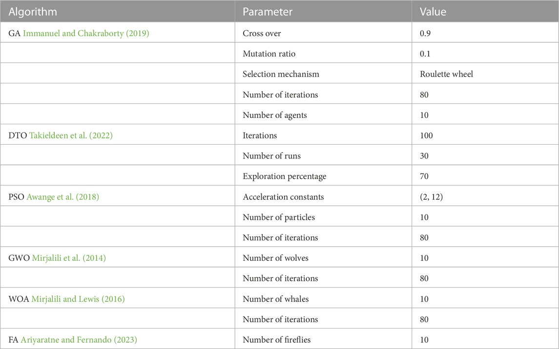
TABLE 2. Configuration parameters of the optimization algorithms.

Algorithm 2. The proposed binary GADTO (bGADTO) algorithm.

1: Initialize the parameters of GADTO algorithm

2: Convert the resulting best solution to binary [0,1]

3: Evaluate the fitness of the resulting solutions

4: Train KNN to assess the resulting solutions

5: Sett = 1

6: whilet ≤ Max_iterationdo

7: Run GADTO algorithm to get best solutions P_best

8: Convert best solutions to binary using the following equation:

$\begin{array}{cc}\hfill & Binary\text{\_}Solution=\left\{\begin{array}{cc}1\hfill & \text{if\hspace{0.17em}}F\left(P_{\mathit{best}}\right)\ge 0.5\hfill \\ 0\hfill & otherwise\hfill \end{array}\right.,\hfill \\ \hfill & F\left(P_{\mathit{best}}\right)=\frac{1}{1+e^{-10\left(P_{\mathit{best}}-0.5\right)}}\hfill \end{array}$

9: Calculate the fitness value

10: Update the parameters of GADTO algorithm

11: Update t = t + 1

12: end while

13: Return best set of features

3.2 Evaluation metrics

The evaluation metrics of the results achieved by the conducted experiments are categorized into two sets of metrics. The first set of metrics is presented in Table 3 and used to assess the feature selection results. This set of metrics includes best fitness, worst fitness, average error, average fitness, average fitness size, and standard deviation. The second set of metrics is presented in Table 4, which includes mean bias error (MBE), root mean square error (RMSE), mean absolute percentage error (MAPE), mean absolute error (MAE), R-squared (R²), Willmott’s Index (WI), Nash Sutcliffe Efficiency (NSE), relative RMSE (RRMSE), and Pearson’s correlation coefficient (r). The tables show the number of iterations (M) for the proposed and competing methods, the best solution at iteration j is denoted by $(S_j^{*})$ and the size of that solution $(size(S_j^{*}))$ for that iteration. A total of N points were used for the evaluation. The predicted values are denoted by ${\widehat{V}}_n$, while observed values are denoted by V_n.

TABLE 3

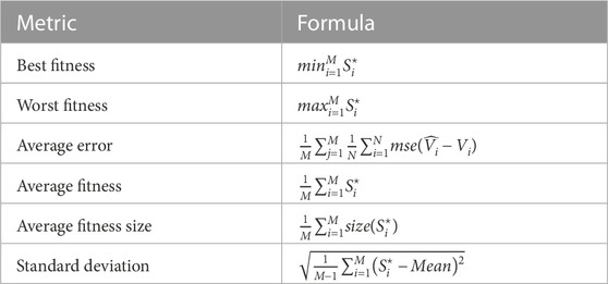
TABLE 3. The metrics used in evaluating the feature selection results.

TABLE 4

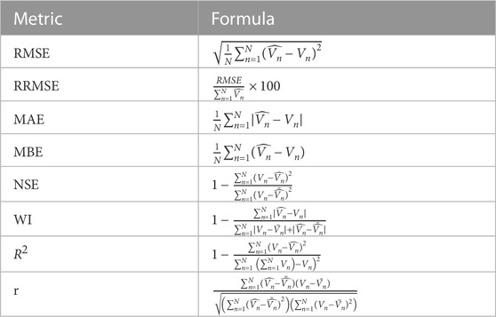
TABLE 4. The metrics used in evaluating the wind speed prediction results.

3.3 Feature selection results

The evaluation of the feature selection results are discussed in this section. Table 5 presents the results achieved by the proposed feature selection compared to other feature selection methods. In this table, the average error metric indicates the misclassification rate of the feature selection algorithm. In this case, the average error rate is 0.406, which suggests that the algorithm is correct about 59.4% of the time (since the error rate is 1 - accuracy). This metric can be useful in evaluating the overall performance of the feature selection algorithm. The average select size metric indicates the average percentage of the selected feature set. In this case, the average percentage is 0.379, which suggests that the algorithm selects fewer features when compared to the other methods in the table. This can indicate that the algorithm is effective at identifying a small subset of important predictors. The Average Fitness metric indicates the average fitness or quality of the selected feature set. Fitness measures how well the selected features predict the outcome variable (in this case, wind speed). In this case, the average fitness is 0.489, which suggests that the selected feature set performs reasonably well at predicting wind speed. The Best Fitness metric indicates the best fitness or quality of the selected feature set. In this case, the best fitness is 0.391, which suggests that the algorithm was able to identify a subset of features that performs well at predicting wind speed. The Worst Fitness metric indicates the worst fitness or quality of the selected feature set. In this case, the worst fitness is the same as the average fitness (0.489), which suggests that no selected feature sets perform significantly worse than average. The Std. The fitness metric indicates the fitness scores’ standard deviation for the selected feature sets. A larger standard deviation indicates that the fitness scores are more spread out, while a smaller standard deviation indicates that they are more tightly clustered. In this case, the standard deviation is 0.311, which suggests that the fitness scores are moderately spread out. These results suggest that the proposed feature selection algorithm (bGADTO) can identify a small subset of important predictors that perform reasonably well at predicting wind speed. While the average error rate of 0.406 suggests that the algorithm may not be highly accurate, the fact that the best fitness score is relatively low (0.391) suggests that there are selected feature sets that perform quite well. The moderate standard deviation of fitness scores suggests that the algorithm can identify multiple feature sets that perform reasonably well.

TABLE 5

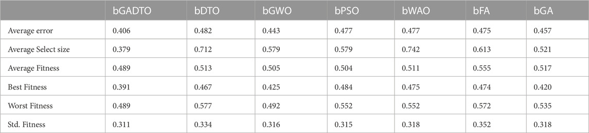
TABLE 5. Evaluation results of the proposed feature selection method and other methods.

On the other hand, the study of the statistical difference of the proposed feature selection algorithm compared to different algorithms is performed using the analysis of variance (ANOVA) test as shown in Table 6. In this table, [Treatment, SS] = 0.04658 represents the sum of squares for the treatment effect. It measures the variation in the response variable (e.g., wind speed) that is explained by the treatment (e.g., the feature selection algorithm). In this case, the sum of squares is 0.04658. [Treatment, DF] = 6 represents the degrees of freedom for the treatment effect. It is calculated as the number of treatments minus one. In this case, there are six treatments, so the degrees of freedom are six minus one or five. [Treatment, MS] = 0.007763: This represents the mean square for the treatment effect. It is calculated by dividing the sum of squares by the degrees of freedom. In this case, the mean square is 0.007763. [Treatment, F (6, 63)] = 144.8: This represents the F-statistic for the treatment effect. It is calculated by dividing the mean square for the treatment effect by the mean square for the error term (which measures the variation in the response variable that is not explained by the treatment). In this case, the F-statistic is 144.8. [Treatment, p-value] = “¡0.0001”: This represents the p-value for the treatment effect. It measures the probability of observing the F-statistic (or a more extreme F-statistic) if the null hypothesis is true (i.e., if the treatment does not affect the response variable). A p-value of less than 0.05 is typically considered statistically significant, which means we can reject the null hypothesis and conclude that the treatment significantly affects the response variable. These results suggest that the feature selection algorithm significantly affects the prediction of wind speed. The F-statistic of 144.8 and the p-value of less than 0.0001 indicate that the variation in wind speed explained by the feature selection algorithm is significantly greater than the variation not explained by the algorithm. The relatively large F-statistic and low p-value suggests that the effect of the feature selection algorithm is quite strong. The results also provide some information about the specific treatments that were used in the experiment. The fact that there are six degrees of freedom for the treatment effect suggests that there were six different treatments (e.g., six different feature selection algorithms or six different parameter settings for a single algorithm). The mean square for the treatment effect (0.007763) indicates that there is relatively little variation between the different treatments, while the sum of squares (0.04658) indicates that there is a significant amount of variation overall. This suggests that some treatments may be more effective than others but that no clear winner consistently outperforms the others. Overall, these ANOVA results provide valuable information about the effectiveness of a feature selection algorithm for wind speed prediction. They suggest that the algorithm significantly affects wind speed prediction and that there may be some variability in the performance of different treatments.

TABLE 6

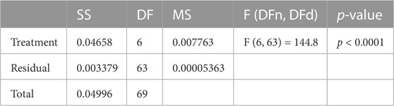
TABLE 6. ANOVA test applied to the feature selection evaluation results.

The Wilcoxon test results are shown in Table 7. The Wilcoxon signed-rank test is a non-parametric statistical test used to compare two related samples. In the context of feature selection for wind speed prediction, it can be used to determine whether a feature selection algorithm significantly improves the accuracy of the predictions. The theoretical median = 0 refers to the expected median of the distribution of the differences between the predicted wind speed values with and without the feature selection algorithm. A theoretical median of 0 suggests that there should be no significant difference between the two sets of predictions. The actual median = 0.406 refers to the observed median of the distribution of the differences between the predicted wind speed values with and without the feature selection algorithm. An actual median significantly different from the theoretical median suggests a significant difference between the two sets of predictions. The number of values = 10 refers to the number of paired observations used in the Wilcoxon signed-rank test. Each observation consists of the difference between the predicted wind speed values with and without the feature selection algorithm. Sum of signed ranks (W) = 55 refers to the sum of the signed ranks of the differences between the predicted wind speed values with and without the feature selection algorithm. The signed ranks are calculated by ranking the absolute values of the differences and then assigning positive or negative signs based on whether the original difference was positive or negative. A larger sum of signed ranks suggests a significant difference between the two sets of predictions. The sum of positive ranks = 55 refers to the sum of the ranks assigned to the positive differences between the predicted wind speed values with and without the feature selection algorithm. A larger sum of positive ranks suggests that the predictions with the feature selection algorithm are consistently better than those without the algorithm. The sum of negative ranks = 0 refers to the sum of the ranks assigned to the negative differences between the predicted wind speed values with and without the feature selection algorithm. A sum of negative ranks of 0 suggests that the predictions without the feature selection algorithm are not consistently better than the predictions with the algorithm. p-value = 0.002 refers to the probability of obtaining a test statistic as extreme as the observed one (i.e., a sum of signed ranks of 55) under the null hypothesis that there is no significant difference between the two sets of predictions. A p-value of less than 0.05 is typically considered statistically significant, which means we can reject the null hypothesis and conclude that the feature selection algorithm significantly improves the accuracy of the wind speed predictions. Discrepancy = 0.406 refers to the median difference between the predicted wind speed values with and without the feature selection algorithm. A larger discrepancy suggests that the predictions with the feature selection algorithm are consistently better than those without the algorithm. These Wilcoxon signed rank test results provide evidence that the feature selection algorithm significantly improves the accuracy of the wind speed predictions. The observed median of 0.406 and the p-value of 0.002 suggest that the difference between the predicted wind speed values with and without the feature selection algorithm is significant. The sum of signed ranks of 55 and positive ranks of 55 further support this conclusion, indicating that the predictions with the feature selection algorithm are consistently better than those without the algorithm. Overall, these results provide valuable insights into the effectiveness of the feature selection algorithm for wind speed prediction.

TABLE 7

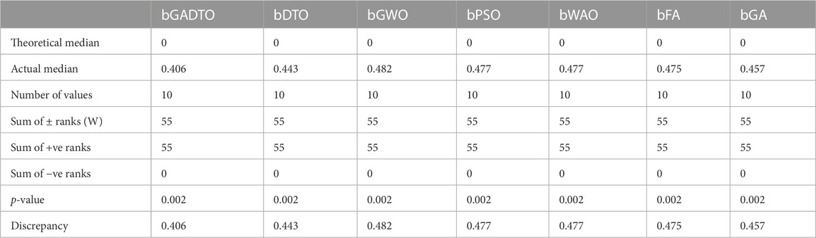
TABLE 7. Wilcoxon test applied to the RMSE results of feature selection methods.

Figure 8 shows the average error of the feature selection algorithms when compared with the proposed feature selection method. In this figure, the proposed method achieves the smallest average error, which indicates the superiority of the proposed method compared to the other six methods. In addition, several plots can be used to visualize the results of the ANOVA test, as shown in Figure 7. The residual, homoscedasticity, QQ, and heatmap plots are commonly used. The residual plot is a scatter plot of the predicted values versus the residuals (i.e., the differences between the actual and predicted values). A good residual plot should show no clear pattern, indicating that the model makes unbiased predictions. In the context of wind speed prediction, a residual plot can be used to evaluate the accuracy of a model’s predictions. The homoscedasticity plot is a scatter plot of the predicted values versus the residuals. The residuals are plotted on the y-axis, and the predicted values are on the x-axis. A good homoscedasticity plot should show no clear pattern, indicating that the variance of the residuals is constant across all predicted values. In wind speed prediction, a homoscedasticity plot can be used to evaluate the stability of a model’s predictions. The QQ plot is a scatter plot of the quantiles of the residuals versus the quantiles of a normal distribution. A good QQ plot should show the residuals following a straight line, indicating that they are normally distributed. In the context of wind speed prediction, a QQ plot can be used to evaluate the normality of the residuals. The heatmap plot is a visual representation of a matrix, where colors represent the values of the matrix. In wind speed prediction, a heatmap plot can be used to visualize the correlation between different features or models. By analyzing these plots, we can identify any patterns or outliers that may be affecting the accuracy of our wind speed prediction model. We can also use these plots to compare the accuracy of different models or feature selection methods. For example, suppose that one feature selection method consistently produces a lower residual variance than another. In that case, we can conclude that it is a better method for our wind speed prediction task.

FIGURE 7

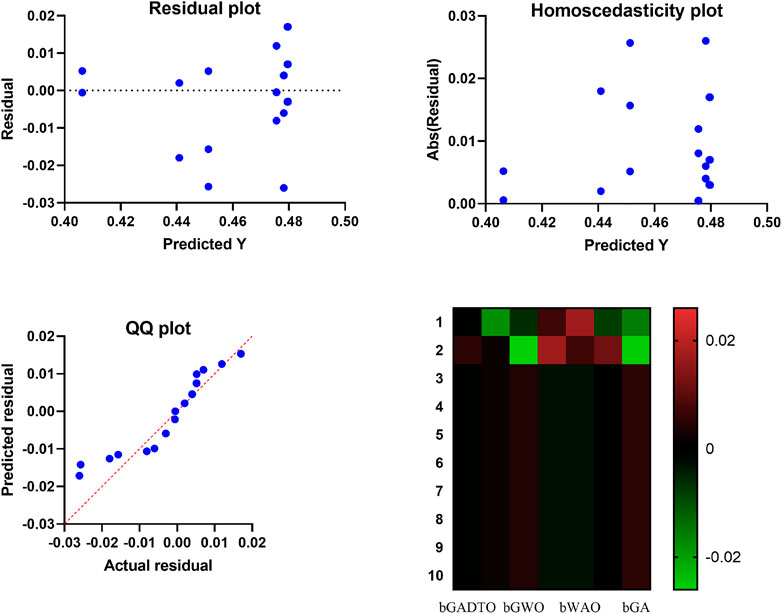
FIGURE 7. Analysis plots of the results achieved by the proposed feature selection algorithm.

FIGURE 8

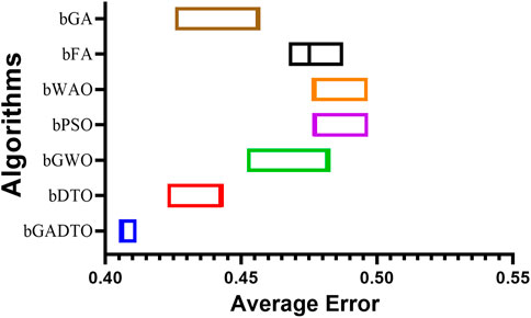
FIGURE 8. The average error of the results achieved by the proposed feature selection algorithm.

3.4 Wind speed forecasting results

The evaluation of the forecasting results of the wind speed using the baseline BiLSTM prediction model are shown in Table 8. In this table, the RMSE measures how far off the model’s predictions are from the true values, on average. An RMSE of 0.012 means that the average difference between the model’s predictions and the true values is 0.012 units of wind speed. This can be useful in assessing the overall accuracy of the model. MAE is another measure of the model’s prediction accuracy. It is similar to RMSE but looks at the absolute difference between the model’s predictions and the true values rather than the squared difference. An MAE of 0.007 means that, on average, the model’s predictions are off by 0.007 units of wind speed. MBE is also a measure of the overall bias in the model’s predictions. It tells us whether the model overestimates or underestimates the true values. In this case, an MBE of −0.001 means that, on average, the model’s predictions are lower than the true values. The r coefficient measures the linear relationship between the model’s predictions and the true values. A value of 0.998 suggests a strong positive linear relationship between the two, which is a good sign for the model’s predictive power. R² measures how much variation in the wind speed data can be explained by the model’s predictions. A value of 0.997 means that 99.7% of the variation in the data can be accounted for by the model, which is another indication that the model is performing well. The RRMSE is a normalized version of the RMSE that considers the range of the wind speed data. A value of 2.251 means that the RMSE is 2.251% of the range of the data, which can help to put the RMSE in context and compare it to other models. The NSE measures the model’s predictive efficiency relative to the mean of the observed data. A value of 0.997 suggests that the model performs nearly as well as the “perfect” model, which would have an NSE of 1. The WI is another measure of the model’s predictive efficiency. A value of 0.981 means that the model’s predictions are promising, with only 1.9% error compared to the average absolute error of the observations. Although these results are promising, but they still need more improvements to boost the prediction efficiency. This motivate the authors of this paper to develop new optimization algorithms to boost the performance of the BiLSTM prediction model to achieve more efficient results.

TABLE 8

TABLE 8. Results of evaluating wind speed forecasting using the baseline BiLSTM prediction model.

The statistical analysis of the results is shown in Table 9. Ten different scenarios were used to assess the accuracy of wind speed forecasts and generate these findings. The proposed approach (GADTO + BiLSTM) has this table’s lowest minimum and maximum error values. Furthermore, the skewness of a distribution of predicted wind speeds quantifies this asymmetry. The distribution is substantially skewed to the left (negatively skewed), skewness of −3.148. This indicates that it is more likely than not that the predicted wind speeds will be lower than the actual values. Kurtosis quantifies how “peaky” the distribution of predicted wind speeds is. With a kurtosis of 9.934, the distribution is likely to be highly peaked, with a more pronounced peak than in a normal distribution. This may suggest that the wind speed estimates are less dispersed around the mean. The harmonic mean is a special kind of average that differs from the more typical arithmetic mean in its calculation method. The average reciprocal of the predicted wind speeds is 0.00045, which gives us the harmonic mean of predicted wind speeds of 0.00045. Calculating average speeds over a specified period is one example of an application where this might be helpful. The median indicates the average value of a set of estimates for wind speed. Half of the estimates for the wind speed will be lower than the median of 0.00045, while the other half will be higher. This can be helpful when the predicted wind speed distribution has outliers that could throw off the average. Together, these measures of quality assurance point to a wind speed prediction distribution that is substantially skewed to the left and has a stronger peak than a normal distribution would. According to the harmonic mean and median, the average predicted wind speed is roughly 0.00045. With these measures, we may learn more about the dispersion and central tendency of the predicted wind speeds and how they compare to the actual values. These findings validate the proposed method’s advantage over four competing strategies. In addition, the RMSE results presents in this table significantly outperform the results achieved by the baseline BiLSTM, which proves the effectiveness of the proposed methodology.

TABLE 9

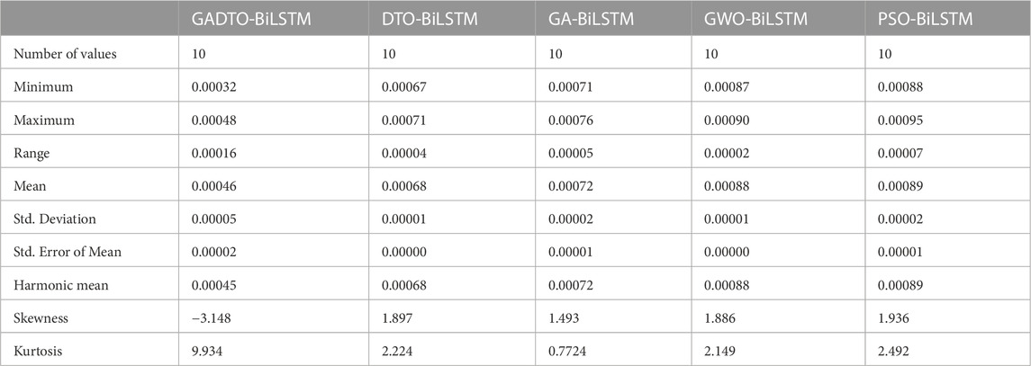
TABLE 9. Statistical analysis of the RMSE of the prediction results achieved using the proposed GADTO-BiLSTM compared to other methods.

The results of the ANOVA test, when applied to the results of the wind speed prediction using the optimized BiLSTM prediction model, are shown in Table 10. The F-statistic is a test statistic used to compare the degree to which one group (treatment) varies from another. Our F-statistic is a very respectable 420.8. Within-group degrees of freedom are indicated by the number (45), while between-group degrees of freedom is measured by the number (45). The number of groups or treatments and sample size determines the degrees of freedom. If the F-statistic is large, then the variability between groups is larger than the variability within groups. This p-value is related to the F-statistic (P0.0001). Under the assumption that the null hypothesis is correct, the p-value indicates the likelihood of witnessing the calculated test statistic (i.e., no differences between the groups). For statistical significance, the p-value must be less than 0.05, indicating substantial evidence against the null hypothesis. The p-value, in this case, is less than 0.0001, suggesting statistically significant variations in predicted wind speed across the treatment groups. Based on these findings, the predicted wind speeds vary significantly between the various groups or treatments. A high degree of variability between groups relative to within groups is shown by the F-statistic of 420.8 and the p-value of less than 0.0001, providing strong evidence against the null hypothesis that there are no differences between the groups.

TABLE 10

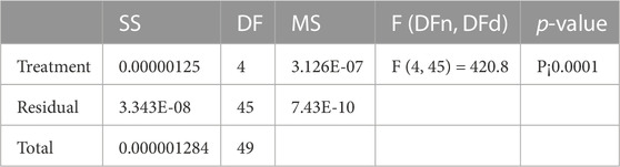
TABLE 10. ANOVA test results when applied to the wind speed predictions achieved by the proposed and the competing algorithms.

Table 11 presents the Wilcoxon signed rank test results. Similar to the ANOVA test, the Wilcoxon test is applied to the prediction results using the proposed optimized BiLSTM and the other optimization methods. The results in this table show the statistical difference between the proposed and other methods.

TABLE 11

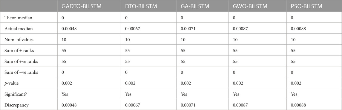
TABLE 11. Wilcoxon test results when applied to the wind speed predictions achieved by the proposed and the competing algorithms.

The RMSE values calculated for the achieved results of the proposed GADTO-BiLSTM method and other methods are shown in Figure 9. In this figure, the proposed method achieved the minimum value of RMSE, which emphasizes the superiority of the proposed method.

FIGURE 9

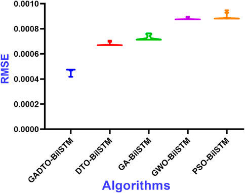
FIGURE 9. The RMSE values measured from the results achieved by the proposed and other compared optimization methods when applied to optimize the BiLSTM forecasting model.

This experiment helps study the stability of the proposed approach for various test cases. The histogram of the RMSE values is depicted in Figure 10. This histogram shows the number of experiments and the RMSE value achieved for each experiment. The figure shows that most test cases achieved the minimum RMSE values, reflecting the proposed method’s stability. In addition, the plots shown in Figure 11 are used to visualize the prediction results using the proposed GADTO-BiLSTM. The residual error shown in residual and homoscedasticity plots is minimal in these plots, emphasizing the robustness of the prediction results. In addition, the QQ plot and heatmap show accurate results and thus confirm the proposed methodology’s effectiveness.

FIGURE 10

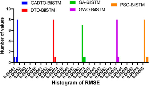
FIGURE 10. Histogram of the RMSE achieved by the proposed and other methods for optimization methods when applied to optimize the BiLSTM forecasting model.

FIGURE 11

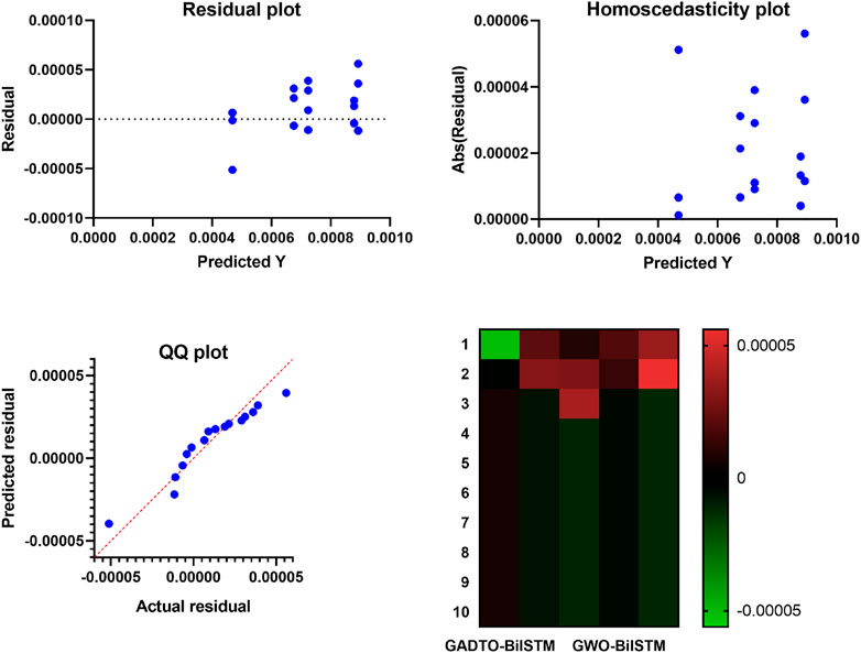
FIGURE 11. Visualizing the results of the achieved prediction results achieved by the optimized BiLSTM forecasting model.

3.5 Discussion

To robustly handle the wind speed forecasting process, we evaluated two algorithms in this section. The first algorithm was developed to optimize the BiLSTM prediction model to improve prediction results. Whereas the second algorithm was developed to address the feature selection process to guarantee to perform the prediction in terms of the best set of features. This algorithm proposed to fill the gap of low accuracy of the current prediction models. In this section, two sets of experiments were conducted. The first experiment targeted evaluating the performance of the proposed feature selection algorithm, bGADTO. To prove the effectiveness of the proposed algorithm, six recent feature selection algorithms were included in the conducted experiments. The results proved the superiority of the proposed methodology based on a standard set of evaluation criteria. On the other hand, the second set of experiments was conducted to evaluate the performance of the optimized BiLSTM model, which is optimized using the proposed GADTO algorithm. Four other approaches were employed in the conducted experiment to show the effectiveness and superiority of the proposed model. The presented results in this section and the visual plots confirmed the proposed methodology’s effectiveness and efficiency in predicting wind speed with the smallest error. The main advantage of this work is that the proposed optimization algorithm could improve the performance of the BiLSTM forecasting model as one of the most common approach in predicting time series data. The results showed that the improvements achieved by the proposed optimization algorithm are superior to the other optimization algorithms. The limitations of this algorithm are not clearly identified in this work, but it is planned to use this algorithm, in the future work, with more prediction tasks of varying sizes to identify its limitations.

4 Conclusion

One of the essential factors in the efficient distribution of electricity is the quality of the energy management system, which has been the focus of recent studies in the field of renewable energy. Predicting how fast the wind will blow is another crucial factor. This paper proposes a new approach for robust wind speed prediction based on BiLSTM and a novel optimization algorithm. The proposed optimization algorithm is based on GA and DTO and is referred to as the GADTO algorithm. This optimization algorithm is used to optimize the parameters of BiLSTM prediction model. GADTO-BiLSTM denotes the optimized model. In addition, the binary version of this optimization algorithm is used for selecting the most significant set of features to boost the prediction accuracy. To prove the superiority of the proposed method, four other optimization methods are included in the conducted experiments. The proposed approach is evaluated in terms of a freely available Kaggle dataset used as the benchmark dataset. The results of the proposed feature selection method and the proposed optimized model are evaluated using a set of criteria and statistical tests compared to other competing methods. These tests’ results emphasized the proposed method’s statistical difference and superiority in predicting wind speed in the adopted dataset. Based on the adopted evaluation criteria, the achieved RMSE is (0.012), MAE is (0.007), MBE is (−0.001), r is (0.998), R² is (2.251), NSE is (0.997), and WI is (0.981). These results confirm the effectiveness of the proposed methodology in wind speed prediction. The future perspective of this work includes evaluating the proposed methodology on a larger dataset and including more optimization methods and prediction models to confirm the superiority of the proposed methodology.

Data availability statement

The original contributions presented in the study are included in the article/supplementary material, further inquiries can be directed to the corresponding author.

Author contributions

Conceptualization, ME; methodology, AA and E-SE-K; software, E-SE-K and ME; validation, DK; formal analysis, AA and DK; investigation, E-SE-K and ME; writing—original draft, ME, AA, AI, and DK; writing—review & editing, AA, AI, and E-SE-K; visualization, AA and AI; project administration, E-SE-K, and All authors contributed to the article and approved the submitted version.

Funding

Princess Nourah bint Abdulrahman University Researchers Supporting Project number (PNURSP 2023R 308), Princess Nourah bint Abdulrahman University, Riyadh, Saudi Arabia.

Conflict of interest

The authors declare that the research was conducted in the absence of any commercial or financial relationships that could be construed as a potential conflict of interest.

Publisher’s note

All claims expressed in this article are solely those of the authors and do not necessarily represent those of their affiliated organizations, or those of the publisher, the editors and the reviewers. Any product that may be evaluated in this article, or claim that may be made by its manufacturer, is not guaranteed or endorsed by the publisher.

References

Abdel Samee, N., El-Kenawy, M., Atteia, G., Jamjoom, M., Ibrahim, A., Abdelhamid, A., et al. (2022). Metaheuristic optimization through deep learning classification of COVID-19 in chest X-ray images. Comput. Mater. Continua73, 4193–4210.

CrossRef Full Text | Google Scholar

Akhil, V., Wadhvani, R., Gyanchandani, M., and Kushwah, A. K. (2022). “Clustering-based hybrid approach for wind speed forecasting,” in Proceedings of data analytics and management Editors D. Gupta, Z. Polkowski, A. Khanna, S. Bhattacharyya, and O. Castillo (Singapore: Springer Nature), 587–598. doi:10.1007/978-981-16-6289-8_49

CrossRef Full Text | Google Scholar

Albalawi, H., El-Shimy, M. E., AbdelMeguid, H., Kassem, A. M., and Zaid, S. A. (2022). Analysis of a hybrid wind/photovoltaic energy system controlled by brain emotional learning-based intelligent controller. Sustainability14, 4775. doi:10.3390/su14084775

CrossRef Full Text | Google Scholar

Ariyaratne, M., and Fernando, T. (2023). A comprehensive review of the firefly algorithms for data clustering. Cham: Springer International Publishing, 217. doi:10.1007/978-3-031-09835-2_12

CrossRef Full Text | Google Scholar

Awange, J. L., Paláncz, B., Lewis, R. H., and Völgyesi, L. (2018). “Particle swarm optimization,” in Mathematical geosciences: Hybrid symbolic-numeric methods Editors J. L. Awange, B. Paláncz, R. H. Lewis, and L. Völgyesi (Cham: Springer International Publishing). 167–184. doi:10.1007/978-3-319-67371-4_6

CrossRef Full Text | Google Scholar

Brown, B. G., Katz, R. W., and Murphy, A. H. (1984). Time series models to simulate and forecast wind speed and wind power. J. Appl. Meteorology Climatol.23, 1184–1195. doi:10.1175/1520-0450(1984)023⟨1184:TSMTSA-2.0.CO;2

CrossRef Full Text | Google Scholar

Cadenas, E., Rivera, W., Campos-Amezcua, R., and Heard, C. (2016). Wind speed prediction using a univariate ARIMA model and a multivariate NARX model. Energies9, 109. doi:10.3390/en9020109

CrossRef Full Text | Google Scholar

Cadenas, E., and Rivera, W. (2009). Short term wind speed forecasting in La Venta, Oaxaca, México, using artificial neural networks. Renew. Energy34, 274–278. doi:10.1016/j.renene.2008.03.014

CrossRef Full Text | Google Scholar

Carvalho, D., Rocha, A., Gómez-Gesteira, M., and Santos, C. (2012). A sensitivity study of the WRF model in wind simulation for an area of high wind energy. Environ. Model. Softw.33, 23–34. doi:10.1016/j.envsoft.2012.01.019

CrossRef Full Text | Google Scholar

Chen, G., Tang, B., Zeng, X., Zhou, P., Kang, P., and Long, H. (2022). Short-term wind speed forecasting based on long short-term memory and improved BP neural network. Int. J. Electr. Power & Energy Syst.134, 107365. doi:10.1016/j.ijepes.2021.107365

CrossRef Full Text | Google Scholar

Demolli, H., Dokuz, A. S., Ecemis, A., and Gokcek, M. (2019). Wind power forecasting based on daily wind speed data using machine learning algorithms. Energy Convers. Manag.198, 111823. doi:10.1016/j.enconman.2019.111823

CrossRef Full Text | Google Scholar

Doaa, D. S., Karim, F. K., Alshetewi, S., Ibrahim, A., Abdelhamid, A. A., and El-kenawy, E. M. (2022). Optimized weighted ensemble using dipper throated optimization algorithm in metamaterial antenna. Comput. Mater. Continua73, 5771–5788. doi:10.32604/cmc.2022.032229

CrossRef Full Text | Google Scholar

Dumitru, C.-D., and Gligor, A. (2017). Daily average wind energy forecasting using artificial neural networks. Procedia Eng.181, 829–836. doi:10.1016/j.proeng.2017.02.474

CrossRef Full Text | Google Scholar

El-kenawy, E.-S. M., Albalawi, F., Ward, S. A., Ghoneim, S. S. M., Eid, M. M., Abdelhamid, A. A., et al. (2022a). Feature selection and classification of transformer faults based on novel meta-heuristic algorithm. Mathematics10. doi:10.3390/math10173144

CrossRef Full Text | Google Scholar

El-Kenawy, E.-S. M., Mirjalili, S., Abdelhamid, A. A., Ibrahim, A., Khodadadi, N., and Eid, M. M. (2022b). Meta-heuristic optimization and keystroke dynamics for authentication of smartphone users. Mathematics10. doi:10.3390/math10162912

CrossRef Full Text | Google Scholar

Eldali, F. A., Hansen, T. M., Suryanarayanan, S., and Chong, E. K. P. (2016). “Employing ARIMA models to improve wind power forecasts: A case study in ercot,” in 2016 North American Power Symposium (NAPS), Denver, CO, USA, 18-20 September 2016. doi:10.1109/NAPS.2016.7747861

CrossRef Full Text | Google Scholar

Fang, S., and Chiang, H. (2016). Improving supervised wind power forecasting models using extended numerical weather variables and unlabelled data. IET Renew. Power Gener.10, 1616–1624. doi:10.1049/iet-rpg.2016.0339

CrossRef Full Text | Google Scholar

Fathima, A. H., and Palanisamy, K. (2016). Energy storage systems for energy management of renewables in distributed generation systems. London, UK: IntechOpen. doi:10.5772/62766

CrossRef Full Text | Google Scholar

Fedesoriano, F. (2022). Wind speed prediction dataset. [Online] Available at: https://www.kaggle.com/datasets/fedesoriano/wind-speed-prediction-dataset. [Accessed 2023 01 01]

Google Scholar

Higashiyama, K., Fujimoto, Y., and Hayashi, Y. (2017). “Feature extraction of numerical weather prediction results toward reliable wind power prediction,” in 2017 IEEE PES Innovative Smart Grid Technologies Conference Europe (ISGT-Europe), Torino, Italy, September 26-29, 2017. doi:10.1109/ISGTEurope.2017.8260216

CrossRef Full Text | Google Scholar

Hoolohan, V., Tomlin, A. S., and Cockerill, T. (2018). Improved near surface wind speed predictions using Gaussian process regression combined with numerical weather predictions and observed meteorological data. Renew. Energy126, 1043–1054. doi:10.1016/j.renene.2018.04.019

CrossRef Full Text | Google Scholar

Immanuel, S. D., and Chakraborty, U. K. (2019). “Genetic algorithm: An approach on optimization,” in 2019 International Conference on Communication and Electronics Systems (ICCES), July 17-19,2019, 701. doi:10.1109/ICCES45898.2019.9002372

CrossRef Full Text | Google Scholar

Kavasseri, R. G., and Seetharaman, K. (2009). Day-ahead wind speed forecasting using f-ARIMA models. Renew. Energy34, 1388–1393. doi:10.1016/j.renene.2008.09.006

CrossRef Full Text | Google Scholar

Khafaga, D. S., Alhussan, A. A., El-Kenawy, E.-S. M., Ibrahim, A., Eid, M. M., and Abdelhamid, A. A. (2022). Solving optimization problems of metamaterial and double t-shape antennas using advanced meta-heuristics algorithms. IEEE Access10, 74449–74471. doi:10.1109/ACCESS.2022.3190508

CrossRef Full Text | Google Scholar

Li, C., Lin, S., Xu, F., Liu, D., and Liu, J. (2018). Short-term wind power prediction based on data mining technology and improved support vector machine method: A case study in northwest China. J. Clean. Prod.205, 909–922. doi:10.1016/j.jclepro.2018.09.143

CrossRef Full Text | Google Scholar

Liu, H., Mi, X., and Li, Y. (2018). Smart deep learning based wind speed prediction model using wavelet packet decomposition, convolutional neural network and convolutional long short term memory network. Energy Convers. Manag.166, 120–131. doi:10.1016/j.enconman.2018.04.021

CrossRef Full Text | Google Scholar

Liu, X., Lin, Z., and Feng, Z. (2021). Short-term offshore wind speed forecast by seasonal ARIMA - a comparison against GRU and LSTM. Energy227, 120492. doi:10.1016/j.energy.2021.120492

CrossRef Full Text | Google Scholar

López, G., and Arboleya, P. (2022). Short-term wind speed forecasting over complex terrain using linear regression models and multivariable LSTM and NARX networks in the Andes Mountains, Ecuador. Renew. Energy183, 351–368. doi:10.1016/j.renene.2021.10.070

CrossRef Full Text | Google Scholar

Mirjalili, S., and Lewis, A. (2016). The whale optimization algorithm. Adv. Eng. Softw.95, 51–67. doi:10.1016/j.advengsoft.2016.01.008

CrossRef Full Text | Google Scholar

Mirjalili, S., Mirjalili, S. M., and Lewis, A. (2014). Grey wolf optimizer. Adv. Eng. Softw.69, 46–61. doi:10.1016/j.advengsoft.2013.12.007

CrossRef Full Text | Google Scholar

Praveena, R., and Dhanalakshmi, K. (2018). “Wind power forecasting in short-term using Fuzzy K-means clustering and neural network,” in 2018 International Conference on Intelligent Computing and Communication for Smart World (I2C2SW), Erode, India, 14th to 15th December 2018, 336–339. doi:10.1109/I2C2SW45816.2018.8997350

CrossRef Full Text | Google Scholar

Rajagopalan, S., and Santoso, S. (2009). “Wind power forecasting and error analysis using the autoregressive moving average modeling,” in 2009 IEEE Power & Energy Society General Meeting, Calgary, Alberta, Canada, 26-30 July 2009, 1. doi:10.1109/PES.2009.5276019

CrossRef Full Text | Google Scholar

Saeed, A., Li, C., Danish, M., Rubaiee, S., Tang, G., Gan, Z., et al. (2020). Hybrid bidirectional LSTM model for short-term wind speed interval prediction. IEEE Access8, 182283–182294. doi:10.1109/ACCESS.2020.3027977

CrossRef Full Text | Google Scholar

Sami Khafaga, D., Ali Alhussan, A., El-kenawy, M., Ibrahim, A., Abd Elkhalik, H., El-Mashad, Y. S., et al. (2022). Improved prediction of metamaterial antenna bandwidth using adaptive optimization of LSTM. Comput. Mater. Continua73, 865–881.

CrossRef Full Text | Google Scholar

Sami Khafaga, D., Ali Alhussan, A., El-kenawy, M., Takieldeen, E., Hassan, A. ., M., Hegazy, T., et al. (2022). Meta-heuristics for feature selection and classification in diagnostic breast-cancer. Comput. Mater. Continua73, 749–765.

CrossRef Full Text | Google Scholar

Sfetsos, A. (2002). A novel approach for the forecasting of mean hourly wind speed time series. Renew. Energy27, 163–174. doi:10.1016/S0960-1481(01)00193-8

CrossRef Full Text | Google Scholar

Shabbir, N., Kt, L., Jawad, M., Husev, O., Ur Rehman, A., Abid Gardezi, A., et al. (2022). Short-term wind energy forecasting using deep learning-based predictive analytics. Comput. Mater. Continua72, 1017–1033. doi:10.32604/cmc.2022.024576

CrossRef Full Text | Google Scholar

Shang, Z., He, Z., Chen, Y., Chen, Y., and Xu, M. (2022). Short-term wind speed forecasting system based on multivariate time series and multi-objective optimization. Energy238, 122024. doi:10.1016/j.energy.2021.122024

CrossRef Full Text | Google Scholar

Sun, F., and Jin, T. (2022). A hybrid approach to multi-step, short-term wind speed forecasting using correlated features. Renew. Energy186, 742–754. doi:10.1016/j.renene.2022.01.041

CrossRef Full Text | Google Scholar

Takieldeen, E., El-kenawy, A. ., M., Hadwan, M., and Zaki, M. R. (2022). Dipper throated optimization algorithm for unconstrained function and feature selection. Comput. Mater. Continua72, 1465–1481. doi:10.32604/cmc.2022.026026

CrossRef Full Text | Google Scholar

Torres, J. L., García, A., De Blas, M., and De Francisco, A. (2005). Forecast of hourly average wind speed with ARMA models in Navarre (Spain). Sol. Energy79, 65–77. doi:10.1016/j.solener.2004.09.013

CrossRef Full Text | Google Scholar

Xiong, B., Lou, L., Meng, X., Wang, X., Ma, H., and Wang, Z. (2022). Short-term wind power forecasting based on attention mechanism and deep learning. Electr. Power Syst. Res.206, 107776. doi:10.1016/j.epsr.2022.107776

CrossRef Full Text | Google Scholar

Yu, C., Li, Y., Bao, Y., Tang, H., and Zhai, G. (2018). A novel framework for wind speed prediction based on recurrent neural networks and support vector machine. Energy Convers. Manag.178, 137–145. doi:10.1016/j.enconman.2018.10.008

CrossRef Full Text | Google Scholar

Yu, R., Liu, Z., Li, X., Lu, W., Ma, D., Yu, M., et al. (2019). Scene learning: Deep convolutional networks for wind power prediction by embedding turbines into grid space. Appl. Energy238, 249–257. doi:10.1016/j.apenergy.2019.01.010

CrossRef Full Text | Google Scholar

Zeng, P., Sun, X., and Farnham, D. J. (2020). Skillful statistical models to predict seasonal wind speed and solar radiation in a Yangtze River estuary case study. Sci. Rep.10, 8597. doi:10.1038/s41598-020-65281-w

PubMed Abstract | CrossRef Full Text | Google Scholar