Optimized ensemble model for wind power forecasting using hybrid whale and dipper-throated optimization algorithms

1 Introduction

Economic and social progress is aided by energy extraction and use (Zhang et al., 2020). Rapid industrialization and population increase have made the world more concerned about the energy dilemma in recent years (Li et al., 2020). Sustainable economic growth and social stability are hampered (Kong et al., 2020) by the world’s energy crisis and environmental degradation. As a result, future development should center on boosting the transition from clean energy and constructing a low-carbon and environmentally friendly renewable energy system and traditional fossil fuels to green. Nations worldwide are issuing laws encouraging sustainable energy research, development, and deployment. Wind power is the second most popular renewable energy source (Kusiak et al., 2013) because it is clean and produces no pollution. As a prototype of renewable energy generation technology, wind power generation has received much attention and development. It is now commonly seen as a viable alternative to the more conventional thermal method of producing electricity. The following are the primary benefits compared to other electricity production methods. Wind power is a sustainable and renewable resource. Second, because of its compact size and ease of use, generating wind power is a more practical option. There are other financial benefits to using this renewable energy source, as well (El-Kenawy et al., 2022a; Ariyaratne and Fernando, 2023). In conclusion, wind power has several positive attributes that make it ideal for commercial use, future expansion, and widespread application. A viable strategy for addressing both the worldwide energy issue and the greenhouse impact may be found in the advancement of wind power production technologies (Kisvari et al., 2021; Neshat et al., 2021; El-Kenawy et al., 2022b).

Wind power has numerous positive applications but is vulnerable to weather, geographical, and seasonal changes that might disrupt production. Due to the unpredictability of wind resources, wind turbine output is also highly intermittent and volatile (Majidi Nezhad et al., 2020), which can cause problems in a power grid’s scheduling, building, and operation. Although the steadily expanding wind power installed capacity contributes to an increase in the wind power scale connected to the grid (Abdelbaky et al., 2020), the aforementioned uncertainties will cause challenges in power quality, grid stability, dispatching, and operation of the power system in addition to the significant impact on the grid-connected wind power (Xu et al., 2021; Kong et al., 2022). Regulation of the time series energy distribution is crucial to ensuring a reliable power grid function. However, the non-linear nature of wind power makes this difficult to achieve. To address this issue, researchers need to figure out how to make the unpredictable character of the wind power supply predictable and how to anticipate wind power efficiently and reliably. These can decrease the impact on the power system while adding wind power to the grid. They may provide a solid theoretical basis and technological support for optimizing operation in the future and grid dispatching and security (Tian, 2020; Peng et al., 2021). Therefore, research into effective prediction approaches for wind power within the evolution of power systems is necessary due to wind power’s unpredictability. This study’s significance lies in the fact that it facilitates the development of renewable energy technologies; it opens the door to carbon-free, green, and environmentally friendly power generation methods; and ensures the smooth dispatch and operation of cutting-edge power grids (Tian and Wang, 2022; Yang et al., 2022).

This paper has made significant progress in wind power prediction due to the optimized ensemble model consisting of LSTM, BiLSTM, and GRU and the dynamic whale dipper-throated optimization (DWDTO) method. Wind power, for example, is becoming significant as a renewable energy source for meeting global energy demands and lowering carbon emissions. The optimal integration of wind energy into the grid, stable grid operation, and effective energy management depends on accurate wind power forecasts. The ensemble model draws on the advantages of three popular and effective deep-learning architectures for sequence modeling and prediction: LSTM, BiLSTM, and GRU. Modeling temporal trends in wind power data is made possible by LSTM (Long Short-Term Memory) networks’ ability to capture long-range relationships accurately. In contrast, BiLSTM (Bidirectional LSTM) networks process data in both directions, enabling them to record historical and prospective time-related contexts. GRU (Gated Recurrent Unit) networks effectively simplify LSTM, achieving similar performance with less computing overhead. The suggested DWDTO method is used to enhance the efficiency of the ensemble model. The DWDTO algorithm integrates ideas from both the WOA and the DTO, incorporating dynamic tactics to improve exploration and exploitation further. The DWDTO technique enhances convergence speed and guarantees resilient optimization of the ensemble model by adaptively modifying the algorithm’s parameters based on the current optimization progress. Experimental evidence shows that the suggested model performs better than standard optimization methods and standalone LSTM, BiLSTM, and GRU models. The DWDTO technique allows for efficient parameter optimization and the collaborative learning of several designs, which contribute to the performance boost. Accurate and trustworthy wind power predictions are made possible by the ensemble model’s successful capture of complex patterns and relationships in wind power data. This improved ensemble model has far-reaching consequences. It can improve energy management, grid stability, and cost-effectiveness by aiding in the operation and planning of wind power-producing systems. Reducing dependency on fossil fuels and fostering sustainable development, precise wind power forecasting also helps integrate renewable energy sources into existing power networks.

The paper is organized into six sections, beginning with an introduction. The literature review is then presented in Section 2. In Section 3, we analyze the proposed model’s performance metrics and examine the model’s thorough design approach. Section 4 begins with an overview of the dataset used in this paper, followed by an examination of the statistical tests run on the data to determine its internal features, then a discussion of how those features informed the selection of the model’s input variables and the initialization of its basic parameters, and finally a comparison of performance indicators of various methods and their measured results to illustrate the DWDTO model’s efficacy. Section 5 goes into further depth on the conclusion and what comes next.

2 Literature review

The methodologies and models used to predict the output of wind turbines have been the subject of study by researchers in recent years. These approaches may be generally divided into the four groups indicated in Figure 1, according to the criteria used to classify them (Wang et al., 2021). Depending on the underlying modeling theory, wind power prediction models may be broken down into the figure’s physical, statistical, and combination prediction models. Time series approaches, including kernel extreme learning machine (KELM), least squares support vector machine (LSSVM), autoregressive integrated moving average (ARIMA), Kalman filter, and Fractional-ARIMA (F-ARIMA), are among the most used statistical models for process prediction. Recently, deep neural networks (DNNs) such as long short-term memory (LSTM), auto-encoder (AE), and gated recurrent unit (GRU) have been widely employed in wind power prediction due to their superiority in dealing with non-linear issues and the ongoing development of deep learning techniques. Compared to the performance of conventional statistical and physical models, their ability to make accurate predictions has been vastly enhanced.

FIGURE 1

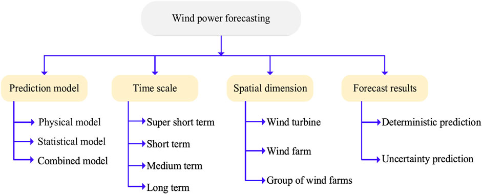
FIGURE 1. The various methods used in wind power forecasting.

With their increased proficiency in non-linear processing and the capacity to overcome the gradient disappearance problem during learning, LSTM networks have become increasingly popular for application in real-time predictive control of complex dynamic situations. The raw data on wind power generation was applied to LSTM, with the prediction error tuned using a Beta distribution, as in (Shahid et al., 2021). Using operational data from real-world wind farms, we created a unique LSTM-based model for forecasting wind power. Then we tuned the model’s hyperparameters to reduce the prediction error (Kong et al., 2020; Alhussan et al., 2022). Using LSTM and variational mode decomposition (VMD) to dissect and reassemble the raw power data, a more accurate short-term wind power prediction method was presented (Duan et al., 2021a). The LSTM is paired with a self-attentional temporal convolutional network to add an attentional mechanism. The proposed approach demonstrates the greatly enhanced forecast accuracy (Xiang et al., 2022) by comparing the data of several wind farms. Using a combination of convolutional neural networks (CNNs) and long short-term memory (LSTMs) with fine-tuned parameters, the power output of offshore wind turbines may be accurately forecasted. Reduced computation time and enhanced prediction accuracy resulted from optimizing the LSTM with adaptive differential evolution and the sines and cosines selection approach (Khan et al., 2021; Khafaga et al., 2022).

Despite LSTM’s impressive performance in time series prediction, it is relatively uncommon for the optimal global solution to be obscured by the seemingly trivial task of establishing network parameters during model training. Consequently, methods for optimizing parameters have been a topic of study (Memarzadeh and Keynia, 2020). The sparrow search algorithm (hence referred to as SSA or sparrow algorithm) is a revolutionary population intelligence optimization technique jointly proposed in 2020 (Xue and Shen, 2020). It is one of several new metaheuristic algorithms that have emerged as machine learning parameter optimization leaders. To find the best solution to the objective function (Kumar Ganti et al., 2022), we may model the actions of a flock of sparrows as they search for food and avoid predators. Using SSA optimization to set up network parameters boosts accuracy in comparison to other models [(Zhang and Ding, 2021), (Tian and Chen, 2021)]. For instance, SSA is employed in estimating ultra-short-term wind power to improve the input weight and other parameters of DELM (An et al., 2021). Short-term wind speed prediction was developed using LSTM and BPNN, and SSA was used to optimize the prediction model for varying degrees of complexity in the input sequence (Chen et al., 2022).

The model still has problems, such as delayed convergence with low accuracy (Liu G. et al., 2021). However, the enhancements above that let SSA leap out of a local optimum as often as possible during training to increase its search capabilities correspondingly. By studying how individual sparrows in the SSA do their iterative search, we can see how the quality of the population as a whole and the position update parameters significantly impact the algorithm’s capacity to identify an optimal (Venkata Rao and Venkata Rao, 2019; Zhang et al., 2021). When stuck in a local optimum, it might be difficult to escape the current region rapidly due to the iterative process’s absence of a variation mechanism (Li et al., 2022). After identifying these problems with the original SSA method, we build the DWDTO algorithm by introducing a Tent chaotic sequence and a Gaussian mutation technique to fix its flaws. A tent-chaotic sequence of births achieves a more diverse and high-quality beginning population (Tian and Wang, 2022). The algorithm’s stability and capacity for a global search are enhanced by using a Gaussian mutation technique (Alhussan et al., 2022; Yang et al., 2022).

Therefore, the research gap of the work presented in the literature is the lack of a robust and stable model that can perform wind power prediction efficiently. In this research, we proposed a novel approach for filling this gap regarding a new optimization algorithm and a new ensemble model. The proposed optimization algorithm is used in feature selection and optimizing the ensemble model’s parameters. This methodology can be used in applications based on predicting time series data. The following points summarize the novelty of this work.

• A new weighted ensemble model is proposed as an autonomous learning prediction model to address the multivariate non-linearity of wind farms.

• A new optimization algorithm is proposed based on a hybrid of whale optimization algorithm and dipper-throated algorithm to optimize the weights of the ensemble model.

• The binary version of the proposed optimization algorithm is utilized to select the significant features of the employed dataset.

• A set of statistical tests is performed to assess the superiority ans statistical difference of the proposed methodology.

3 The proposed methodology

The proposed methodology is based on a new optimization algorithm developed to optimize the weights of an ensemble composed of three prediction models namely, LSTM, BiLSTM and GRU. The block diagram of the proposed methodology is shown in Figure 2 and the structure of the prediction models is shown in Figure 3. This part begins with a comprehensive breakdown of the proposed model's specialized technique, followed by an explanation of the thinking behind the strategy used to merge the models.

FIGURE 2

FIGURE 2. The structure of the proposed methodology.

FIGURE 3

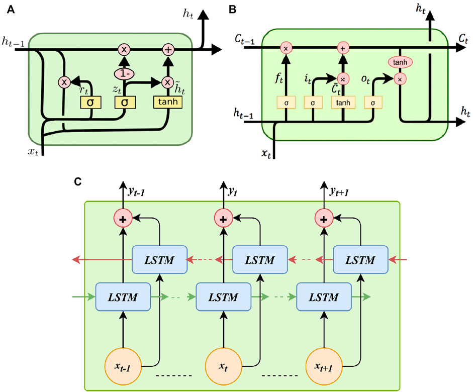
FIGURE 3. The prediction models included in the proposed ensemble model. (A) Gated recurrent unit (GRU), (B) Long short-time memory (LSTM), and (C) Bidirectional LSTM (BiLSTM).

3.1 Long short-term memory

As a subset of recurrent neural networks, long short-term memory (LSTM) networks can store large amounts of data in a relatively short amount of time (Kisvari et al., 2021; Ewees et al., 2022). As a result, the operation structure is changed, and the layer count of the original neural network is expanded from 1 to 4. Primarily, it is distinguished by its capacity for long-term data storage through encoding information in a conventional memory module. The network design implements the gate mechanism using the input, output, and forgetting gates of the algorithm nodes (Zhang et al., 2019). By randomly shuffling the weight coefficients of the connections in the appropriate ring, we can prevent gradient disappearance (Demolli et al., 2019; El-Kenawy et al., 2022a). It has seen widespread application in recent years for predicting renewable energy sources.

In contrast to traditional RNNs, LSTMs do not suffer from the long-term perception loss that happens when gradients diminish during training, making them ideally suited for constructing prediction models for wind turbine power generation. The forgetting gate, denoted by F_t, is formulated using the following equation (Liu M.-D. et al., 2021).

$F_t=\sigma \left(W_F{X}_t+U_F{h}_{t-1}+b_F\right)(1)$

Layer input is denoted by X_t in this context. The activation function, the bias term of the input layer b_F, the output layer weight W_F, and the hidden layer weight U_F all contribute to the final output, Ht − 1, which reflects the output of the preceding hidden layer. The activation function in this investigation is the ReLU function (Akhter et al., 2022), which is found using the formula:

$\sigma \left(x\right)=\mathit{max}\left(0,x\right)(2)$

There is a correlation between the forgetting gate’s value and the amount of history preserved at a certain site. The input gate, denoted by I_t, is the second gate shown (Ewees et al., 2022). It is obtained from the following equation.

$I_t=\sigma \left(W_I{X}_t+U_I{h}_{t-1}+b_I\right)(3)$

The following equation provides a method for obtaining the C_t gives (Liu et al., 2020). By multiplying the input gate’s data by the data at the other nodes, the LSTM can keep its information up to date. The value of the node is removed if the result is zero, but it is retained if the result is one.

${\widehat{C}}_t=\mathit{tanh}\left(W_C{X}_t+U_C{h}_{t-1}+b_C\right)(4)$

Figure 3 indicates, using the following equation, that a change must be made to the cell’s state (Zhang et al., 2021).

$C_t=F_t{C}_{t-1}+I_t{\widehat{C}}_t(5)$

O_t denotes the output gate, and the output value of the LSTM cell is calculated by multiplying its output value by its dynamic range value, where the following equations represent O_t and h_t (Qing and Niu, 2018).

$O_t=\sigma \left(W_O{X}_t+U_O{h}_{t-1}+b_O\right)(6)$

$h_t=O_t\mathit{tanh}\left(C_t\right)(7)$

With only two gates and a few more fixed parameters, GRU is a reduced variant of LSTM. In time series applications like machine translation and voice signal modeling, LSTM and GRU perform similarly. But since LSTM networks can handle bigger datasets (Xue and Shen, 2020), they are favored in this research over GRU.

For more precise predictions, researchers have developed bidirectional LSTMs, an enhanced variant of standard LSTMs that considers both past and future states. While traditional LSTMs only look at the past, Bidirectional LSTMs consider both the present and the future. Therefore, unlike regular LSTMs, which only process information in one way, BiDLSTMs process data in both the forward and backward directions. Figure 5 depicts the structure of a two-hidden-layer, bidirectional LSTM network. In BiDLSTM, two LSTM networks are trained: one processes the input sequence forwards, while the other does it backward using a mirror image of the original. At each iteration, the results from a pair of networks’ forward and backward layers are combined. So, BiDLSTM networks have superior learning performance.

3.2 Whale optimization algorithm

The whale optimization algorithm (WOA) is the bubble-net feeding algorithm. The activities of humpback whales inspire it during hunting and foraging and is one of the most recent heuristic optimization approaches described by authors in (Mirjalili and Lewis, 2016). This strategy has two primary phases: upward spirals and double loops. The whale dives at a depth of 12 m or less before beginning the upward spiral phase, during which it spirals around the prey, creating bubbles and swimming upstream. Second, the coral circulation is part of the double circulation phase, which involves the tail leaf fluttering the water surface and capturing the cycle. The foraging strategy involves producing unique bubbles in a cyclical or “9-shaped” motion. Only humpback whales are vulnerable to the unique bubble net predation.

There are not many moving parts or settings to tweak with the foraging approach. In the iterative process, humpback whales can escape the local optimum. The current best candidate result is also thought to be somewhat near to the intended quarry. If the best search agent is provided, the other agents will use that information to update their positions. The procedure for recalculating coordinates is explained as follows:

This is the global ideal outcome of the optimization problem and the location of the i-th whale in d-dimensional space relative to the d-th whale’s prey. Although humpback whales are adept at pinpointing the general area where their prey is hiding and then closing in on it, the exact location of the prey they are after is sometimes difficult to ascertain. After t iterations, WOA saves the target prey’s position as $X_t^{*}(X_t^1,X_t^2,\dots ,X_t^d)*$, where X is the number of other people within a given distance from the humpback whale. To calculate its current location, use the formula:

$X\left(t+1\right)=X^{*}\left(t\right)-A|C{X}^{*}\left(t\right)-X\left(t\right)|(8)$

In this expression, t represents the current iteration count, X*(t) represents the optimal search agent for the current iteration, and X(t) represents the current whale location. The surrounding step size, A|CX*(t) − X(t)|, is what the whale employs to get closer to the most significant search agent. The formulae for determining the values of the parameters, using the constants A and C, are as follows:

$A=a\left(2r_1-1\right)(9)$

$C=2r_2(10)$

$a=2-2t/t_{\mathit{max}}(11)$

The random numbers r1 and r2 are included in (0,1). A linear decrease from 2 to 0 can be seen in the convergence factor as the number of rounds increases. The current iteration count, denoted by t, is limited to a maximum of t_max, where t is the initial value. In addition to the search encirclement mechanism, a spiral movement pattern is used. When hunting, the whale uses a spiraling motion around the most effective search agent. The following equations depict the spiral motion: (8) and (9).

$\vec{X}\left(t+1\right)={\vec{D}}^{\prime }.e^{bl}.\mathit{cos}\left(2\pi l\right)+{\vec{X}}^{*}\left(t\right)(12)$

${\vec{D}}^{\prime }=|X^{*}\left(t\right)-X\left(t\right)|(13)$

where ${\vec{D}}^{\prime }$ is the shortest possible path between the i-th and the best possible whales. The interference coefficient of spiral motion is 1, represented by the value of b. In, the number l is chosen at random (−1, 1). The search envelopment mechanism and alterations to the spiral motion are given equal weight in this model to represent the actual behavior of whales during predation more accurately. Another way to keep the WOA from getting stuck in a local search is to randomly choose search places within the viable region. This section defines the formula for global searching:

$X\left(t+1\right)=X_{\mathit{rand}}\left(t\right)-A|X{C}_{\mathit{rand}}\left(t\right)-X\left(t\right)|(14)$

where at t-th iteration, the position of the random whale is denoted by X_rand(t), the current whale is denoted by X(t), and the encircling step size is denoted by A|CX_rand(t) − X(t)|.

3.3 Dipper throated optimization algorithm

Using analogies between swimming birds and flying birds, dipper-throated optimization (DTO) seeks to maximize desirable features (El-Kenawy et al., 2022b; Kong et al., 2022). While foraging, these birds constantly adjust their positions and speeds to minimize the time spent traveling to their intended meal. Where and how fast the birds are flying are shown in the following matrices.

$X=\left[\begin{array}{ccccc}\hfill X_{\mathrm{1,1}}\hfill & \hfill X_{\mathrm{1,2}}\hfill & \hfill X_{\mathrm{1,3}}\hfill & \hfill \dots \hfill & \hfill X_{1,d}\hfill \\ \hfill X_{\mathrm{2,1}}\hfill & \hfill X_{\mathrm{2,2}}\hfill & \hfill X_{\mathrm{2,3}}\hfill & \hfill \dots \hfill & \hfill X_{2,d}\hfill \\ \hfill X_{\mathrm{3,1}}\hfill & \hfill X_{\mathrm{3,2}}\hfill & \hfill X_{\mathrm{3,3}}\hfill & \hfill \dots \hfill & \hfill X_{3,d}\hfill \\ \hfill \dots \hfill & \hfill \dots \hfill & \hfill \dots \hfill & \hfill \dots \hfill & \hfill \dots \hfill \\ \hfill X_{m,1}\hfill & \hfill X_{m,2}\hfill & \hfill X_{m,3}\hfill & \hfill \dots \hfill & \hfill X_{m,d}\hfill \end{array}\right](15)$

$Y=\left[\begin{array}{ccccc}\hfill Y_{\mathrm{1,1}}\hfill & \hfill Y_{\mathrm{1,2}}\hfill & \hfill Y_{\mathrm{1,3}}\hfill & \hfill \dots \hfill & \hfill Y_{1,d}\hfill \\ \hfill Y_{\mathrm{2,1}}\hfill & \hfill Y_{\mathrm{2,2}}\hfill & \hfill Y_{\mathrm{2,3}}\hfill & \hfill \dots \hfill & \hfill Y_{2,d}\hfill \\ \hfill Y_{\mathrm{3,1}}\hfill & \hfill Y_{\mathrm{3,2}}\hfill & \hfill Y_{\mathrm{3,3}}\hfill & \hfill \dots \hfill & \hfill Y_{3,d}\hfill \\ \hfill \dots \hfill & \hfill \dots \hfill & \hfill \dots \hfill & \hfill \dots \hfill & \hfill \dots \hfill \\ \hfill Y_{m,1}\hfill & \hfill Y_{m,2}\hfill & \hfill Y_{m,3}\hfill & \hfill \dots \hfill & \hfill Y_{m,d}\hfill \end{array}\right](16)$

where X_i,j is the i^th bird position in the j^th dimension for i ∈ [1, 2, 3, …, m] and j ∈ [1, 2, 3, …, d], and its velocity in the j^th dimension is indicated by Y_i,j. For each bird, the fitness function values f = f₁, f₂, f₃, …, thefollowingmatrixdeterminesf_n.

$f=\left[\begin{array}{c}\hfill f_1\left(X_{\mathrm{1,1}},X_{\mathrm{1,2}},X_{\mathrm{1,3}},\dots ,X_{1,d}\right)\hfill \\ \hfill f_2\left(X_{\mathrm{2,1}},X_{\mathrm{2,2}},X_{\mathrm{2,3}},\dots ,X_{2,d}\right)\hfill \\ \hfill f_3\left(X_{\mathrm{3,1}},X_{\mathrm{3,2}},X_{\mathrm{3,3}},\dots ,X_{3,d}\right)\hfill \\ \hfill \dots \hfill \\ \hfill f_m\left(X_{m,1},X_{m,2},X_{m,3},\dots ,X_{m,d}\right)\hfill \end{array}\right](17)$

3.4 The proposed optimization algorithm

In this section, we propose a novel algorithm that combines the optimization algorithms given in the previous areas in a unified approach for optimizing the weights of an ensemble model. The developed optimization algorithm is denoted by dynamic whale and dipper throated optimization (DWDTO) algorithm during this research. The steps of the proposed optimization algorithm are presented in Algorithm 1. In these steps, both DTO and WOA algorithms are hybridized in a unified algorithm in which the dynamic swapping between the DTO and WOA algorithms improves the search space exploration. The results are evaluated using a set of error evaluation indicators to highlight their viability.

3.5 Feature selection

The feature selection process eliminates excessive, redundant, and noisy data. The main benefit of the feature selection is that it helps improve the model’s performance as it decreases the dimensionality of the dataset. Since employing raw features might produce ineffective results, optimal feature selection can be essential in providing precise forecasts. Consequently, several techniques employed various feature selection strategies before using the data to train a model (Han et al., 2019; Huang et al., 2021; El-kenawy et al., 2022; Takieldeen et al., 2022). Relevant features are selected from raw data using the binary version of the proposed optimization algorithm, described by the steps presented in Algorithm 2.

Algorithm 1. The proposed DWDTO algorithm.

1: Initialize birds’ positions X_i(i = 1, 2, …, n) for n birds, birds’ velocity Y_i(i = 1, 2, …, n), objective function f_n, iterations t, T_max, parameters of r₁, r₂, r₃, K, K₁, K₂, K₃, K₄, K₅, z

2: Calculate fitness of f_n for each bird X_i

3: Find best bird position X_best

4: Convert best solution to binary [0, 1]

5: Sett = 1

6: while t ≤ T_max do

7: for (i = 1: i < n + 1) do

8: if (t%2 == 0) then

9: if (r₃ < 0.5) then

10: Update the current swimming bird’s position as: X(i + 1) = X_best(i) − K₁.|K₂.X_best(i) − X(i)|

11: else

12: Update the current flying bird’s velocity as: Y(i + 1) = K₃Y(i) + K₄r₁(X_best(i) − X(i)) + K₅r₂(X_Gbest − X(i))

13: Update the current flying bird’s position as: X(i + 1) = X(i) + Y(i + 1)

14: end if

15: else

16: Update birds’ positions using: X(i + 1) = X_best(i) − A|CX_best(i) − X(i)|

17: end if

18: end for

19: Updater₁, r₂, r₃, K, K₁, K₂, K₃, K₄, K₅, A, C

20: Calculate objective function f_n for each bird X_i

21: Find the best position X_best

22: Sett = t + 1

23: end while

24: Return the best solution X_Gbest

4 Experimental results

This section starts with introducing the dataset used in the conducted experiments. This dataset is first preprocessed to handle the missing values and outliers. Then we apply the proposed feature selection algorithm to filter the dataset features and nominate the most significant set of features that can help boost the prediction results. Finally, the results of the optimized ensemble model are presented and discussed with statistical analysis to prove the statistical significance and difference of the proposed approach.

4.1 Wind power dataset

This work is based on a dataset publicly available on Kaggle (Bhaskarpandit, 2020) and the histogram charts of the features included in this dataset are shown in Figure 4. The dataset has a number of weather, turbine, and rotor options. The recordings of the dataset were collected in January 2018 and continued through March 2020 with a rate of ten minutes for every new reading.

FIGURE 4

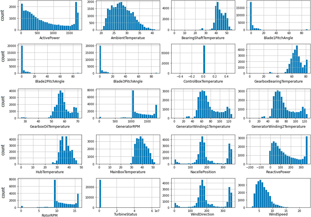
FIGURE 4. Histograms charts of the features included in the wind power dataset.

FIGURE 5

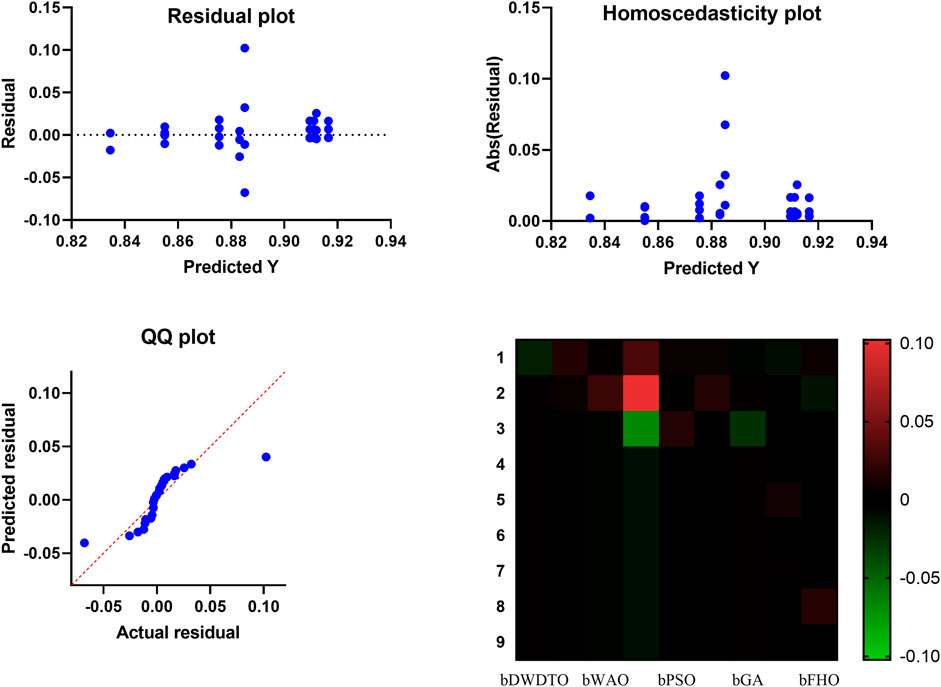
FIGURE 5. Visualizing the proposed feature selection method results.

Algorithm 2. The proposed binary bDWDTO algorithm.

1: Initialize the parameters of GADTO algorithm

2: Convert the resulting best solution to binary [0,1]

3: Evaluate the fitness of the resulting solutions

4: Train KNN to assess the resulting solutions

5: Sett = 1

6: while t ≤ Max_iteration do

7: Run GADTO algorithm to get best solutions X_best

8: Convert best solutions to binary using the following equation:

$\begin{array}{ll}\hfill & S_{\mathit{binary}}=\left\{\begin{array}{cc}1\hfill & \text{if\hspace{0.17em}}F\left(X_{\mathit{best}}\right)\ge 0.5\hfill \\ 0\hfill & otherwise\hfill \end{array}\right.,\hfill \\ \hfill & F\left(X_{\mathit{Best}}\right)=\frac{1}{1+e^{-10\left(X_{\mathit{Best}}-0.5\right)}}\hfill \end{array}$

9: Calculate the fitness value

10: Update the parameters of GADTO algorithm

11: Update t = t + 1

12: end while

13: Return best set of features

There are 118,224 sample points gathered in the dataset with 20 features each. To determine the relationship between the alternate input variables, the following equation is used to determine the Pearson coefficients.

$\rho \left(A,B\right)=\frac{E\left[\left(A-\mu A\right)\left(B-\mu B\right)\right]}{\sqrt{{\sum }_{i=1}^n{\left(A_i-\mu A\right)}^2}\sqrt{{\sum }_{i=1}^n{\left(B_i-\mu B\right)}^2}}(18)$

To predict the wind turbines’ output power by utilizing many correlated variables as input quantities, this research proposes an ensemble model based on LSTM, GRU, and BiLSTM to maintain a selected set of features for effective prediction. The proposed ensemble model deals with both time-dependent and historically-dependent data.

4.2 Configuration parameters of optimization algorithms

The conducted experiments utilize a set of optimization algorithms for comparison purposes. These algorithms are the standard DTO (Takieldeen et al., 2022), the standard WOA (Mirjalili and Lewis, 2016), grey wolf optimization (GWO) (Mirjalili et al., 2014), firefly algorithm (FA) (Ariyaratne and Fernando, 2023), particle swarm optimization (PSO) (Awange et al., 2018), the genetic algorithm (Immanuel and Chakraborty, 2019), the JAYA algorithm (Venkata Rao and Venkata Rao, 2019), and the Fire Hawk Optimizer (FHO) algorithm (Azizi et al., 2023). The basic configuration parameters of these algorithms are presented in Table 1.

TABLE 1

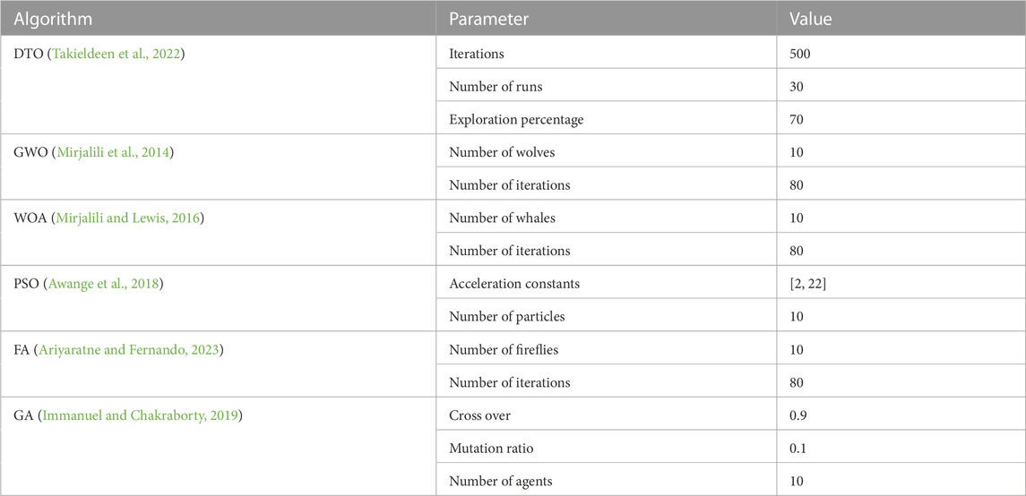
TABLE 1. The settings of the parameters of the optimization algorithms.

4.3 Evaluation metrics

The evaluation metrics of the results achieved by the conducted experiments are categorized into two sets of metrics. The first set of metrics is presented in Table 2 and used to assess the feature selection results. This set of metrics includes best fitness, worst fitness, average error, average fitness size, standard deviation, and average fitness. The second set of metrics is presented in Table 3, which includes mean bias error (MBE), root means square error (RMSE), mean absolute percentage error (MAPE), mean absolute error (MAE), R-squared (R²), determine agreement (WI), Nash Sutcliffe Efficiency (NSE), relative RMSE (RRMSE), and Pearson’s correlation coefficient (r).

TABLE 2

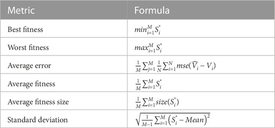
TABLE 2. Formulas of the metrics used in evaluating the feature selection results.

TABLE 3

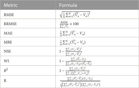
TABLE 3. Formulas of the metrics used in evaluating the wind power prediction results.

4.4 Evaluating the feature selection results

The utility of the developed wind power prediction model will be tested, and its benefits will be quantified in this research. It is important to evaluate how well the proposed DWDTO algorithm works. Experiments were performed using the configuration parameters presented in the previous section. Table 4 presents the evaluation of the proposed feature selection method compared to current feature selection methods in the literature. Considering fitness, select size, and error, the outcomes show that the proposed feature selection strategy is effective. With a “Best fitness” of 0.822, the algorithm appears to have located a solution that excels at the specified goal. With an “Average select size” of 0.810, it is clear that the approach has chosen an appropriate number of features for excellent accuracy without resorting to overfitting. The “Average error” of 0.837 indicates that the number of errors caused by the model has decreased according to the chosen features. Yet, given that the mistake rate is not zero, there is space for enhancement. The average fitness score of 0.920 for the attributes that were chosen is relatively high. An “Std fitness” of 0.742 shows a wide range of values for the specified features’ fitness metrics. This indicates that the fitness score may vary greatly depending on the characteristic. Finally, the “Worst Fitness” value of 0.920 is encouraging because it indicates that the feature selection technique has not chosen any features with a meager fitness score. The proposed feature selection method has selected a subset of characteristics with a high fitness score and low error rate. However, the substantial diversity in fitness scores and the non-zero error rate implies that more progress is possible. It is possible that the method’s performance could benefit from more research and refinement.

TABLE 4

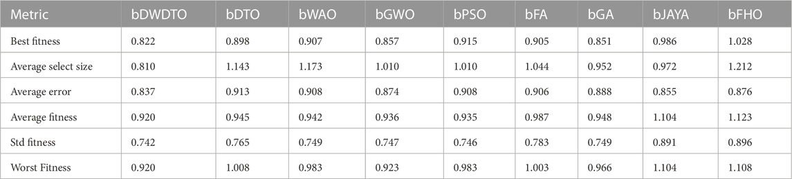
TABLE 4. The results of the proposed feature selection method.

In addition, other statistical tests, such as the one-way analysis of variance (ANOVA) and Wilcoxon signed-rank tests, are performed to study the difference between the proposed methodology and the other methods. These tests’ results are presented in Table 5; Table 6, respectively. In these tables, the indicator of difference is the p-value which is lower than 0.005, which proves the statistical difference. Applying the ANOVA test to the outcomes of the proposed feature selection approach yielded the following findings. The number of groups in the treatment is represented by the “DF” (degrees of freedom) value of 8, and the “SS” (sum of squares) value of 0.05862 indicates the total variation explained by the therapy. F (DFn, DFd) is the F statistic value obtained by dividing the “MS” (mean square) for the treatment by the “MS” (mean square) for the residual, which equals 0.007328. The F-value, in this case, is 25.38, and the p-value is less than 0.0001. Therefore, there are statistically significant differences between the treatment groups. The “SS” value of 0.02078 for the residual represents the remaining unexplained data variation after controlling for the treatment effect. The residuals have 72 “DF,” or degrees of freedom, and each degree of freedom has an unexplained variance of 0.0002887 “MS.” Lastly, the sum of the squares of the standard deviations (SS) is 0.07941, which is the overall variation in the data. The total degree of freedom (or “DF”) across the entire dataset is 80. These findings show that the proposed feature selection strategy has achieved statistically significant variations in treatment outcomes. The therapy significantly affects the outcome of the feature selection approach, as seen by the high F-value and low p-value. Furthermore, the residual values show the remaining unexplained variation in the data, suggesting that this area may benefit from additional study.

TABLE 5

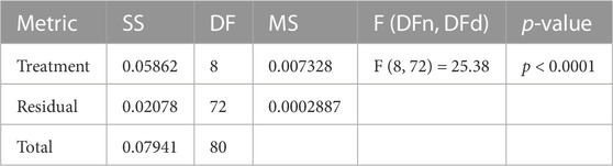
TABLE 5. Analysis results using ANOVA test.

TABLE 6

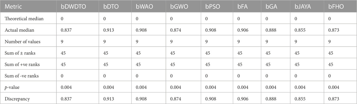
TABLE 6. Analysis results using Wilcoxon test.

Using the Wilcoxon signed-rank test, we compared the outcomes of the proposed feature selection approach to those of a baseline set of methods. The median predicted value of the dissimilarities between the matched samples, denoted by “Theoretical median,” is zero. The median observed discrepancy between the paired samples (the “Real median”) is 0.837. The “Number of values” indicates that nine pairs of data were used for the analysis. The sum of signed ranks is the sum of the absolute values of the rankings of the differences between the matched samples. We can add up the positive and negative differences rankings and call those the “Sum of +ve ranks” and the “Sum of -ve ranks,” respectively. It appears that there were largely positive differences between the matched samples because the “Sum of signed rankings” is 45 and the “Sum of -ve ranks” is 0, respectively. For a null hypothesis to be correct, the likelihood of generating a test statistic as extreme as the observed statistic is 0.004. The lack of statistical significance between the paired samples is the null hypothesis in this example. Statistically, there is a substantial difference between the paired samples, as indicated by the low p-value, which allows the null hypothesis to be rejected at the 0.05 level of significance. When comparing the observed median to the theoretical median, the discrepancy (or “Discrepancy”) equals 0.837. This number indicates the variation between the two samples in a set. A low p-value indicates that there is likely to be a statistically significant difference between the two samples. When there is a positive difference between paired samples, as shown by the “Sum of signed rankings” and “Sum of +ve ranks,” it is possible that the proposed feature selection approach worked better on the selected features than the non-selected ones. The two groups have an apparent disparity, as seen by the 0.837 median difference.

On the other hand, Figure 5 shows the accuracy of the wind power prediction. In this figure, many graphical tools can be used to examine the results of an ANOVA and analyze the model’s assumptions while assessing a feature selection approach. A heatmap plot is a kind of data visualization that uses color to convey information about the importance of certain features. Data patterns can be discovered, and the feature selection method’s efficacy evaluated using the heatmap. Features that are highly correlated and relevant to the outcome will be clustered together clearly in a heatmap, as with a high-performance feature selection approach. However, when testing the normality assumption of an ANOVA model, a QQ plot can be helpful. The residuals’ distribution is compared to a normal distribution, and outliers are flagged if they are found. The normality assumption holds if the residuals on the QQ plot form a straight line. If the line is not straight, the residuals may not be normally distributed, calling into question the reliability of the ANOVA findings. The assumption of homoscedasticity in the ANOVA model states that the residual variance should be the same for all predictor variable values. A residual plot can be used to test for homoscedasticity. The residual plot contrasts the actual values with the expected ones, and a homoscedastic plot illustrates a uniform distribution of data points around the zero line. Heteroscedasticity, which might compromise the reliability of ANOVA results, is indicated by a plot with a fan shape or an increasing or decreasing spread of points. Heatmap plots, QQ plots, and residual plots are just a few examples of graphical tools that can be used to evaluate the efficacy of feature selection strategies and the validity of the ANOVA model’s assumptions. A thorough examination of these plots allows researchers to spot problems in the data or the model and make corrections that will increase confidence in the ANOVA findings.

In addition, Figure 6 shows the average error in feature selection using the proposed method and the other competitor methods. As seen in this figure, the proposed feature selection algorithm gets the lowest average error, suggesting it does better than the different algorithms in picking relevant characteristics for the prediction task. The scatter figure demonstrates that the proposed feature selection algorithm obtains the lowest average error across multiple datasets, proving its effectiveness and generalizability. That the algorithm can identify the most informative features for the prediction task and reduce data dimensionality without compromising accuracy is a significant indication of the algorithm’s trustworthiness. Also, the graphic clearly shows how the proposed feature selection algorithm compares to the other algorithms utilized in the study and where the discrepancies lie. This knowledge can be used to determine the best feature selection strategy for a given prediction problem, considering the dataset and prediction method in question. The proposed approach achieves the lowest average error and surpasses the other algorithms in selecting relevant features for the prediction job, as shown by a plot of the average error of the algorithms employed in feature selection compared to the proposed algorithm. This demonstrates that the proposed approach is an efficient and trustworthy tool for feature selection, which can be utilized to enhance the precision and productivity of prediction algorithms across a wide range of applications.

FIGURE 6

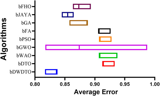
FIGURE 6. The average error of the feature selection results based on the proposed and other feature selection methods.

4.5 Prediction results

The prediction results listed in Table 7 based on the adopted evaluation metrics show the superiority and effectiveness of the proposed optimized ensemble model compared to other models. Compared to the LSTM, BiLSTM, and GRU prediction models, the results of the suggested ensemble model for wind power prediction demonstrate outstanding accuracy and performance. With an RMSE of 0.0022, the suggested model has a relatively modest average deviation from the true values in its predictions. With an R2 of 0.9999, the model provides a close fit to the data, leaving little room for error. The model’s correctness is further supported by the MBE of 7.6E-06 and the MAE of 0.0003. The high WI value of 0.9991 and R-value of 0.9999 shows that the values predicted and observed are highly correlated. An NSE of 0.9999 means the suggested model captures the observed data’s variability remarkably well. The RRMSE of 0.4185 further shows that the proposed ensemble model has a small relative error compared to the average of the real values. Our findings show that the proposed ensemble model excels in all respects over the state-of-the-art LSTM, BiLSTM, and GRU prediction models. There is a good chance that this model could be used in real-world wind power forecast applications due to its high accuracy and significant connection with actual data. These findings have the potential to aid in the selection of prediction models for wind power generation and shed light on the creation of more precise and efficient models for forecasting renewable energy.

TABLE 7

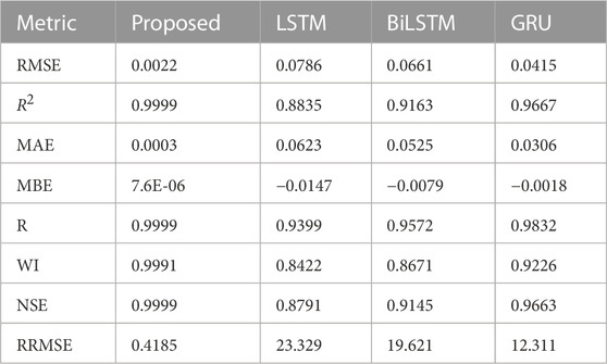
TABLE 7. The prediction results using the proposed optimized ensemble.

Similar to the evaluation of the feature selection results, the results of the wind power prediction are statistically evaluated in terms of the ANOVA, Wilcoxon, and statistical analysis as presented in Table 8, Table 9, and Table 10, respectively. The results in these tables confirm the statistical significance and difference of the proposed methodology compared to the other recent methods.

TABLE 8

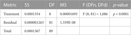
TABLE 8. Analysis of the achieved prediction results using ANOVA test.

TABLE 9

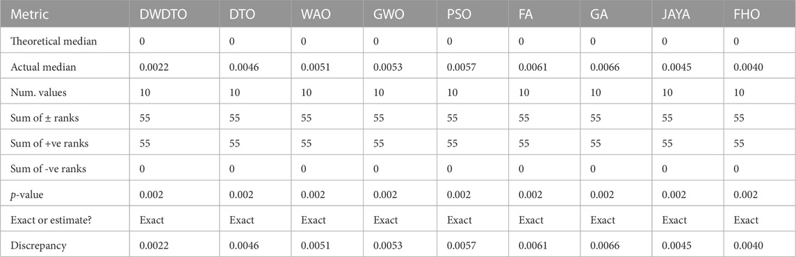
TABLE 9. Analysis of the achieved prediction results using Wilcoxon test.

TABLE 10

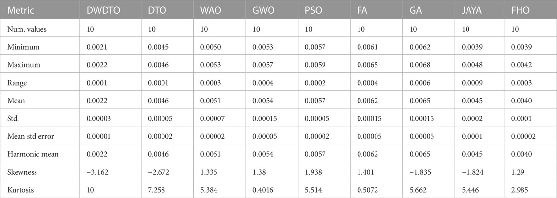
TABLE 10. Statistical analysis of the achieved prediction results.

On the other hand, a set of figures was generated to show this finding to emphasize the accuracy of the prediction results achieved by the proposed approach. Figure 7; Figure 8; Figure 9; Figure 10 show the prediction errors using the proposed approach with comparison to other approaches. It can be easily noted in these figures that the proposed methodology is superior in predicting wind power.

FIGURE 7

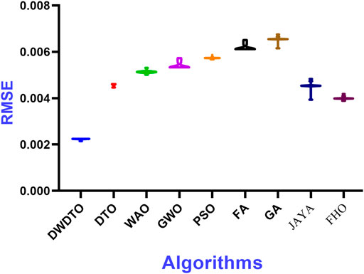
FIGURE 7. RMSE values calculated for the results achieved by the proposed optimization algorithm.

FIGURE 8

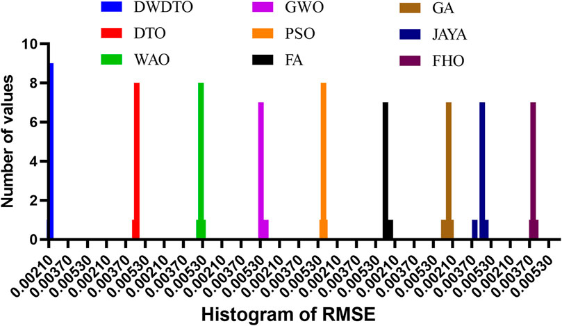
FIGURE 8. RMSE histogram values calculated for the results achieved by the proposed optimization algorithm.

FIGURE 9

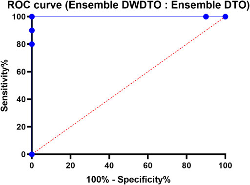
FIGURE 9. The receiver operating characteristic curve of the proposed ensemble model versus another ensemble model.

FIGURE 10

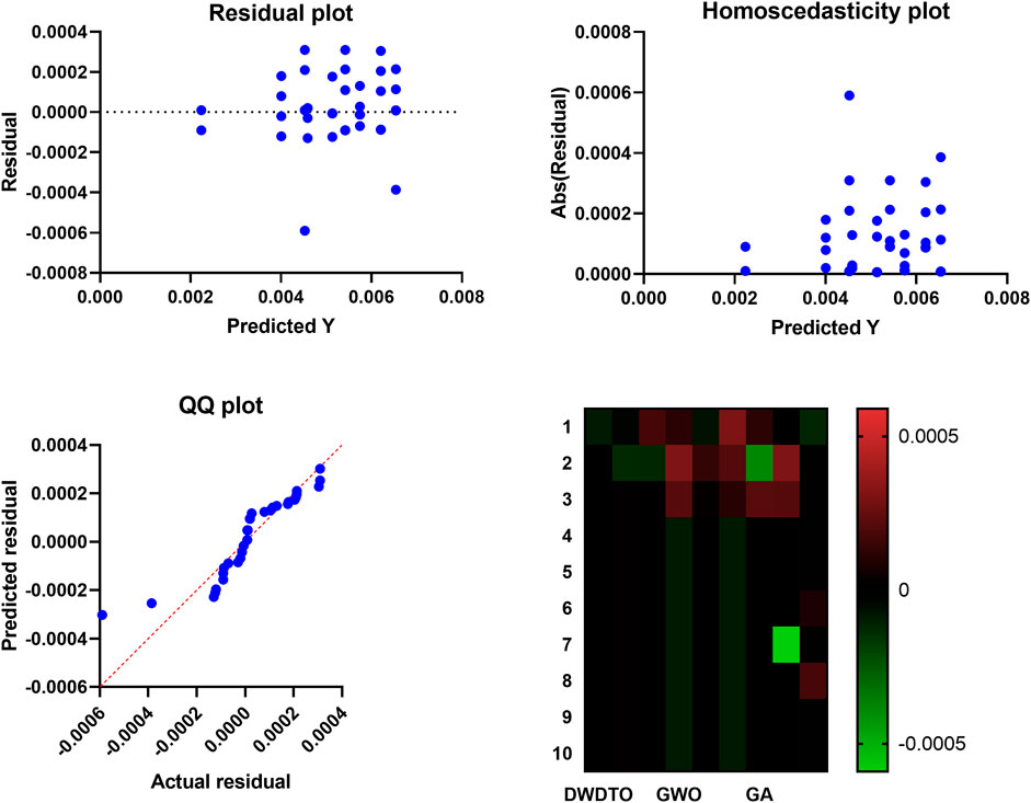
FIGURE 10. Visualizing the proposed optimized ensemble method prediction results.

The plots of RMSE values show that the proposed method achieves the least range of RMSE values compared to the other methods. This means the proposed method outperforms the competing methods on all datasets examined. The charts also make it easy to see the differences between the methods by displaying the range of RMSE values attained by each. The histogram of RMSE values further supports the proposed method’s improved performance. The suggested method consistently achieves excellent accuracy throughout the investigated datasets, as shown by the histogram, which shows that most RMSE values generated by the method are concentrated around a small range of values. The RMSE values for the other approaches are more dispersed, with some datasets obtaining very high error rates. This indicates that the proposed method is superior to the alternatives in terms of robustness, reliability, and flexibility regarding datasets. Plots of the RMSE values and a histogram show the suggested methodology’s superior performance over the other methods. The histogram shows that the suggested method provides high accuracy consistently across different datasets, with a restricted range of RMSE values and a concentration of values around that range. Insights into constructing more accurate and efficient regression models can be gained from these findings, making them crucial for influencing the selection of approaches for regression tasks.

Here, we contrast the performance of an ensemble model optimized with the DTO method with that of the proposed ensemble model optimized with the DWDTO algorithm. The Receiver Operating Characteristic (ROC) curve is utilized to visualize how well the proposed model is performing. This curve displays the sensitivity versus the false positive rate (1—specificity) for various cutoffs in the prediction process. Examining the ROC curve reveals that the proposed ensemble model employing the DWDTO method outperforms the one employing the DTO technique. The receiver operating characteristic (ROC) curve for the proposed ensemble model using the DWDTO method demonstrates that the model achieves a greater true positive rate (sensitivity) than the ensemble model using the DTO algorithm at lower false positive rates (1—specificity). It follows that the proposed ensemble model outperforms the ensemble model trained using the DTO approach in its capacity to correctly detect positive events (high wind power generation) while avoiding false positive cases (low wind power generation). Higher specificity and sensitivity values on the ROC curve demonstrate that the proposed ensemble model optimized with the DWDTO algorithm performs better than that optimized with the DTO strategy. This shows that the proposed model is more trustworthy for decision-making in energy systems since it can predict wind power generation more accurately and with less likelihood of false positives or negatives.

5 Conclusion

This research proposes an optimized ensemble model based on a novel optimization algorithm. The proposed optimization methodology is referred to as DWDTO. This algorithm is used in feature selection and optimization of the ensemble weights to improve the precision of wind power forecasting. A dataset publicly available on Kaggle is utilized to prove the proposed methodology’s effectiveness. The proposed optimized ensemble is the foundational forecasting model for the non-linear connection between data-variable features and wind power. The proposed DWDTO is developed for determining the ensemble weights’ optimal values. It is shown that the proposed optimized ensemble model is the most effective of other developed comparative forecasting models in terms of improving prediction error. The RMSE of the proposed model was the lowest of the forecasting models in all the conducted experiments, with a value of 0.0022. Wind power studies using data from a single wind farm reveal that the proposed prediction model is effective and that the mapping connection of the created power prediction model is straightforward. The future perspective is to evaluate the proposed methodology using a larger dataset to show its generalization.

Data availability statement

The dataset of wind power forecasting used in this study can be found on Kaggle: https://www.kaggle.608com/datasets/theforcecoder/wind-power-forecasting.

Author contributions

Methodology, AbA, E-SE-K and AI; Software, E-SE-K; Data curation, AF and AI; Writing—original draft, AbA, E-SE-K; Writing—review & editing, AmA and DK; Funding acquisition, AmA and DK. All authors have read and agreed to the published version of the manuscript.

Funding

Princess Nourah Bint Abdulrahman University Researchers Supporting Project number (PNURSP 2023R 308), Princess Nourah Bint Abdulrahman University, Riyadh, Saudi Arabia.

Conflict of interest

The authors declare that the research was conducted in the absence of any commercial or financial relationships that could be construed as a potential conflict of interest.

Publisher’s note

All claims expressed in this article are solely those of the authors and do not necessarily represent those of their affiliated organizations, or those of the publisher, the editors and the reviewers. Any product that may be evaluated in this article, or claim that may be made by its manufacturer, is not guaranteed or endorsed by the publisher.

References

Abdelbaky, M. A., Liu, X., and Jiang, D. (2020). Design and implementation of partial offline fuzzy model-predictive pitch controller for large-scale wind-turbines. Renew. Energy145, 981–996. doi:10.1016/j.renene.2019.05.074

CrossRef Full Text | Google Scholar

Akhter, M. N., Mekhilef, S., Mokhlis, H., Ali, R., Usama, M., Muhammad, M. A., et al. (2022). A hybrid deep learning method for an hour ahead power output forecasting of three different photovoltaic systems. Appl. Energy307, 118185. doi:10.1016/j.apenergy.2021.118185

CrossRef Full Text | Google Scholar

Alhussan, A. A., Khafaga, D. S., El-Kenawy, E.-S. M., Ibrahim, A., Eid, M. M., and Abdelhamid, A. A. (2022). Pothole and plain road classification using adaptive mutation dipper throated optimization and transfer learning for self driving cars. IEEE Access10, 84188–84211. doi:10.1109/ACCESS.2022.3196660

CrossRef Full Text | Google Scholar

An, G., Jiang, Z., Chen, L., Cao, X., Li, Z., Zhao, Y., et al. (2021). Ultra short-term wind power forecasting based on sparrow search algorithm optimization deep extreme learning machine. Sustainability13, 10453. doi:10.3390/su131810453

CrossRef Full Text | Google Scholar

Ariyaratne, M., and Fernando, T. (2023). A comprehensive review of the firefly algorithms for data clustering. Cham: Springer International Publishing, 217. doi:10.1007/978-3-031-09835-2_12

CrossRef Full Text | Google Scholar

Awange, J. L., Paláncz, B., Lewis, R. H., and Völgyesi, L. (2018). “enParticle swarm optimization,” in Mathematical geosciences: Hybrid symbolic-numeric methods. Editors J. L. Awange, B. Paláncz, R. H. Lewis, and L. Völgyesi (Cham: Springer International Publishing), 167–184. doi:10.1007/978-3-319-67371-4/TNQDotTNQ/6

CrossRef Full Text | Google Scholar

Azizi, M., Talatahari, S., and Gandomi, A. H. (2023). Fire Hawk optimizer: A novel metaheuristic algorithm. Artif. Intell. Rev.56, 287–363. doi:10.1007/s10462-022-10173-w

CrossRef Full Text | Google Scholar

Bhaskarpandit, S. (2020). Wind power forecasting. Available at https://www.kaggle.com/datasets/theforcecoder/wind-power-forecasting.

Google Scholar

Chen, G., Tang, B., Zeng, X., Zhou, P., Kang, P., and Long, H. (2022). Short-term wind speed forecasting based on long short-term memory and improved BP neural network. Int. J. Electr. Power and Energy Syst.134, 107365. doi:10.1016/j.ijepes.2021.107365

CrossRef Full Text | Google Scholar

Demolli, H., Dokuz, A. S., Ecemis, A., and Gokcek, M. (2019). Wind power forecasting based on daily wind speed data using machine learning algorithms. Energy Convers. Manag.198, 111823. doi:10.1016/j.enconman.2019.111823

CrossRef Full Text | Google Scholar

Duan, J., Wang, P., Ma, W., Tian, X., Fang, S., Cheng, Y., et al. (2021a). Short-term wind power forecasting using the hybrid model of improved variational mode decomposition and Correntropy Long Short -term memory neural network. Energy214, 118980. doi:10.1016/j.energy.2020.118980

CrossRef Full Text | Google Scholar

Duan, J., Zuo, H., Bai, Y., Duan, J., Chang, M., and Chen, B. (2021b). Short-term wind speed forecasting using recurrent neural networks with error correction. Energy217, 119397. doi:10.1016/j.energy.2020.119397

CrossRef Full Text | Google Scholar

El-kenawy, E.-S. M., Albalawi, F., Ward, S. A., Ghoneim, S. S. M., Eid, M. M., Abdelhamid, A. A., et al. (2022). Feature selection and classification of transformer faults based on novel meta-heuristic algorithm. Mathematics10, 3144. doi:10.3390/math10173144

CrossRef Full Text | Google Scholar

El-Kenawy, E.-S. M., Mirjalili, S., Abdelhamid, A. A., Ibrahim, A., Khodadadi, N., and Eid, M. M. (2022a). Meta-heuristic optimization and keystroke dynamics for authentication of smartphone users. Mathematics10, 2912. doi:10.3390/math10162912

CrossRef Full Text | Google Scholar

El-Kenawy, E.-S. M., Mirjalili, S., Alassery, F., Zhang, Y.-D., Eid, M. M., El-Mashad, S. Y., et al. (2022b). Novel meta-heuristic algorithm for feature selection, unconstrained functions and engineering problems. IEEE Access10, 40536–40555. doi:10.1109/access.2022.3166901

CrossRef Full Text | Google Scholar

Ewees, A. A., Al-qaness, M. A., Abualigah, L., and Elaziz, M. A. (2022). HBO-LSTM: Optimized long short term memory with heap-based optimizer for wind power forecasting. Energy Convers. Manag.268, 116022. doi:10.1016/j.enconman.2022.116022

CrossRef Full Text | Google Scholar

Han, L., Jing, H., Zhang, R., and Gao, Z. (2019). Wind power forecast based on improved Long Short Term Memory network. Energy189, 116300. doi:10.1016/j.energy.2019.116300

CrossRef Full Text | Google Scholar

Huang, F., Li, Z., Xiang, S., and Wang, R. (2021). A new wind power forecasting algorithm based on long short-term memory neural network. Int. Trans. Electr. Energy Syst.31, 1. doi:10.1002/2050-7038.13233

CrossRef Full Text | Google Scholar

Immanuel, S. D., and Chakraborty, U. K. (2019). “Genetic algorithm: An approach on optimization,” in International Conference on Communication and Electronics Systems (ICCES). 22-24 June 2022, Germany, ICCES, 701. doi:10.1109/ICCES45898.2019.9002372

CrossRef Full Text | Google Scholar

Khafaga, D. S., Alhussan, A. A., El-Kenawy, E.-S. M., Ibrahim, A., Eid, M. M., and Abdelhamid, A. A. (2022). Solving optimization problems of metamaterial and double t-shape antennas using advanced meta-heuristics algorithms. IEEE Access10, 74449–74471. doi:10.1109/ACCESS.2022.3190508

CrossRef Full Text | Google Scholar

Khan, M., Al-Ammar, E. A., Naeem, M. R., Ko, W., Choi, H.-J., and Kang, H.-K. (2021). Forecasting renewable energy for environmental resilience through computational intelligence. PLOS ONE16, e0256381. doi:10.1371/journal.pone.0256381

PubMed Abstract | CrossRef Full Text | Google Scholar

Kisvari, A., Lin, Z., and Liu, X. (2021). Wind power forecasting – a data-driven method along with gated recurrent neural network. Renew. Energy163, 1895–1909. doi:10.1016/j.renene.2020.10.119

CrossRef Full Text | Google Scholar

Kong, X., Ma, L., Liu, X., Abdelbaky, M. A., and Wu, Q. (2020). Wind turbine control using nonlinear economic model predictive control over all operating regions. Energies13, 184. doi:10.3390/en13010184

CrossRef Full Text | Google Scholar

Kong, X., Ma, L., Wang, C., Guo, S., Abdelbaky, M. A., Liu, X., et al. (2022). Large-scale wind farm control using distributed economic model predictive scheme. Renew. Energy181, 581–591. doi:10.1016/j.renene.2021.09.048

CrossRef Full Text | Google Scholar

Kumar Ganti, P., Naik, H., and Kanungo Barada, M. (2022). Environmental impact analysis and enhancement of factors affecting the photovoltaic (PV) energy utilization in mining industry by sparrow search optimization based gradient boosting decision tree approachEnergy244, 122561. doi:10.1016/j.energy.2021.122561

CrossRef Full Text | Google Scholar

Kusiak, A., Zhang, Z., and Verma, A. (2013). Prediction, operations, and condition monitoring in wind energy. Energy60, 1–12. doi:10.1016/j.energy.2013.07.051

CrossRef Full Text | Google Scholar

Li, F., Zheng, H., and Li, X. (2022). A novel hybrid model for multi-step ahead photovoltaic power prediction based on conditional time series generative adversarial networks. Renew. Energy199, 560–586. doi:10.1016/j.renene.2022.08.134

CrossRef Full Text | Google Scholar

Li, L.-L., Zhao, X., Tseng, M.-L., and Tan, R. R. (2020). Short-term wind power forecasting based on support vector machine with improved dragonfly algorithm. J. Clean. Prod.242, 118447. doi:10.1016/j.jclepro.2019.118447

CrossRef Full Text | Google Scholar

Liu, G., Shu, C., Liang, Z., Peng, B., and Cheng, L. (2021a). A modified sparrow search algorithm with application in 3d route planning for UAV. Sensors21, 1224. doi:10.3390/s21041224

PubMed Abstract | CrossRef Full Text | Google Scholar

Liu, M.-D., Ding, L., and Bai, Y.-L. (2021b). Application of hybrid model based on empirical mode decomposition, novel recurrent neural networks and the ARIMA to wind speed prediction. Energy Convers. Manag.233, 113917. doi:10.1016/j.enconman.2021.113917

CrossRef Full Text | Google Scholar

Liu, X., Zhang, H., Kong, X., and Lee, K. Y. (2020). Wind speed forecasting using deep neural network with feature selection. Neurocomputing397, 393–403. doi:10.1016/j.neucom.2019.08.108

CrossRef Full Text | Google Scholar

Majidi Nezhad, M., Heydari, A., Groppi, D., Cumo, F., and Astiaso Garcia, D. (2020). Wind source potential assessment using sentinel 1 satellite and a new forecasting model based on machine learning: A case study sardinia islands. Renew. Energy155, 212–224. doi:10.1016/j.renene.2020.03.148

CrossRef Full Text | Google Scholar

Memarzadeh, G., and Keynia, F. (2020). A new short-term wind speed forecasting method based on fine-tuned LSTM neural network and optimal input sets. Energy Convers. Manag.213, 112824. doi:10.1016/j.enconman.2020.112824

CrossRef Full Text | Google Scholar

Mirjalili, S., and Lewis, A. (2016). The whale optimization algorithm. Adv. Eng. Softw.95, 51–67. doi:10.1016/j.advengsoft.2016.01.008

CrossRef Full Text | Google Scholar

Mirjalili, S., Mirjalili, S. M., and Lewis, A. (2014). Grey wolf optimizer. Adv. Eng. Softw.69, 46–61. doi:10.1016/j.advengsoft.2013.12.007

CrossRef Full Text | Google Scholar

Neshat, M., Nezhad, M. M., Abbasnejad, E., Mirjalili, S., Tjernberg, L. B., Astiaso Garcia, D., et al. (2021). A deep learning-based evolutionary model for short-term wind speed forecasting: A case study of the lillgrund offshore wind farm. Energy Convers. Manag.236, 114002. doi:10.1016/j.enconman.2021.114002

CrossRef Full Text | Google Scholar

Peng, X., Wang, H., Lang, J., Li, W., Xu, Q., Zhang, Z., et al. (2021). EALSTM-QR: Interval wind-power prediction model based on numerical weather prediction and deep learning. Energy220, 119692. doi:10.1016/j.energy.2020.119692

CrossRef Full Text | Google Scholar

Qing, X., and Niu, Y. (2018). Hourly day-ahead solar irradiance prediction using weather forecasts by LSTM. Energy148, 461–468. doi:10.1016/j.energy.2018.01.177

CrossRef Full Text | Google Scholar

Shahid, F., Zameer, A., and Muneeb, M. (2021). A novel genetic LSTM model for wind power forecast. Energy223, 120069. doi:10.1016/j.energy.2021.120069

CrossRef Full Text | Google Scholar

Takieldeen, E., El-kenawy, A., M., Hadwan, M., and Zaki, M. R. (2022). Dipper throated optimization algorithm for unconstrained function and feature selection. Comput. Mater. Continua72, 1465–1481. doi:10.32604/cmc.2022.026026

CrossRef Full Text | Google Scholar

Tian, Z., and Chen, H. (2021). A novel decomposition-ensemble prediction model for ultra-short-term wind speed. Energy Convers. Manag.248, 114775. doi:10.1016/j.enconman.2021.114775

CrossRef Full Text | Google Scholar

Tian, Z. (2020). Short-term wind speed prediction based on LMD and improved FA optimized combined kernel function LSSVM. Eng. Appl. Artif. Intell.91, 103573. doi:10.1016/j.engappai.2020.103573

CrossRef Full Text | Google Scholar

Tian, Z., and Wang, J. (2022). Variable frequency wind speed trend prediction system based on combined neural network and improved multi-objective optimization algorithm. Energy254, 124249. doi:10.1016/j.energy.2022.124249

CrossRef Full Text | Google Scholar

Venkata Rao, R. (2019). “enJaya optimization algorithm and its variants,” in Jaya: An advanced optimization algorithm and its engineering applications. Editor R. Venkata Rao (Cham: Springer International Publishing), 9–58. doi:10.1007/978-3-319-78922-4_2

CrossRef Full Text | Google Scholar

Wang, Y., Zou, R., Liu, F., Zhang, L., and Liu, Q. (2021). A review of wind speed and wind power forecasting with deep neural networks. Appl. Energy304, 117766. doi:10.1016/j.apenergy.2021.117766

CrossRef Full Text | Google Scholar

Xiang, L., Liu, J., Yang, X., Hu, A., and Su, H. (2022). Ultra-short term wind power prediction applying a novel model named SATCN-LSTM. Energy Convers. Manag.252, 115036. doi:10.1016/j.enconman.2021.115036

CrossRef Full Text | Google Scholar

Xu, W., Liu, P., Cheng, L., Zhou, Y., Xia, Q., Gong, Y., et al. (2021). Multi-step wind speed prediction by combining a WRF simulation and an error correction strategy. Renew. Energy163, 772–782. doi:10.1016/j.renene.2020.09.032

CrossRef Full Text | Google Scholar

Xue, J., and Shen, B. (2020). A novel swarm intelligence optimization approach: Sparrow search algorithm. Syst. Sci. Control Eng.8, 22–34. doi:10.1080/21642583.2019.1708830

CrossRef Full Text | Google Scholar

Yang, Q., Liu, P., Zhang, J., and Dong, N. (2022). Combined heat and power economic dispatch using an adaptive cuckoo search with differential evolution mutation. Appl. Energy307, 118057. doi:10.1016/j.apenergy.2021.118057

CrossRef Full Text | Google Scholar

Zhang, C., and Ding, S. (2021). A stochastic configuration network based on chaotic sparrow search algorithm. Knowledge-Based Syst.220, 106924. doi:10.1016/j.knosys.2021.106924

CrossRef Full Text | Google Scholar

Zhang, J., Liu, D., Li, Z., Han, X., Liu, H., Dong, C., et al. (2021). Power prediction of a wind farm cluster based on spatiotemporal correlations. Appl. Energy302, 117568. doi:10.1016/j.apenergy.2021.117568

CrossRef Full Text | Google Scholar

Zhang, J., Yan, J., Infield, D., Liu, Y., and Lien, F.-s. (2019). Short-term forecasting and uncertainty analysis of wind turbine power based on long short-term memory network and Gaussian mixture model. Appl. Energy241, 229–244. doi:10.1016/j.apenergy.2019.03.044

CrossRef Full Text | Google Scholar

Zhang, Y., Pan, G., Chen, B., Han, J., Zhao, Y., and Zhang, C. (2020). Short-term wind speed prediction model based on GA-ANN improved by VMD. Renew. Energy156, 1373–1388. doi:10.1016/j.renene.2019.12.047

CrossRef Full Text | Google Scholar