Flexible and optimized operation of integrated energy systems based on exergy analysis and pipeline dynamic characteristics

1 Introduction

To solve the increasingly serious environmental problems, achieving “carbon peak and carbon neutrality” sooner has become the consensus of all countries worldwide (Chen et al., 2021; Alabi et al., 2022; Woon et al., 2023). As the energy sector is a major source of carbon emissions, promoting energy transformation and building clean, efficient, and sustainable energy systems has become an urgent priority (Berjawi et al., 2021; Liu et al., 2021). The integrated energy system (IES) not only meets the energy supply of diversified loads but also reduces losses and improves energy efficiency through multi-energy complementarity to achieve the purpose of energy conservation and emission reduction (Wang et al., 2019; Zhu et al., 2021; Bie et al., 2022). Therefore, constructing an efficient and a high-quality IES is an important measure to solve the current problems of environmental pollution and resource shortage.

There has been a lot of research on the modeling, planning, and economic operation of the IES. First, the perturbation chain statistical associating fluid theory (PC-SAFT) was used to predict the thermodynamic properties of natural gas mixtures. Then, a multilayer perceptron neural network model was established to predict the natural gas demand at any ambient temperature. A new simulation method for a non-stationary natural gas distribution network was proposed to predict the response of distribution pipelines to environmental temperature changes (Gord et al., 2013; Farzaneh-Gord and Rahbari. 2018). In the study by Chen et al. (2020), a new scheduling model of the electric–thermal–gas coupling system based on the unified energy path theory was proposed. This model can explore the dynamic characteristics of heating and natural gas networks to improve the flexibility of the system. In the study by Xu et al. (2020), taking the energy hub as the distributed decision-maker, a distributed multi-time and multi-energy operation model was proposed to achieve the electric–gas–thermal IES optimal coordination under the coupling of a multi-energy infrastructure. In the study by Liu et al. (2018), the optimal scheduling problem of a regional IES, which included energy conversion and storage equipment, was analyzed using an energy storage equipment to decouple thermoelectric connections and modeling the randomness of the renewable power output by the scenario analysis method. In the study by Fan et al. (2023), the robust optimization theory (Qiu et al., 2022; Zhao et al., 2022) was introduced to deal with the fluctuation problem of wind power output, and a multi-type energy storage IES bi-level (B-L) optimization model was established to effectively integrate distributed energy resources. The above research is based on the first law of thermodynamics and takes energy as the starting point to conduct an in-depth mechanism analysis within various subsystems in the IES.

Exergy is theoretically the part of energy that is converted into useful energy, which reflects the degree of available energy. This also means that exergy can reflect the magnitude of the “quantity” and the level of “quality” in energy. Therefore, based on the second law of thermodynamics, the work potential of an equipment can be more accurately characterized by exergy analysis, and the energy utilization rate of the system can be reflected. Li et al. (2022) combined network characteristics with exergy and proposed an equivalent transformation method of the exergy flow model of the regional heat network, which has a single-layer structure like the electric and gas distribution networks, and the unified analysis of the exergy flow of the regional integrated energy system (RIES) can be realized. The unified calculation model of exergy flow realizes the efficient solution of exergy flow distribution. In the study by Chen et al. (2020), based on energy axiomatization, the steady-state transport process of exergy in the gas–thermal network has been described as an equivalent circuit. In the study by Li et al. (2022), based on the idea of “flow,” the connection between supply, network, and demand was established, and a modeling method of the exergy flow mechanism in the IES was proposed. Wang et al. (2022)introduced exergy efficiency that considers both quantity and quality of energy and constructed a bi-level programming optimization model of the RIES. Quantitative determination of the energy structure of a system and improving the capacity configuration of equipment with higher exergy efficiency,the energy utilization level of RIES is analyzed from the perspective of the useful work utilization level of the system. In the study by Hu et al. (2020), the concept of energy quality coefficients for various forms of energy was defined, and a method for calculating the exergy efficiency of IES using a black box model was proposed. In the study by Tahir et al. (2021), the exergy efficiency of energy-producing components is calculated using Cycle-Tempo and an engineering equation solver (EES). Then, the performance of the IES is evaluated by computing annual costs, primary energy supply (PES), CO₂ emissions and renewable energy share with the help of the EnergyPLAN technical simulation strategy.

The intermittency, randomness, and unpredictability of renewable energy sources such as wind and solar pose new challenges to the safety of IES operation (Li et al., 2018; Dalala et al., 2022; Ebrahimi et al., 2022). Exploring and improving the system’s flexibility can effectively cope with the adverse impact of the high penetration rate of renewable energy on the operation of the power system and improve the level of renewable energy consumption (Abdin and Zio, 2018). Most of the research on flexibility is from the perspective of energy flow and less from the perspective of energy “quality,” analyzing the flexibility capacity that the system can adjust. By considering the principles and constraints of the operational flexibility provided by energy storage, Zhang et al. (2018) established relevant mathematical expressions. Optimizing the utilization of energy storage makes it possible to effectively improve the operational flexibility of the system at the sub-hourly scale. Considering the characteristics of P2G and gas network linepack and the coordinated operation of gas turbines, the imbalance between supply and demand of flexibility at the spatiotemporal level brought by the anti-peak modulation characteristics of wind power was significantly improved by Yang et al. (2023). In the study conducted by Chen et al. (2020), an economical and flexible IES operation model was constructed by considering the uncertainty of wind power generation and taking advantage of the dynamic transmission delay characteristics of thermal and natural gas systems. Considering the structural characteristics of buildings and thermal networks, a mathematical model of thermal energy storage in buildings and thermal networks was constructed by Li et al. (2020), effectively improving the economic efficiency of system operation.

Through in-depth research on IES, it has become increasingly evident that the differences in energy quality between various energy sources cannot be ignored. Establishing a unified exergy analysis model is essential to reveal the depreciation and loss of energy “quality” within the system and scientifically characterize the degree of energy utilization. Moreover, it has become increasingly apparent that considering P2G (Chen et al., 2023), electric boilers (Zhao et al., 2023), CHP units (Takeshita et al., 2021), energy storage devices (Hosseini et al., 2022), and the dynamic characteristics of gas-thermal networks can significantly enhance the flexibility of the IES. The contributions of this work can be summarized as follows.

(1) The energy quality coefficient in different forms is analyzed, and the exergy analysis model of the electric–gas–thermal IES is established based on the energy network theory.

(2) Considering the dynamic characteristics of the gas–thermal pipeline network, the useful energy stored in pipelines was analyzed based on the energy quality coefficients of natural gas and thermal energy. The mathematical model of the flexibility capacity that can be adjusted is derived in combination with the operation of units.

(3) The natural gas pipeline’s storage characteristics and the thermal pipeline’s delay characteristics can provide flexibility for the system. Based on the flexibility capacity model of the IES under exergy analysis, an optimization operation model considering the dynamic network characteristics was further constructed. This model can effectively cope with external load changes, fully absorb wind power, and improve system flexibility.

(4) The effectiveness of the proposed models is verified through simulation experiments under different scenarios. Based on the analysis results, a comparison is made between the exergy and energy analysis models.

The rest of this article is organized as follows: Section 2 analyzes the relationship between energy and exergy and the energy quality coefficient in different forms, while the exergy analysis model of the electricity–gas–thermal IES is established based on the energy network theory. In Section 3, considering the dynamic characteristics of the gas–thermal pipeline network and the system operation status, the useful energy stored in pipelines is analyzed based on the energy quality coefficients of natural gas and thermal, and the flexibility capacity of each subsystem is analyzed. Section 4 establishes an IES operation optimization model to minimize the sum of energy procurement cost, wind curtailment penalty cost, and the compensation cost of flexibility resource mobilization. In Section 5, case studies are carried out, and the corresponding results are discussed. Finally, Section 6 summarizes the main conclusions.

2 Exergy analysis model of IES

Exergy is the most prominent theoretical functional force of the imbalance between material or logistics and environmental benchmarks, and the essence is the imbalance potential. In all actual irreversible processes, the exergy only decreases and never increases.

The state variables in the IES can be divided into intensive and extensive variables. Intensive variables are physical quantities that do not have additivity (such as voltage, temperature, and pressure). Extensive variables are physical quantities with additivity (such as current, entropy flow, and volume flow). Different forms of exergy can be obtained according to the classification of the motion form of matter in the energy network. For example, the directed movement of charges generates electric exergy, the movement of entropy generates thermal exergy, and the movement of volume flow generates pressure exergy. That is to say, the transfer process of any form of energy is a process of the flow of basic extensive quantities under the driving force of corresponding basic intensive differences.

The energy and exergy of a system in a specific state can be expressed as the integration of the intensity quantity concerning the extension from the equilibrium state to that state. The process of energy transfer is also the process of exergy transfer, which reflects the “quality” of energy. The part of the energy that can be used and then obtained is

$d{P}_x=\left(\chi -{\chi }_0\right)dP,(1)$

where χ is the intensive variable in equilibrium and $\left(1-\frac{{\chi }_0}{\chi }\right)$ indicates the energy quality coefficient.

Suppose the energy quality coefficients of different energy sources are expressed by λ. In that case, the exergy flow (P_x) can be expressed as the product of its energy quality coefficient and energy flow (P) as

$P_x=\lambda P.(2)$

Figure 1 shows the exergy flow distribution in the IES with CHP units as the coupling device. The exergy equilibrium relationship of the system can be revealed after various exergy losses are calculated. In a sense, the essence of energy analysis is the calculation and analysis of energy losses. This section provides a detailed analysis of the energy losses in the IES.

FIGURE 1

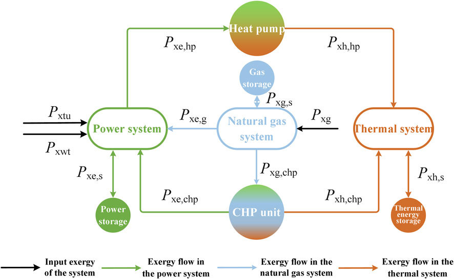
FIGURE 1. IES exergy flow distribution diagram. (P_xg, P_xtu, and P_xwt represent the exergy flows of natural gas, thermal power units, and wind turbines that input the system. P_xe,s, P_xe,chp, and P_xe,hp refer to the exergy flows between the power system and the power storage, the CHP unit, and the heat pump. P_xg,s, P_xe,g, and P_xg,chp are the exergy flows between the natural gas system and the gas storage, the power system, and the CHP unit. P_xh,s, P_xe,hp, and P_xh,chp are the exergy flows between the thermal system and the thermal energy storage, the heat pump, and the CHP unit.)

2.1 Exergy analysis model of power system

The essence of electric conduction is the directional movement of electrons in metals. The intensity and extension variables are electric potential and current during the conduction process. In the power network, electric exergy indicates the ability of electric charges to make useful work under an electric field. Generally, the ground is taken as the zero potential point and the static state value of the potential is U₀ = 0. Electric energy is the highest grade energy that can be completely converted into work. Its energy quality coefficient is equal to 1. Therefore, the change in electric exergy is equal to the change in electric energy, and the active power flow of the power system is the exergy flow, and the active power loss is the exergy loss. This is shown in the following formula:

$\left\{\begin{array}{l}\Delta P_{xe}=\Delta P_e\\ P_{xej}=P_{xei}-{\mathrm{R}}_e{\left(\frac{P_{xei}}{U_i}\right)}^2,\end{array}\right.(3)$

where subscripts i and j represent the beginning and end of the transmission line, respectively. ΔP_xe and ΔP_e refer to the loss of electric exergy and energy, respectively.

In the case of a given initial value ($I=\frac{P_i}{U_i}$), according to the measured data or power flow calculation of the power system, the active power flow distribution and active power loss can be obtained, and then, the exergy flow and exergy loss in the transmission line can be determined.

2.2 Exergy analysis model of thermal system

The thermal network uses hot water as the transmission medium and realizes the transmission of thermal energy by adjusting the temperature between the supply and return pipes. The thermal energy of hot water at temperature T can be expressed as

$P_h=c_p{\rho }_h{\phi }_h\left(T-T_0\right),(4)$

where c_p, ρ_h, and φ_h are the specific thermal capacity, density, and volume flow rates of water, respectively. T₀ is the ambient temperature (25 °C), regarded as the temperature static state value, and T represents the hot water temperature.

The formula for calculating the energy quality coefficient of hot water is as follows:

$\left\{\begin{array}{c}{\lambda }_h=1-\frac{T_0}{T}\mathrm{c}\mathrm{o}\mathrm{n}\mathrm{s}\mathrm{t}\mathrm{a}\mathrm{n}\mathrm{t}\mathrm{t}\mathrm{e}\mathrm{m}\mathrm{p}\mathrm{e}\mathrm{r}\mathrm{a}\mathrm{t}\mathrm{u}\mathrm{r}\mathrm{e}\\ {\lambda }_h=1-\frac{T_0}{T_i-T_j}In\frac{T_i}{T_j}\mathrm{v}\mathrm{a}\mathrm{r}\mathrm{i}\mathrm{a}\mathrm{b}\mathrm{l}\mathrm{e}\mathrm{t}\mathrm{e}\mathrm{m}\mathrm{p}\mathrm{e}\mathrm{r}\mathrm{a}\mathrm{t}\mathrm{u}\mathrm{r}\mathrm{e}\end{array}\right..(5)$

The exergy flow of thermal energy (P_xh) can be expressed as the product of the energy quality coefficient of hot water (λ_h) and the thermal flow (P_h). The calculation of the exergy loss of the thermal system adopts the temperature–entropy model (Chen, 2021). That is, the exergy loss is equal to the sum of the thermal energy loss and entropy increase during the transmission process:

$\Delta P_{xh}=\Delta P_h+T_0\Delta S=c\rho {\phi }_h\left(T_i-T_j+T_{0}In\frac{T_i}{T_j}\right),(6)$

where ΔP_xh and ΔP_h represent the thermal exergy and thermal energy losses during the transmission process, respectively. ΔS refers to the entropy increase in the thermal transfer process.

The entropy increase is calculated as follows:

$\Delta S=c\rho {\phi }_{h}In\frac{T_i}{T_j}.(7)$

2.3 Exergy analysis model of natural gas system

Natural gas is the medium through which energy is transmitted in the natural gas network. Natural gas energy is calculated from the volume flow rates and total calorific value by

$P_g=\frac{1000}{3600}W{\phi }_g,(8)$

where P_g and φ_g represent the energy and volume flow rates of natural gas, respectively. W refers to the low calorific value of natural gas.

The exergy flow of natural gas (P_xg) can be expressed as the product of the energy quality coefficient of natural gas (λ_g) and value of natural gas energy (P_g). Natural gas flows under the impetus of air pressure, and the basic intensive variable related to pressure energy is air pressure. The static state value of air pressure is 0.1 Mpa, the basic extensive variable is volume, and the flux of the basic extensive variable is volume flow rate. The exergy losses are generated during the flow of natural gas, which includes the internal pressure exergy loss of the pipeline and chemical exergy loss of the input natural gas, and the exergy loss is calculated as follows:

$\Delta P_{\mathrm{x}\mathrm{g}}={\displaystyle \sum _{l_g=1}^{N_{{\mathrm{l}}_{\mathrm{g}}}}}\Delta P_{xng}^{l_g}+{\displaystyle \sum _{m_g=1}^{N_{m_g}}}{P}_{xog}^{m_g}(9)$

where ΔP_xg is the total exergy loss in the natural gas network, l_g represents the number of network pipelines, N_lg is the total number of gas network pipelines, ΔP_xng^lg refers to the internal pressure exergy loss of the pipeline, m_g is the number of gas sources, N_mg represents the total number of gas sources, and the external pressure consumption of gas source m_g is P_xog^mg.

$\Delta P_{xng}={\phi }_g\left({\pi }_i-{\pi }_j\right),(10)$

$P_{xog}^{m_g}=\left(1-{\lambda }_g\right)P_g,(11)$

where π_i and π_j represent the pressure at nodes i and j, respectively.

The outlet pressure of the pipeline is calculated as follows:

${\pi }_j=\sqrt{{\pi }_i-1.27\times {10}^7\gamma \frac{{\phi }_g^2}{D^5}{\rho }_g\frac{T_g}{T_0}L},(12)$

where γ represents the coefficient of hydraulic friction. ρ_g refers to the density of natural gas. D, T_g, and L are the diameter, temperature, and length of the natural gas pipeline, respectively.

2.4 Exergy analysis model of CHP units

CHP units use natural gas as fuel, converted into two forms of energy (electricity and thermal energy). The process energy quality changes to achieve the cascade utilization of energy. The units’ exergy loss includes natural gas chemical energy loss and internal exergy loss. Combined with such as the unit’s power generation efficiency and thermoelectric ratio, the exergy loss during the energy conversion process can be obtained (Chen et al., 2020), and the expression is as follows:

$\Delta P_{xchp}={\displaystyle \sum _{s=1}^{N_s}}\left(\Delta P_{xnchp}^s+\Delta P_{xochp}^s\right)={\displaystyle \sum _{s=1}^{N_s}}\left(P_{xgchp}^s-P_{xechp}^s-P_{xhchp}^s+P_{xog}^s\right),(13)$

where ΔP_xchp represents the total exergy loss of the CHP unit, P_xnchp refers to the internal exergy loss, which is equal to the sum of the input natural gas fuel chemistry exergy P_xgchp^s minus the output electricity exergy P_xechp^s and the thermal exergy P_xhchp^s. ΔP_xochp is the external exergy loss, which is equal to the chemical exergy loss of natural gas. s is the number of CHP units, and N_s is the total number of CHP units.

The thermal output value of a CHP unit can be expressed as follows:

$P_{h,chp}=k^{chp}\cdot P_{e,chp},(14)$

where P_h,chp and P_e,chp refer to the CHP unit’s thermal and electric output value, and k^chp is the thermoelectric ratio of the CHP unit.

The consumption of natural gas in the CHP unit can be expressed as

$P_{\mathrm{g},chp}=\frac{P_{h,chp}}{k^{chp}{\eta }_{chp}}.(15)$

where η_chp represents the efficiency of power generation.

3 Adjustable flexibility capacity of IES based on exergy analysis model

Through the exergy analysis models explained in Section 2, the exergy flow and exergy loss at each moment can be obtained. On this basis, this section considers the dynamic characteristics of the gas–thermal pipeline network, analyzes the useful energy stored in the pipeline according to the energy quality coefficients of natural gas and thermal energy, analyzes the flexibility capacity of each subsystem, and effectively uses the various available energy sources of the system.

3.1 Flexibility supply model of power system

In the power system, conventional thermal power units are considered to provide flexibility, which is related to the units’ current operating state and ramp rates. The units can provide upward flexibility if there is room for increasing output. While there is room for reducing output, the units can provide downward flexibility. Therefore, the upward and downward flexibility provided by the power system can be represented as

$\left\{\begin{array}{l}{F}_{e,t}^{up}={\displaystyle \sum }_{tu\in {\mathrm{\Omega }}_{tu}}\min ({\delta }_{tu,t}{r}_{tu,t}^{up}\Delta t,{\delta }_{tu,t}{P}_{tu}^{\max }-P_{tu,t})\\ F_{e,t}^{dn}={\displaystyle \sum }_{tu\in {\mathrm{\Omega }}_{tu}}\min ({\delta }_{tu,t}{r}_{tu,t}^{dn}\Delta t,P_{tu,t}-{\delta }_{tu,t}{P}_{tu}^{\min })\end{array}\right.,(16)$

where r_tu,t^up and r_tu,t^dn are the uphill and downhill ramp rates of thermal power unit tu at time t. P_tu,t is the output value of unit tu at time t. P_tu,t^max and P_tu,t^min are the upper and lower limits of the active output of unit tu, respectively. Δt is the scheduling time interval. δ_tu,t is the 0–1 variable representing the start–stop state of unit tu at time t. Ω_tu represents a collection of thermal power units.

3.2 Flexibility supply model of heating system

3.2.1 Modeling of heating system dynamics

The heating system can be divided into a transmission system composed of a primary pipe network and a distribution system composed of a secondary pipe network, with heat exchange being achieved through heat exchange stations. Among these, the transmission delay of thermal energy and the virtual heat storage characteristics of the heat network are mainly reflected in the primary heat network. Virtual energy storage in the heat network has to consider factors such as pipeline temperature drop and transmission delay. This section combines the quasi-dynamic characteristics of thermal energy transport and models it using the nodal method (Wang et al., 2020).

In each scheduling period Δt, the transmission delay t_hl of the thermal pipeline is between t₁ and t₂, assuming t₁ = (k − 1)Δt, t₂ = kΔt, then the outlet temperature of pipeline hl at time t is calculated as follows:

$T_{hl,t}^{out}=C_1{C}_3{T}_{hl,t-t_1}^{out}+C_2{C}_4{T}_{hl,t-t_2}^{out}+\left(1-C_1{C}_3-C_2{C}_4\right)T^{am},(17)$

where T_hl,Δt-t1^out and T_hl,Δt-t2^out represent the water temperature at the entrance of the pipeline at times Δt–t₁ and Δt–t₂, respectively. T^am is the ambient temperature around the pipe. C₁, C₂, C₃, and C₄ are constants.

The quasi-dynamic temperature characteristics of the pipes in the heating network are modeled as virtual heat storage characteristics, calculated as follows:

$H_t={\displaystyle \sum }_{hl\in {\mathrm{\Omega }}_{hl}}{c}_p\rho [{\phi }_h^{su}\left(T_{hl,out}^{t,su}-T_{hl,in}^{t,su}\right)+{\phi }_h^{re}\left(T_{hl,out}^{t,re}-T_{hl,in}^{t,re}\right)],(18)$

where H_t is the virtual heating energy storage of the heat network at time t. φ_h^su and φ_h^re represent the volume flow rates of hot water flowing through the supply and return pipes hl at time t, respectively. H_t > 0 refers to heat storage, and H_t ≤ 0 represents heat release.

3.2.2 Flexibility supply model of heating system

Considering the output limit, ramp rates of CHP units, dynamic characteristics of the heat network, and energy quality coefficient of hot water, the flexibility supplied by the heat network can be further expressed as

$\left\{\begin{array}{l}{F}_{h,t}^{up}=\min \left\{\left.{\displaystyle \sum }_{chp\in \mathrm{\Omega }chp}\left(P_{chp}^{\max }-P_{chp,t}\right),{\displaystyle \sum }_{chp\in \mathrm{\Omega }chp}{r}_{chp,t}^{up}\Delta t,{\lambda }_h{H}_{sp,t}\right)\right\}\\ F_{h,t}^{dn}=\min \left\{\left.{\displaystyle \sum }_{chp\in \mathrm{\Omega }chp}\left(P_{chp,t}-P_{chp}^{\min }\right),{\displaystyle \sum }_{chp\in \mathrm{\Omega }chp}{r}_{chp,t}^{dn}\Delta t,{\lambda }_h{H}_{rp,t}\right)\right\}\end{array}\right.,(19)$

where r_chp,t^up and r_chp,t^dn are the uphill and downhill ramp rates of CHP unit chp at t moment. P_chp,t is the output value of the unit chp at t moment. P_chp^max and P_chp^min represent the upper and lower limits of the active output of unit chp, respectively. H_sp,t and H_rp,t refer to the heat storage and heat release of the heating network at time t, respectively. Ω_chp is a collection of CHP units.

3.3 Flexibility supply model of natural gas system

3.3.1 Modeling of natural gas system dynamics

Natural gas is slow and compressive that the pipeline’s storage space can store it, providing upward flexibility by releasing natural gas and increasing the amount of gas available to gas turbines. Downward flexibility can be provided by storing natural gas and reducing the available amount of gas to gas turbines. The ability to provide operational flexibility in real time for the natural gas system is closely related to the linepack state and constrained by volume flow rates of gas, the upper and lower limits of pressure, etc.

The model of the gas network linepack in this work adopts dynamic modeling, and the mathematical model is expressed as

$M_{gl}^t=M_{gl}^{t-1}+G_{gl,t}^{in}-G_{gl,t}^{out},(20)$

where M_gl^t is the natural gas linepack at time t.

The initial linepack M_gl,tini is

$M_{gl.t_{ini}}=\frac{pi\times L{D}_{gl}^2{\pi }_{gl,t}^{av}}{4R_g{T}_{g}Z{\rho }_g},(21)$

where π_gl,t^av = (π_i+π_j)/2.

${\overline{G}}_{gl,t}\left|{\overline{G}}_{gl,t}\right|={\left(\frac{pi}{4}\right)}^2\frac{D^5}{L\gamma R{T}_{g}Z{\rho }_g^2}\left({\pi }_i^2-{\pi }_j^2\right),(22)$

${\overline{G}}_{gl}^{\min }\le {\overline{G}}_{gl,t}\le {\overline{G}}_{gl}^{\max },(23)$

where ${\overline{G}}_{gl,t}=\left(G_{gl,t}^{in}+G_{gl,t}^{out}\right)/2$.

3.3.2 Modeling of flexibility supply in natural gas system

Considering the ramp rates, output limits, dynamic characteristics of gas pipelines, and energy quality coefficient of natural gas, the flexibility supplied by the natural gas system can be further expressed as

$\left\{\begin{array}{l}{F}_{g,t}^{up}=\min \left({\displaystyle \sum }_{gt\in {\mathrm{\Omega }}_{gt}}\left(P_{gt}^{\max }-P_{gt,t}\right),{\displaystyle \sum }_{gt\in {\mathrm{\Omega }}_{gt}}{r}_{gt,t}^{up}\Delta t,{\lambda }_g{G}_{rp,t}\right)\\ F_{g,t}^{dn}=\min \left({\displaystyle \sum }_{gt\in {\mathrm{\Omega }}_{gt}}\left(P_{gt,t}-P_{gt}^{\min }\right),{\displaystyle \sum }_{gt\in {\mathrm{\Omega }}_{gt}}{r}_{gt,t}^{dn}\Delta t,{\lambda }_g{G}_{sp,t}\right)\end{array}\right.,(24)$

where r_gt,t^up and r_gt,t^dn are the uphill and downhill ramp rates of the gas turbine gt at time t, respectively. P_gt,t is the output value of unit gt at time t. P_gt^max and P_gt^min represent the upper and lower limits of the active output of unit gt, respectively. G_rp,t and G_sp,t refer to the storage and release of natural gas power in the gas pipeline at time t, respectively. Ω_gt is a collection of gas turbine units.

3.3.3 IES flexibility requirements model

The flexibility requirements of the system at a particular moment are related to the change in the net load of the scheduling time and the limit value of the system’s flexibility requirements (Zhang et al., 2018), which can be expressed as

$\left\{\begin{array}{l}{F}_{d,t}^{up}=F_{\lim ,t}^{up}-\left(P_{load,t+1}-P_{load,t}\right)\\ F_{d,t}^{dn}=F_{\lim ,t}^{dn}-\left(P_{load,t}-P_{load,t+1}\right)\end{array}\right.,(25)$

where F_d,t^up and F_d,t^dn are the upward and downward flexibility demands of time t, respectively. F_lim,t^up and F_lim,t^dn refer to the upper and lower flexibility demands of the system at time t, respectively. P_load,t represents the load at time t.

4 IES's flexible operation optimization model based on exergy analysis

The characteristics of the gas network linepack and delay characteristics of pipelines in the thermal system can provide resources for the operational flexibility of the system. Based on the adjustable flexibility capacity model of the IES under the exergy analysis constructed in Section 3, the IES optimization operation model considering the dynamic characteristics of the network is constructed.

4.1 Objective function

The optimization operation model of the electricity–gas–thermal IES is established to minimize the sum of the energy purchase cost, wind curtailment penalty cost, and compensation cost of flexibility resource mobilization.

$\min C=C_{ep}+C_{wp}-C_{fm},(26)$

where C_ep represents the energy purchase cost, C_wp is the wind curtailment penalty cost, and C_fm compensates for the compensation cost of flexibility resource mobilization.

The energy purchase cost is as follows:

$C_{ep}=C_{pe}+C_{pg},(27)$

where C_pe and C_pg refer to the cost of purchasing electricity from the external grid and natural gas, respectively.

The curtailment penalty cost is as follows:

$C_{wp}={\displaystyle \sum _{t=1}^{t_{end}}}{c}_{wt}\left(P_{wt}-P_{wt,t}\right)\cdot \Delta T,(28)$

where c_wt is the penalty cost factor for wind power. P_wt refers to the outputs of wind turbines.

The compensation cost of flexibility in resource mobilization is expressed as follows:

$C_{fm}={\displaystyle \sum _{t=1}^{t_{end}}}{\displaystyle \sum }_{f\in {\mathrm{\Omega }}_F}{r}_{f,t}{F}_{f,t}\Delta T,(29)$

where r_f,t and F_f,t represent the unit adjustment compensation cost and capacity of the flexibility resource f at time t, respectively.

4.2 Constraints

4.2.1 Power system constraints

(1) Power balance constraints

${\displaystyle \sum }_{tu\in a}{P}_{tu,t}+{\displaystyle \sum }_{chp\in a}{P}_{chp,t}+{\displaystyle \sum }_{gt\in a}{P}_{gt,t}+{\displaystyle \sum }_{wt\in a}{P}_{wt,t}=P_{a,t}^{load}+{\displaystyle \sum }_{b\in a}{P}_{ab,t},(30)$

where P_wt,t, P_a,t^load, and P_ab,t refer to the output of wind turbines, electrical load of node a, and power of the line connected to node a at time t, respectively. tu $\in$ a indicates that the thermal power unit u is connected to the power node a, and the other descriptions are the same as mentioned above.

(2) Unit output constraints

The output limit of thermal power units can be expressed as

${\delta }_{tu,t}\cdot P_{tu}^{\min }\le P_{tu,t}\le {\delta }_{tu,t}\cdot P_{tu}^{\mathrm{m}ax}.(31)$

(3) Ramp constraints

The ramp rate constraints of thermal power units can be expressed as

$\left|P_{tu}\left(t+1\right)-P_{tu}\left(t\right)\right|\le \Delta r_{tu},(32)$

where Δr_tu represents the ramp power of the thermal power unit.

4.2.2 Thermal system constraints

(1) Thermal network constraints

According to Kirchhoff’s law, the sum of the mass flows flowing into and out of the thermal energy load node is equal.

${\displaystyle \sum }_{hl\in {\mathrm{\Omega }}_{hl}^{in}}{Q}_{hl,t}={\displaystyle \sum }_{hl\in {\mathrm{\Omega }}_{hl}^{out}}{Q}_{hl,t},(33)$

where Q_hl,t represents the mass flow of hot water flowing through the pipeline hl at time t, and Ω_hlⁱⁿ and Ω_hl^out represent the collection of pipelines flowing from the pipeline to node a and from node a to the pipeline, respectively.

The limits of mass flow are as follows:

$Q_{hl,t}^{\min }\le Q_{hl,t}\le Q_{hl,t}^{\max },(34)$

where Q_hl,t^min and Q_hl,t^max represent the minimum and maximum mass flow rates of pipeline hl at time t.

(2) CHP unit constraints

The electrical and thermal output limits of a CHP unit can be expressed as follows:

$\left\{\begin{array}{l}{P}_{e,chp}^{\min }\le P_{e,chp}\le P_{e,chp}^{\max }\\ P_{h,chp}^{\min }\le P_{h,chp}\le P_{e,chp}^{\max }\end{array}\right.,(35)$

where P_e,chp^min and P_e,chp^max represent the minimum and maximum electrical outputs, respectively, while P_h,chp^min and P_h,chp^max refer to the minimum and maximum thermal outputs, respectively.

(3) Ramp constraints

The ramp constraints of a CHP unit can be expressed as follows:

$\left|P_{e,chp}\left(t+1\right)-P_{e,chp}\left(t\right)\right|\le \Delta r_{chp},(36)$

where Δr_chp represents the ramp power of the CHP unit.

4.2.3 Natural gas system constraints

(1) Pipeline flow balancing constraints

${\displaystyle \sum }_{m_g\in {\mathrm{\Omega }}_{m_g}}{G}_{g,t}+{\displaystyle \sum }_{gl\in {\mathrm{\Omega }}_{gl}}\left(G_{gl,t}^{out}-G_{gl,t}^{in}\right)-G_{d,t}={\displaystyle \sum }_{gl\in {\mathrm{\Omega }}_{gl}}{G}_{gl,t},(37)$

where G_g,t represents the gas production of the gas source at time t. G_gl,tⁱⁿ and G_gl,t^out are the inflow and outflow of gas in the pipeline gl at time t, respectively. G_d,t and G_gl,t refer to the gas demand and the amount of gas flowing through the pipeline gl at time t, respectively.

(2) Gas transmission capacity constraints

$G_{gl}^{\min }\le G_{gl,t}\le G_{gl}^{\max },(38)$

where G_gl^min and G_gl^max are the upper and lower limits of the allowable gas transmission volume of the gas pipeline, respectively.

(3) Linepack constraints

$M_{gl}^{\min }\le M_{gl,t}\le M_{gl}^{\max },(39)$

where M_gl^min and M_gl^max represent the lower and upper limits of the gas network linepack.

4.2.4 Natural gas system constraints

The flowchart of the overall solving process of the optimization model is summarized in Figure 2, which first establishes an optimized operation model and then linearizes quadratic terms that are difficult to calculate directly in the model, solving the model by considering economic and environmental benefits, and operational flexibility.

FIGURE 2

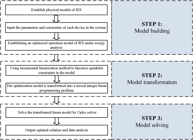
FIGURE 2. Model solving process.

4.2.5 Linearization method of quadratic constraints

The non-linear equations existing in the proposed model are Equations 12, 22. The non-linear factors are the squared volume flow rates (φ_g²), squared pressures (π_i², π_j²), and squared average gas flow (${\overline{G}}_{gl,t}^2$). It is hard to solve them directly and takes a long time, so we adopt the incremental linearization method with quadratic constraints to linearize them separately. Considering that Equations 16, 19, and 22 are expressions of type X = min (Y, Z), they can be transformed into two terms: X ≤ Y and X ≤ Z, thereby transforming the model into a mixed integer linear programming problem. The specific process of incremental linearization is detailed in the study by Chen et al. (2020).

5 Case study

5.1 Basic data

This work uses the YALMIP toolbox for modeling and employs CPLEX 12.8 in MATLAB R2018b to solve the model. The system comprises an IEEE 39-node power system, a 6-node thermal system, and a 20-node natural gas system in Belgium. The IEEE 39-node power subsystem data are taken from the sample data in the MATPOWER toolkit, which possesses 10 generator sets: six thermal power units, one CHP unit, two gas turbine units, and one wind turbine, with a total capacity of 6,627 MW. The natural gas system contains six gas sources and nine gas loads comprised of seven conventional gas loads and two gas turbine generator loads. The thermal system includes one CHP unit, three thermal energy loads, and five thermal pipelines. The scheduling cycle and interval are 24 h and 1 h, respectively. This work compares and analyzes the following four scenarios to determine the influence of IES network dynamics on the operation economy:

Scenario 1: the dynamic characteristics of the gas–thermal network are not considered for energy analysis.

Scenario 2: the dynamic characteristics of the gas–thermal network are considered for energy analysis.

Scenario 3: the dynamic characteristics of the gas–thermal network are not considered for exergy analysis.

Scenario 4: the dynamic characteristics of the gas–thermal network are considered for exergy analysis.

5.2 Analysis of dynamic characteristics of gas–thermal pipe network

Table 1 outlines the details of the total cost, energy purchase cost, and compensation cost of flexibility resource mobilization in the four different scenarios. As summarized in Table 1, considering dynamic characteristics in the system can promote wind power consumption, improve environmental benefits, and reduce total cost. Scenario 2 has an increase of 5.81% in wind power output when compared to Scenario 1, an increase of 52.53% in compensation cost for flexibility resources, and a reduction of 2.54% in total cost. In comparison with Scenario 3, the wind power output of Scenario 4 is increased by 12.12%, the compensation cost for flexibility resources is increased by 42.71%, while the total cost is reduced by 2.20%. Scenario 2 has 1.38% higher utilization rate of wind power, 6.88% more flexibility resources, and 0.58% lower total cost than Scenario 4. From the energy perspective, the system exhibits better performance, but the energy stored in pipes has a different “quality,” so the analysis cannot characterize the actual available energy. The exergy analysis can consider the “quantity” and “quality” of energy and better reflect the energy utilization in the system, and the evaluation results are more reasonable.

TABLE 1

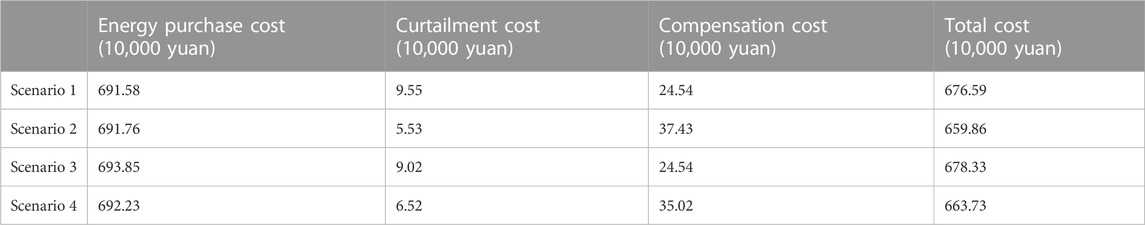
TABLE 1. Optimization results in different scenarios.

5.3 Distribution of energy and exergy losses in IES

This section analyzes the exergy losses of each subsystem in the electrical–gas–thermal IES within 24 h (shown in Figures 3, 4, 5, 6) and the value and proportion of energy and exergy losses (shown in Table 2).

FIGURE 3

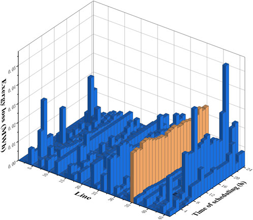
FIGURE 3. Exergy loss in the power system.

FIGURE 4

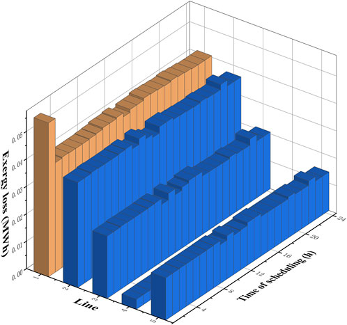
FIGURE 4. Exergy loss in the thermal system.

FIGURE 5

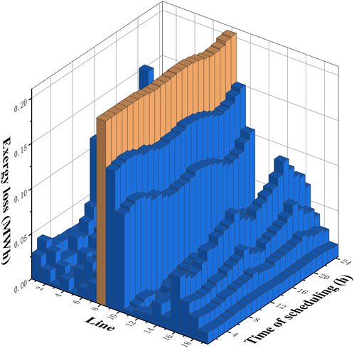
FIGURE 5. Exergy loss in the natural gas system.

FIGURE 6

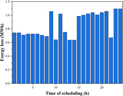
FIGURE 6. Exergy loss in CHP.

TABLE 2

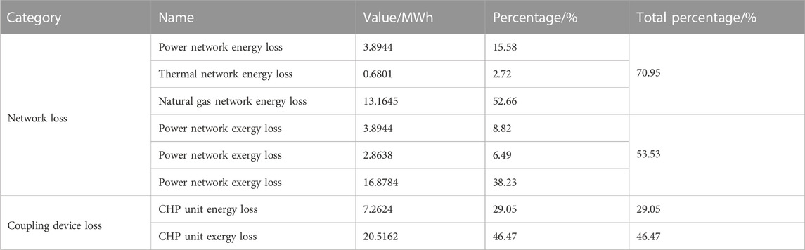
TABLE 2. Energy loss and exergy loss distribution data of the electricity–gas–thermal IES.

From Figures 3, 4, 5, in the power system, the total exergy loss of the 35th transmission line in 24 h is the largest, which is 0.6020 MWh, accounting for 15.46% of the total exergy loss. At the 21st hour, the exergy loss of the 44th transmission line is the largest at 0.0560 MWh. In the thermal system, the total exergy loss of the 1st hot water pipeline in 24 h is the largest at 0.9927 MWh, accounting for 34.47% of the total exergy loss, and reaches its maximum at 0.0560 MWh in the 15th hour. In the natural gas system, the total exergy loss of the 8th pipeline in 24 h is the largest at 4.8784 MWh, accounting for 23.12% of the total exergy loss, and reaches its maximum at 0.2048 MWh in the 6th hour.

According to the topology of the IES network, the initial node of the 1st pipeline in the thermal system is connected to the CHP unit, and the initial node of the 8th pipeline in the natural gas system is connected to the gas source, which indicates that the energy input will affect the exergy loss of the line directly connected to it. As seen from Figure 6, the maximum exergy loss value of the CHP unit appeared in the 24th hour, reaching 1.0940 MWh, accounting for 5.33% of the total exergy loss of the unit. According to the exergy analysis model, the exergy flow and exergy loss distribution of all pipelines and equipment in the system can be calculated and analyzed such that relevant staff can grasp the system’s real-time energy consumption and make timely adjustments.

Table 2 demonstrates that the CHP unit has the highest exergy loss, followed by gas, power, and thermal systems. The exergy loss in the network accounts for about half of the total exergy loss, accounting for 57.59%, of which the exergy loss of the natural gas network accounts for 71.41%. This work only considers the coupling device of the CHP units, which accounts for 46.47% of the total exergy loss. From the energy perspective, the natural gas network has the highest energy loss, followed by the CHP unit, power, and thermal systems. Energy loss in the network accounts for more than 70% of the system’s energy loss, reaching 70.95%, with over half of the energy loss occurring in natural gas networks. The energy loss of the CHP unit is 7.2624 MWh, accounting for 29.05% of the total energy loss. Both from the point of view of the energy and exergy analysis, the loss of natural gas in the network is significant. However, the CHP unit’s energy and exergy losses are quite different. When there are three energy forms of electricity, gas, and thermal simultaneously, the calculation results of the energy loss become easily misleading due to their different “qualities.” The exergy analysis can consider the “quantity” and “quality” of different energies, better reflect the loss of useful energy during the energy conversion process, and make the evaluation results more reasonable. Therefore, in the system optimization process, the focus should be on reducing the loss of the CHP units. Further analysis of the CHP unit’s internal and external losses is shown in Table 3.

TABLE 3

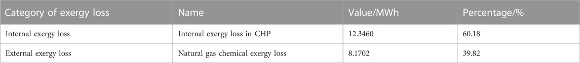
TABLE 3. Exergy loss data in CHP.

The exergy loss generated by the CHP unit in the energy supply process can be divided into irreversible exergy loss caused by the internal energy conversion process and external natural gas chemical exergy loss. As can be seen from Table 3, the internal exergy loss is 12.3460 MWh, accounting for 60.18%, while the external exergy loss is 8.1702 MWh, accounting for 39.82%. From Equations 14 and 15, it is seen that the ambient temperature, CHP unit thermoelectric ratio, and power generation efficiency are key factors affecting the exergy loss. When the ambient temperature remains constant, the chemical energy and energy quality coefficient of natural gas remain unchanged, and the external loss of the CHP unit is proportional to the natural gas consumed by the unit for power generation. The more natural gas the unit consumes, the greater is its external exergy loss. To reduce the exergy loss of the unit, a unit with a suitable thermoelectric ratio and power generation efficiency should be selected so that the unit consumes less natural gas, has a larger output of electrical and thermal energy, and where the internal and external exergy losses are more diminutive.

5.4 Flexibility provided by system under exergy analysis

To analyze the impact of the network dynamic characteristics on IES’s flexibility under exergy analysis, this work calculates the upward and downward flexibility capacities of IES supply for each period under the upper and lower flexibility demand limits of 200 MW. As shown in Figures 7, 8, the lines indicate the flexibility demands of the system under the limits. The flexibility demands of the system at different times are related to the electrical loads and the fluctuation in wind power outputs, so the flexibility demands at different times vary considerably.

FIGURE 7

FIGURE 7. Upward flexibility provided by the system under exergy analysis.

FIGURE 8

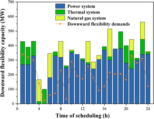
FIGURE 8. Downward flexibility provided by the system under exergy analysis.

Figures 7, 8 reveal that the flexibility supplied by the gas–thermal system varies with time due to the energy consumption characteristics of the gas–thermal load and the constraints of the gas–thermal pipe network. In the 1st–7th hour and 21st–24th hour, the output of wind power shows significant fluctuation, and the flexibility demand of the system is enormous. The conventional thermal power units in the power system cannot meet the rapidly changing loads. However, at this time, the flexibility supply is greater than the flexibility demand, which indicates that considering the dynamic characteristics of the gas–thermal pipeline network, the coordinated dispatch of the gas–thermal system can provide sufficient flexibility.

As depicted in Figure 9, under exergy analysis, when the dynamic characteristics of the gas–thermal pipeline network are taken into account, wind curtailment rates of the system decrease from 11.22% to 8.27%, which means that considering the dynamic characteristics of the gas–thermal pipe network, the system can provide more flexibility capacity to effectively respond to external load changes and reduce wind abandonment.

FIGURE 9

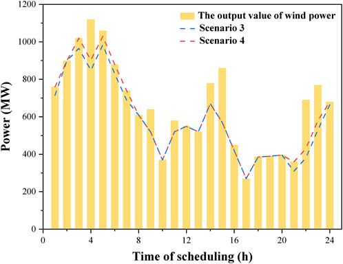
FIGURE 9. Wind power consumption.

6 Conclusion

Based on the energy network theory, this work establishes an integrated electricity–gas–thermal energy system analysis model, derives the mathematical expression of the flexibility capacity of the system's supply based on the dynamic characteristics of the gas–thermal pipe network, and establishes the flexible operation optimization model of the IES. The performance of the system in terms of economy, wind curtailment, and flexibility in different scenarios was analyzed, the influence of energy storage characteristics of the gas–thermal pipe network on the optimization results was studied, and the following conclusions were obtained.

(1) Exergy analysis, analyzing the “quantity” and “quality” of different forms of energy, provides a more objective method for evaluating the energy utilization degree of the IES.

(2) Less energy loss and greater exergy loss are observed in coupling equipment (CHP unit) by calculating and analyzing the energy and exergy loss distribution of all pipelines and equipment in the system. It suggests that the exergy analysis can better reflect the loss in the energy conversion process and identify the critical links to improve the energy-saving potential of the IES.

(3) By utilizing the dynamic characteristics of the gas–thermal pipeline network, wind power can be absorbed as storage energy during windy periods and released during windless periods.

This article considers the dynamic characteristics of the gas–thermal pipeline, even as the energy losses generated by thermal energy and natural gas during transmission cannot be ignored. These losses are equivalent to increasing gas and thermal loads of the system, which in turn increase the CHP unit’s thermal output. Due to its thermoelectric solid coupling characteristics, its electrical output also increases, which may occupy the grid connection space of wind power and trigger new renewable energy consumption problems. Therefore, exploring the dynamic characteristics of the gas–thermal pipeline network and its subsequent changes is still necessary. The comprehensive optimization operation model of the IES based on exergy analysis and dynamic characteristics proposed in this article has not established a unified exergy efficiency calculation model. Using exergy efficiency, we can analyze the impact of different equipment types and operating parameters on energy utilization levels and identify key energy-saving links. Further related research is necessary to explore the complementary characteristics of the IES and improve the flexibility and economy of the system.

Data availability statement

The original contributions presented in the study are included in the article/supplementary material; further inquiries can be directed to the corresponding author.

Author contributions

XL, TW, and SL contributed to the conceptualization. XL and TW built the model. TW was responsible for the software. XL and TW visualized the results and wrote the original draft of the manuscript. XL and TW reviewed and edited the manuscript. XL supervised the research and managed the project. Access to funding was provided by XL and SL. All authors contributed to the article and approved the submitted version.

Funding

This work is supported by the National Natural Science Foundation of China (No. 51977127).

Conflict of interest

The authors declare that the research was conducted in the absence of any commercial or financial relationships that could be construed as a potential conflict of interest.

Publisher’s note

All claims expressed in this article are solely those of the authors and do not necessarily represent those of their affiliated organizations, or those of the publisher, editors, and reviewers. Any product that may be evaluated in this article, or claim that may be made by its manufacturer, is not guaranteed or endorsed by the publisher.

References

Abdin, A. F., and Zio, E. (2018). An integrated framework for operational flexibility assessment in multi-period power system planning with renewable energy production. Appl. Energy 222, 898–914. doi:10.1016/j.apenergy.2018.04.009

CrossRef Full Text | Google Scholar

Alabi, T. M., Agbajor, F. D., Yang, Z., Lu, L., and Ogungbile, A. J. (2022). Strategic potential of multi-energy system towards carbon neutrality: A forward-looking overview[J]. Energy and Built Environment 4 (6), 689–708. doi:10.1016/j.enbenv.2022.06.007

CrossRef Full Text | Google Scholar

Berjawi, A. E. H., Walker, S. L., Patsios, C., and Hosseini, S. H. R. (2021). An evaluation framework for future integrated energy systems: A whole energy systems approach. Renew. Sustain. Energy Rev. 145, 111163. doi:10.1016/j.rser.2021.111163

CrossRef Full Text | Google Scholar

Bie, C., Ren, Y., and Li, G. (2022). Morphological structure and development path of urban energy systems for carbon emission peak and carbon neutrality[J]. Autom. Electr. Power Syst. 46 (17), 3–15. doi:10.7500/AEPS20220601006

CrossRef Full Text | Google Scholar

Chen, H., Chen, S., Li, M., and Chen, J. (2020). Optimal operation of integrated energy system based on exergy analysis and adaptive genetic algorithm. IEEE Access 8, 158752–158764. doi:10.1109/ACCESS.2020.3018587

CrossRef Full Text | Google Scholar

Chen, H., Weijun, C., and Jianrun, C. (2021). Power internet of things technology with energy and information fusion[J]. Power Syst. Prot. control. 49 (22), 8–17. doi:10.19783/j.cnki.pspc.202163

CrossRef Full Text | Google Scholar

Chen, M., Lu, H., Chang, X., and Liao, H. (2023). An optimization on an integrated energy system of combined heat and power, carbon capture system and power to gas by considering flexible load. Energy 273, 127203. doi:10.1016/j.energy.2023.127203

CrossRef Full Text | Google Scholar

Chen, S. (2021). Dynamic evolution analysis and operation optimization of exergy in integrated energy system based on energy network theory[D]. Guangzhou: South China University of technology, 85.

Google Scholar

Chen, X., Wang, C., Wu, Q., Dong, X., Yang, M., He, S., et al. (2020). Optimal operation of integrated energy system considering dynamic heat-gas characteristics and uncertain wind power. Energy 198, 117270. doi:10.1016/j.energy.2020.117270

CrossRef Full Text | Google Scholar

Chen, Y., Sun, H., and Guo, Q. (2020). Energy curcuit theory of integrated energy system analysis (V): Integrated electricity-heat-gas dispatch[J]. Proc. CSEE 40 (24), 7928–7937+8230. doi:10.13334/j.0258-8013.pcsee.200028

CrossRef Full Text | Google Scholar

Clegg, S., and Mancarella, P. (2016). Integrated electrical and gas network flexibility assessment in low-carbon multi-energy systems. IEEE Throughput Sustain. Energy 7 (2), 718–731. doi:10.1109/TSTE.2015.2497329

CrossRef Full Text | Google Scholar

Dalala, Z., Al-Omari, M., Al-Addous, M., Bdour, M., Al-Khasawneh, Y., and Alkasrawi, M. (2022). Increased renewable energy penetration in national electrical grids constraints and solutions. Energy. 246, 123361. doi:10.1016/j.energy.2022.123361

CrossRef Full Text | Google Scholar

Ebrahimi, H., Yazdaninejadi, A., and Golshannavaz, S. (2022). Demand response programs in power systems with energy storage system-coordinated wind energy sources: A security-constrained problem. J. Clean. Prod. 335, 130342. doi:10.1016/j.jclepro.2021.130342

CrossRef Full Text | Google Scholar

Fan, W., Tan, Q., Zhang, A., Ju, L., Wang, Y., Yin, Z., et al. (2023). A Bi-level optimization model of integrated energy system considering wind power uncertainty. Renew. Energy 202, 973–991. doi:10.1016/j.renene.2022.12.007

CrossRef Full Text | Google Scholar

Farzaneh-Gord, M., and Rahbari, H. R. (2018). Response of natural gas distribution pipeline networks to ambient temperature variation (unsteady simulation). J. Nat. Gas. Sci. Eng. 52, 94–105. doi:10.1016/j.jngse.2018.01.024

CrossRef Full Text | Google Scholar

Gord, M. F., Roozbahani, M., Rahbari, H. R., and Hosseini, S. J. H. (2013). Modeling thermodynamic properties of natural gas mixtures using perturbed-chain statistical associating fluid theory. 86 (6), 867–878. doi:10.1134/S1070427213060153

PubMed Abstract | CrossRef Full Text | Google Scholar

Hosseini, S. E., Ahmarinejad, A., Tabrizian, M., and Bidgoli, M. A. (2022). Resilience enhancement of integrated electricity-gas-heating networks through automatic switching in the presence of energy storage systems. J. Energy Storage 47, 103662. doi:10.1016/j.est.2021.103662

CrossRef Full Text | Google Scholar

Hu, X., Zhang, H., Chen, D., Li, Y., Wang, L., Zhang, F., et al. (2020). Multi-objective planning for integrated energy systems considering both exergy efficiency and economy. Energy 197, 117155. doi:10.1016/j.energy.2020.117155

CrossRef Full Text | Google Scholar

Li, J., Liu, F., Li, Z., Shao, C., and Liu, X. (2018). Grid-side flexibility of power systems in integrating large-scale renewable generations: A critical review on concepts, formulations and solution approaches. Renew. Sustain. Energy Rev. 93, 272–284. doi:10.1016/j.rser.2018.04.109

CrossRef Full Text | Google Scholar

Li, J., Wang, D., and Jia, H. (2022). Exergy flow mechanism and analysis method for integrated energy systems[J]. Autom. Electr. Power Syst. 46 (12), 163–173. doi:10.7500/AEPS20211029002

CrossRef Full Text | Google Scholar

Li, J., Wang, D., Jia, H., Lei, Y., Zhou, T., and Guo, Y. (2022). Mechanism analysis and unified calculation model of exergy flow distribution in regional integrated energy system. Appl. Energy 324, 119725. doi:10.1016/j.apenergy.2022.119725

CrossRef Full Text | Google Scholar

Li, X., Li, W., Zhang, R., Jiang, T., Chen, H., and Li, G. (2020). Collaborative scheduling and flexibility assessment of integrated electricity and district heating systems utilizing thermal inertia of district heating network and aggregated buildings. Appl. Energy 258, 114021. doi:10.1016/j.apenergy.2019.114021

CrossRef Full Text | Google Scholar

Liu, D., Ma, H., and Wang, B. (2018). Operational optimization of regional integrated energy system with CCHP and energy storage system[J]. Autom. Electr. Power Syst. 42 (04), 113–120+141. doi:10.7500/AEPS20170512002

CrossRef Full Text | Google Scholar

Liu, S., Zhou, C., Guo, H., Shi, Q., Song, T. E., Schomer, I., et al. (2021). Operational optimization of a building-level integrated energy system considering additional potential benefits of energy storage. J]. Prot. Control Mod. Power Syst. 6 (1), 4. doi:10.1186/s41601-021-00184-0

CrossRef Full Text | Google Scholar

Qiu, H., Gu, W., Liu, P., Sun, Q., Wu, Z., and Lu, X. (2022). Application of two-stage robust optimization theory in power system scheduling under uncertainties: A review and perspective. Energy 251, 123942. doi:10.1016/j.energy.2022.123942

CrossRef Full Text | Google Scholar

Tahir, M. F., Haoyong, C., and Guangze, H. (2021). Exergy hub based modelling and performance evaluation of integrated energy system. J. Energy Storage 41, 102912. doi:10.1016/j.est.2021.102912

CrossRef Full Text | Google Scholar

Takeshita, T., Aki, H., Kawajiri, K., and Ishida, M. (2021). Assessment of utilization of combined heat and power systems to provide grid flexibility alongside variable renewable energy systems. Energy 214, 118951. doi:10.1016/j.energy.2020.118951

CrossRef Full Text | Google Scholar

Wang, M., Mu, Y., and Meng, X. (2020). Optimal scheduling method for integrated electro-thermal energy system considering heat transmission dynamic characteristics[J]. Power Syst. Technol. 44 (01), 132–142. doi:10.13335/j.1000-3673.pst.2019.1097

CrossRef Full Text | Google Scholar

Wang, Y., Huang, F., Tao, S., Ma, Y., Ma, Y., Liu, L., et al. (2022). Multi-objective planning of regional integrated energy system aiming at exergy efficiency and economy. Appl. Energy 306, 118120. doi:10.1016/j.apenergy.2021.118120

CrossRef Full Text | Google Scholar

Wang, Y., Wang, Y., Huang, Y., Yu, H., Du, R., Zhang, F., et al. (2019). Optimal scheduling of the regional integrated energy system considering economy and environment. IEEE Throughput Sustain. Energy 10 (4), 1939–1949. doi:10.1109/TSTE.2018.2876498

CrossRef Full Text | Google Scholar

Woon, K. S., Phuang, Z. X., Taler, J., Varbanov, P. S., Chong, C. T., Klemeš, J. J., et al. (2023). Recent advances in urban green energy development towards carbon emissions neutrality. J. Energy. 267, 126502. doi:10.1016/j.energy.2022.126502

CrossRef Full Text | Google Scholar

Xu, D., Wu, Q., Zhou, B., Li, C., Bai, L., and Huang, S. (2020). Distributed multi-energy operation of coupled electricity, heating, and natural gas networks. IEEE Throughput Sustain. Energy 11 (4), 2457–2469. doi:10.1109/TSTE.2019.2961432

CrossRef Full Text | Google Scholar

Yang, X., Sun, J., Liu, Y., Li, X. Y., Huang, Q., et al. (2023). Engineering rich active sites and efficient water dissociation for Ni-doped MoS₂/CoS₂ hierarchical structures toward excellent alkaline hydrogen evolution. Power Syst. Technol. 47 (01), 236–248. doi:10.1021/acs.langmuir.2c02435

CrossRef Full Text | Google Scholar

Zhang, L., Yang, J., and Kan, X. (2018). Unit commitment with energy storage considering operation flexibility at sub-hourly time-scales[J]. Autom. Electr. Power Syst. 42 (16), 48–56. doi:10.7500/AEPS20170930007

CrossRef Full Text | Google Scholar

Zhao, B., Qian, T., Tang, W., and Liang, Q. (2022). A data-enhanced distributionally robust optimization method for economic dispatch of integrated electricity and natural gas systems with wind uncertainty. Energy 243, 123113. doi:10.1016/j.energy.2022.123113

CrossRef Full Text | Google Scholar

Zhao, P., Gou, F., Xu, W., Shi, H., and Wang, J. (2023). Energy, exergy, economic and environmental (4E) analyses of an integrated system based on CH-CAES and electrical boiler for wind power penetration and CHP unit heat-power decoupling in wind enrichment region. Energy 263, 125917. doi:10.1016/j.energy.2022.125917

CrossRef Full Text | Google Scholar

Zhu, M., Xu, C., Dong, S., Tang, K., and Gu, C. (2021). An integrated multi-energy flow calculation method for electricity-gas-thermal integrated energy systems. Prot. Contr. Mod. Pow. 6 (1), 5. doi:10.1186/s41601-021-00182-2

CrossRef Full Text | Google Scholar

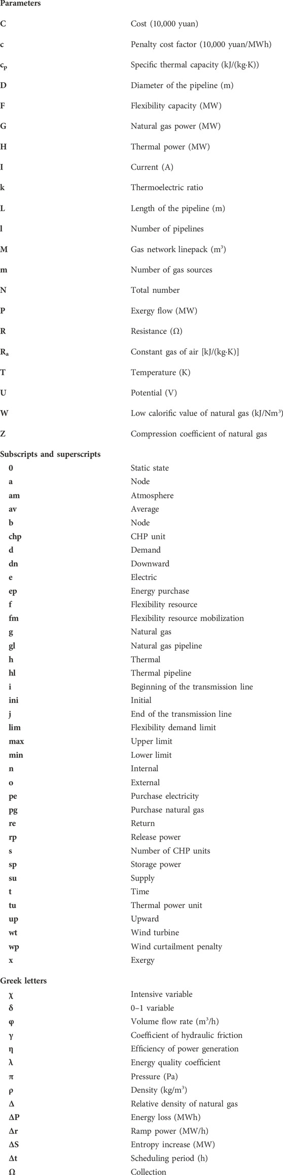
Nomenclature