Simultaneous series and shunt earth fault detection and classification using the Clarke transform for power transmission systems under different fault scenarios

1 Introduction

1.1 Background and motivation

The most challenging task in protecting transmission lines is detecting faults the power system faces at a reliable performance level. Transmission line faults based on nature in terms of resistance are divided into low-impedance faults (LIFs) and high-impedance faults (HIFs). The main distinction between them is that the increased impedance is within the path of the fault current, limiting the arc current. LIFs comprise single line-to-ground faults, phase-to-phase faults, etc. HIFs result from unwanted contact with power conductors that are poorly connected to surfaces, making it difficult to detect these faults using traditional protection relays (Ghaderi et al., 2017). Like the open conductor (OC), a pathway toward the ground is not always included in HIFs. The open conductor faults (OCFs), like the series HIFs, cause the circuit breaker to not open due to the direct opening bridle. This is followed by the descent of the conductor to the ground (Jeerings and Linders, 1991). In addition, the OC in the transmission lines (TLs) is a challenging problem in power system operation. As a result, the system’s stability suffers as the power transmitted over the line is lowered and healthy phases may be subjected to overloading. Furthermore, if the system is non-earthed, the voltage in the healthy phases may increase (Velez, 2014). Electric shocks and fire hazards generated by open conductor faults (OCFs) are also significant concerns regarding community safety, property failure, and losses. So, first and foremost, fast detection of OCFs is essential to transmission utilities (Abdel-Aziz et al., 2017). Because OCFs do not considerably increase current or voltage drop, distance protective relays, considered the TLs’ principal protection mechanism, cannot detect them. As a result, the distance relay does not trip, and the fault will continue to occur in the open connector until the connector falls to the ground and is detected by another protection relay. In some cases, an earth fault relay can identify this fault-based high value of current when the conductor falls on a surface with meager resistance; however, since it is considered a standby protective for TLs, it will suffer from a delay time.

1.2 Literature overview

According to the literature, there are two proposals for identifying OCFs in transmission systems. The negative sequence was the suggested technique for identifying open and down conductor faults, where the negative sequence to the positive sequence current portion is introduced (ALSTOM, 2017). Different artificial intelligence schemes, such as neural networks (Koley et al., 2014) and In (Shukla et al., 2017), utilized the wavelet and naïve Bayes classifier to detect the OCF in six-phase TLs. Most previous schemes, such as thresholds in ALSTOM (2017), do not fully define the OCF problem and offer specific practical implementation challenges. Furthermore, the robustness of the artificial neural network protection scheme proposed by Gilany et al. (2010) has several practical constraints to be fabricated, as the reliability of these systems is highly determined by the nature of the design and the level of changes made to it, such as higher increased loads. In Elmitwally and Ghanem (2021), detecting the fault, selecting the faulty phase, and identifying the fault point depended on measuring the three-phase current at the protective relay in superimposed components of compensated TLs. In Khoshbouy et al. (2022), the ratio for the phase voltage at the sending end to the sum of the ratio for the phase current for two ends in TLs, called pilot superimposed impedance, was used to detect interior and exterior faults competed to a predetermined value, which was estimated based on Thevenin impedance.

Furthermore, many algorithms have been introduced in the literature over the past 20 years to detect OCFs in electric distribution utilities. For instance, voltage unbalance over the feeder was measured to identify the OCFs using sensors (Vieira et al., 2019); however, these sensors need sophisticated communication between these devices. In addition, the proportion of the SC current was inspected in Jayamaha et al. (2017); this requires the installation of current sensors over the line to protect it and deal with numerous challenges that may be difficult to overcome. Other proposed approaches, such as that introduced in Silva et al. (2018), relied on installing a device that measures the second or third harmonics of the current and follows the changes that may occur due to faults. Other schemes of detecting OCFs relied on the data measured from phase-measuring units (Zanjani et al., 2012). However, this necessitated precise management between these units and the control center. The detection strategy presented in Adewole et al. (2020) to identify an open phase was based on the current imbalance prevalent during the occurrence of OCFs; however, it was only suitable for earthed distribution utilities. Additionally, the current arc value changes rapidly over time during HIFs, which presents another challenge for schemes that rely on measuring the variance in frequency components (FCs) of the current due to arcing. The concept behind this is extracting the transient change in the fault (Shukla et al., 2017). In addition, many research works have been published to identify the fault in TLs based on wavelet transform applications, such as discrete wavelet transform, wavelet packet transform, and single-wave entropy schemes. Numerous works used the discrete wavelet transform scheme because time–frequency localization can assess the transients during HIFs (Saravanababu et al., 2013). However, the schemes that rely on high-frequency components, as described in Ashok et al. (2019), result in weak discrimination between LIFs and HIFs. Conversely, algorithms such as those used in Rathore and Shaik (2015) relied on low-frequency components that failed to distinguish HIFs. It should be mentioned that incorporating between low and high frequencies was discussed using predetermined values in Shaik and Pulipaka (2015). However, the fault was not detected when switching a large load case because the value of the low-frequency component primarily relies on the value of the load current. Furthermore, research works (Usama et al., 2014) based on wavelet analysis focused on detecting earth faults, not OCFs. Accordingly, the difficulty in detecting and locating OCFs remarkably affects the state of OCFs on both sides of TL systems. In Asuhaimi Mohd Zin et al. (2015), fault detection and classification utilized discrete wavelet transform and back-propagation neural networks based on Clarke’s parallel-transmission transformation. The fault detection and classification of fault types that are triggered in three-phase TLs using the artificial neural network is described in Assadi et al. (2023). The proposed scheme can detect and classify several faults, including line-to-ground, line-to-line, double-line-to-ground, triple-line, and triple-line-to-ground faults. In Mahanty and Gupta (2007), the methodology for fault analysis uses current samples with the help of fuzzy logic. In this technique, only one end of the three-phase current samples was considered to achieve fault classification. The neural network was utilized for training, and a fuzzy view point was applied to gain an insight into the system and to reduce the complexity of the system (Dash et al., 2000). Jayabharata Reddy and Mohanta (2007) presents a real-time wavelet–Fuzzy combined scheme for digital relaying. The algorithm for fault classification utilizes wavelet multi-resolution analysis to overcome the complications combined with conventional voltage and current-based measurements due to the effect of fault inception angle, fault impedance, and fault distance. No scheme has proven its superiority and effectiveness in all fault scenarios. Thus, new effective solutions are therefore needed.

1.3 Contributions and novelty

This work discusses a detection scheme that relies on the Clarke transform conversion for the current signals in TLs, such as the OCF on both sides and the OCF on a single side, followed by an earthed fault on another side through LIFs and HIFs. The sign of all current Clarke components is the primary key for distinguishing between all types of simultaneous LIFs and HIFs. The alternative transient program (ATP) package simulates a 500 kV–150-mile transmission line. The behavior of the proposed schemes is tested and validated considering different fault scenarios with different fault locations, inception angles, fault resistance, and noise.

Furthermore, the proposed schemes are extended to another transmission line, such as the 400 kV–144 km line. The obtained results demonstrated the effectiveness and reliability of the proposed scheme in detecting simultaneous faults, LIFs, and HIFs correctly in 20 mS.

The novelty in the proposed scheme and the essential features that verify the accomplishment achievement of its purpose effectively compared to the preceding approaches are as follows:

• Functionality: It can correctly discriminate between OCFs (series faults), two types of broken conductors together with earth faults (shunt fault) occurring after a short period (simultaneous earth faults), HIFs, and LIFs. These faults are correctly detected at both ends compared to other existing schemes that see these faults at a single end.

• Cost: It does not require the installation of new current transformers because it relies on the measurements at both ends and does not use the high sampling frequency compared to other existing schemes.

• Flexibility and independency: It utilizes powerful threshold values at both ends and relies on a detailed description study in this manuscript. Consequently, the proposed threshold values are appropriate for all fault scenarios and do not need adaptive values under variations of network configuration (independent of the system topology) or variations in load current.

• Speed: It has advantages in terms of speed and visibility in its application compared with other existing schemes because it corrects discrimination using communication links between both ends already installed.

1.4 Organization

The rest of the manuscript is organized as follows: Section 2 clarifies the fundamental problem investigated in this work. The proposed fault detection strategy is introduced in Section 3. In Section 4, the behavior assessment for the proposed scheme is conducted using ATP to examine the ability to identify the fault. In Section 5, a comparison is made between the proposed scheme and other schemes presented in the literature. Finally, Section 6 is dedicated to the conclusion drawn and future work directions. A schematic overview of the proposed scheme’s assessment steps and the work’s organization is given in Figure 1.

FIGURE 1

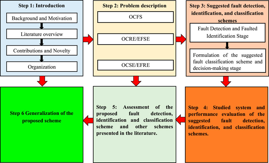
FIGURE 1. Schematic overview of the proposed scheme’s assessment steps and work organization.

2 Problem description

Figure 2 shows both types of OCFs (series faults) and broken conductors together with earth faults (shunt faults) occurring after a short period (simultaneous earth faults). Figure 2A illustrates an OC from two sides. The OCF can occur if the bridle wire is open and banned at two sides, as seen in Figure 2B. An OC (broken conductor) happens on one end, followed by a down conductor appearing on the opposite end (simultaneous faults). As a result of opening the same conductor, the down conductor takes time to touch the soil, depending on the height of the conductor above the ground and the acceleration due to gravity. The surface/soil resistance value significantly affects the fault current’s value. The OC in the receiving end side at 0.08 s is followed by a shunt fault across LIFs and HIFs at the sending end side, as illustrated in Figure 2C. The OC at the sending end side, after 0.08 s, is followed by a shunt fault across LIFs and HIFs at the receiving end side, as illustrated in Figure 2D. Consequently, HIFs can be termed as shunt faults disregarding the OC case (Banner and Don Russell, 1997). HIFs usually occur beside the OC near the receiving end and touch a surface of the ground or by other elements at the sending end side of the transmission system.

FIGURE 2

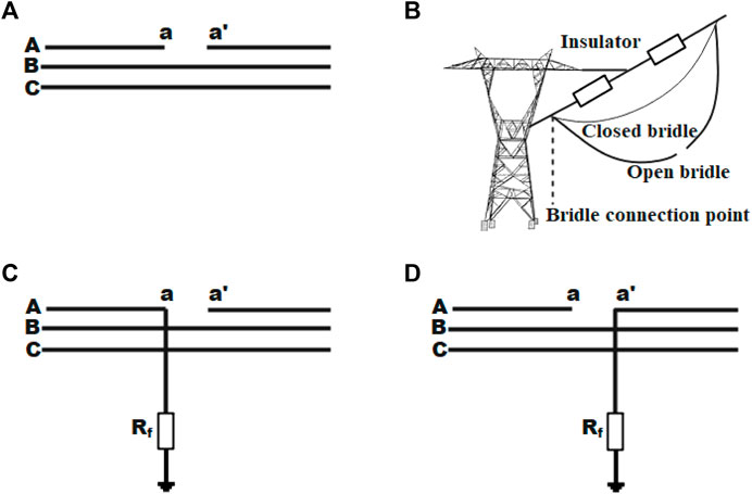
FIGURE 2. Presentation of an open conductor and simultaneous faults for phase A: (A) open circuit fault; (B) exhibition of OCF; (C) OC at the receiving end followed by a shunt fault at the sending end (denoted OCRE/EFSE); (D) OC at the sending end followed by a shunt fault at the receiving end (denoted OCSE/EFRE).

HIFs are affected by several factors, including the material of the ground surface, moisture of the surface, levels of voltage, and weather circumstances. One factor that significantly impacts the characteristics of HIFs is surface humidity, where surfaces with high humidity lead to increased fault current magnitude (Kavaskar and Kant, 2019). In addition, HIFs occurring through different materials could lead to other voltage–current characteristics. Materials that touch down-conductors from the tower may include tree branches, lawns, gravel, deep gravel, thin gravel, asphalt, concrete, sand, crushed stone, board blocks, and cement. Recently, the down conductor problem in distribution networks has been solved, as explored by Esmail et al. (2022). This motivated the authors to investigate solving the same problem in transmission line systems.

This work investigates the problem of detecting simultaneous series and shunt earth faults in conventional protection relays in the TL by applying different simulation cases in power systems. All simulated cases were taken at 130 miles from the sending end, which emphasized the actual performance of the protection relay, which is not seen in these types of faults owing to the small fault current value. At the same location, various faults were implemented, with OCFs and an OC at the receiving end side, followed by an earth fault on the sending end side, and an OC at the sending end side, followed by an earth fault on the receiving end side.

The traditional protection performance under these simulated faults was examined, as shown in Figure 3, by computing the discrete Fourier transform (DFT)-based amplitude for three-phase currents and imbalance ratios (I₂/I₁, I₀/I₁), considering OCFs at both ends. Conventional protection cannot detect the broken conductor fault by investigating the results. The value for the current amplitude of phase A and I₂/I₁, I₀/I₁ ratios at the sending end provide a maloperation for the device. Furthermore, the current amplitude of phase A gives (10–15) % of its values at normal operation.

FIGURE 3

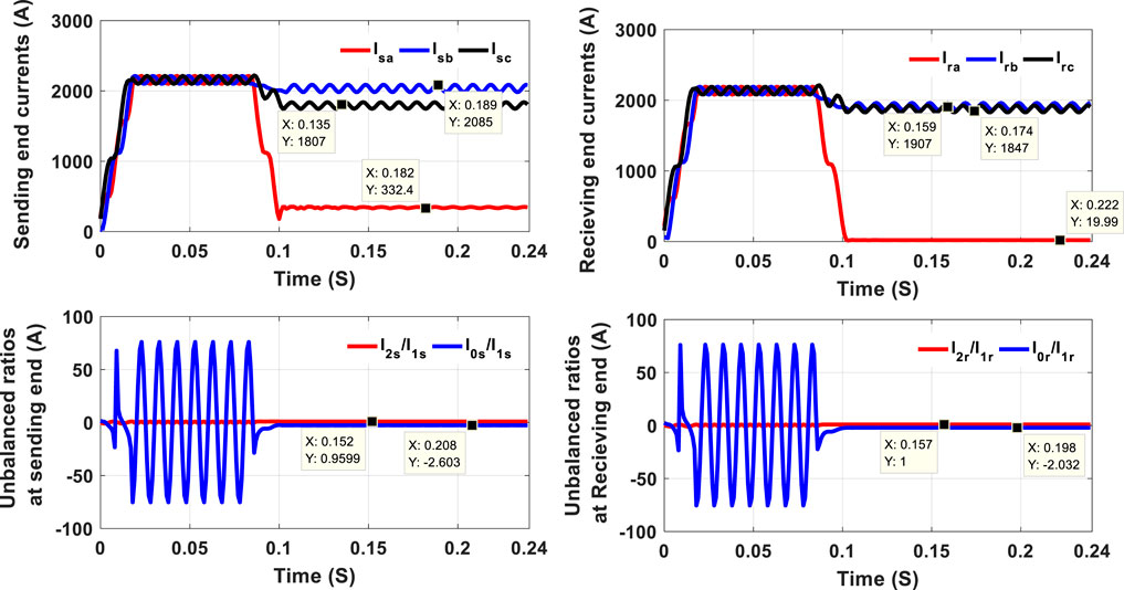
FIGURE 3. DFT-based amplitudes for three-phase currents and imbalance ratios considering OCFs at both ends.

In addition, the behavior of the traditional protective relay under these simulated faults was examined, as shown in Figure 4, by computing the DFT-based amplitude for three-phase currents and ratios (I₂/I₁, I₀/I₁) at both ends. The value of the current amplitude of phase A gives (140–160) % from its value at normal operation at the sending end, which is considered a shunt fault, but the value of the same phase A gives (10–15) % from its values at normal operation at the receiving end, which is considered a series fault. Moreover, the values of both ratios (I₂/I₁, I₀/I₁) at both ends resulted in a malfunction for both protection devices. Figure 5 shows the DFT-based amplitudes for three-phase currents and unbalanced ratios under an OC at the protective relay aspect, followed by earth fault in the reverse protection relay aspect at both ends. The recorded amplitude for phase A at the sending end gives (10–15) % of its values at normal operation, demonstrating that its devices cannot detect this fault condition. However, at the receiving end, the recorded amplitude for the same phase gives (140–160) % of its value at normal operation, which is considered a shunt fault. Furthermore, the unbalanced ratios at both ends cannot provide any detection for this type of fault condition. These results highlighted the incapability of traditional protection strategies in detecting these types of faults.

FIGURE 4

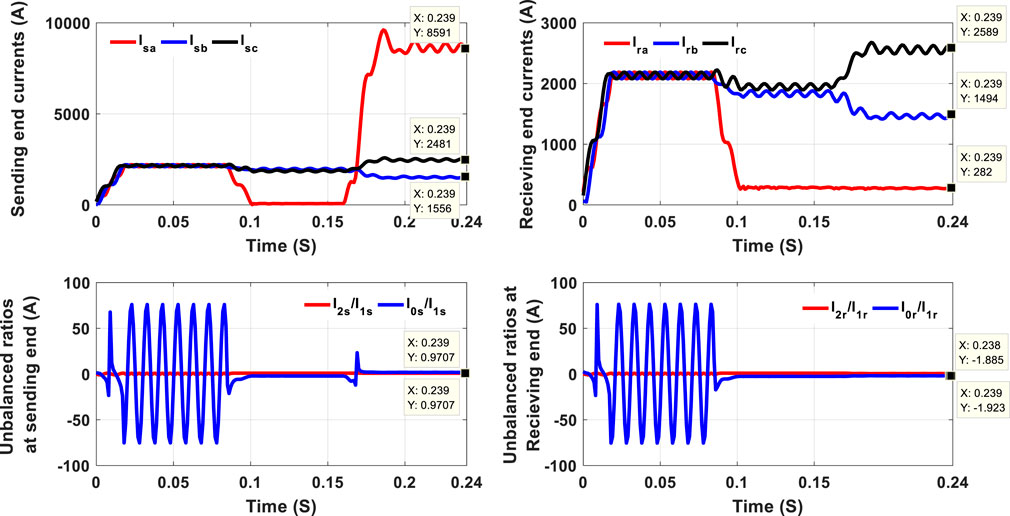
FIGURE 4. DFT-based amplitudes for three-phase currents and unbalanced ratios considering OCFs at the receiving end followed by earth fault at the sending end (OCRE/EFSE) at both ends.

FIGURE 5

FIGURE 5. DFT-based amplitudes for three-phase current and unbalanced ratios considering OC at the sending end followed by earth fault at the receiving end (OCSE/EFRE) at both ends.

3 Suggested fault detection, fault identification, and classification schemes

3.1 Fault detection, identification, and classification

The proposed schemes comprise different stages: fault detection, identification, and classification, as declared in Figure 6. As illustrated in Figure 6, the introduced scheme relies on the existing phasor measurement unit at the high-voltage side. Each phasor measurement monitors the three-phase currents’ magnitudes. Phasors are considered the primary tool for analyzing the power system in its steady state or transient situations, so phasor estimation is quite essential for protection applications. Estimating the voltage and current phasor is performed concerning one frequency, which is usually the fundamental power frequency. A phasor measurement unit, or synchrophasor, is a device that measures a power system’s synchronized current phasor. Synchronization among phasor measurement units is achieved by same-time sampling of voltage and current waveforms using a famous synchronizing signal. The ability to calculate synchronized phasors makes the phasor measurement unit one of the most important measuring devices in the future of power system monitoring and control. Precise synchronization of sampling clocks throughout the power system became possible with the advent of the global positioning system (GPS) satellite system. Although the precision of synchronization was not very good in the early years of the system, at present, it is possible to achieve synchronization accuracies of 1 µs or better.

FIGURE 6

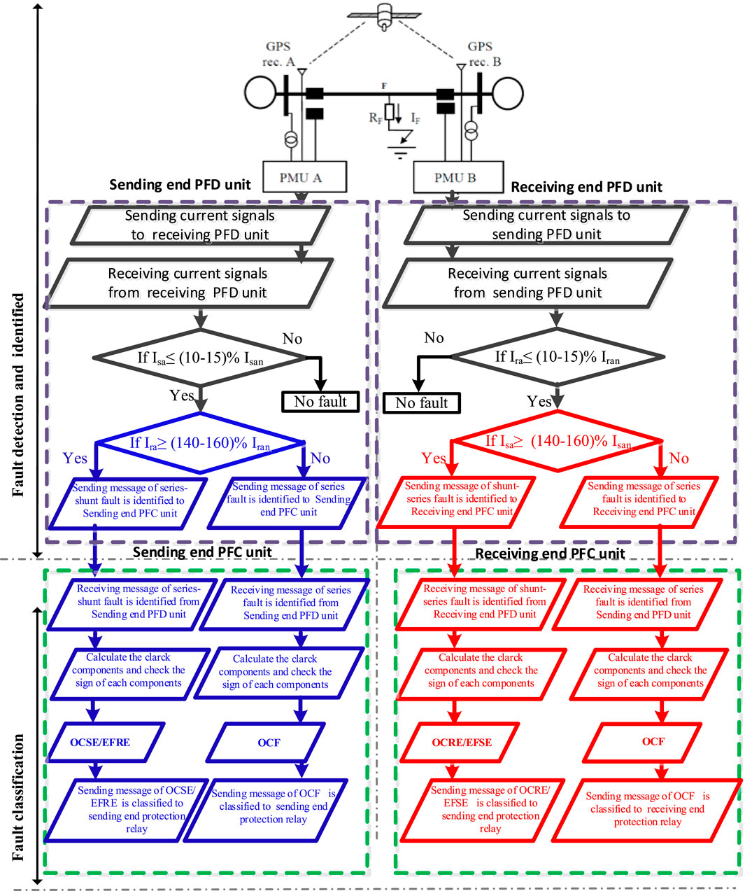
FIGURE 6. Flow chart of the proposed fault detection, identification, and fault classification schemes.

The applicability and feasibility of the proposed schemes are clear. Nevertheless, the proposed scheme needs communication links between both ends (sending and receiving end) to detect, identify, and classify the fault. This communication link between both ends is used to send and receive three-phase currents’ magnitudes for sending and receiving ends in the proposed fault detection (PFD) unit at both ends. The presented scheme is embedded in the PFD unit on both ends to detect and identify these faults when one or two conditions are verified. In the sending end PFD unit, the first condition is proving if the obtained sending end current for phase a at fault is equal to or less than (10–15) % of the sending end current for phase A at normal operation. The second condition is verifying if the obtained receiving end current for phase A at fault is equal to or more than (140–160) % of the receiving end current for phase A at normal operation. Furthermore, in the receiving end PFD unit, the first condition is verifying if the obtained receiving end current for phase A at fault is equal to or less than (10–15) % of the receiving end current for phase A at normal operation. The second condition is verifying if the obtained sending end current for phase A at fault is equal to or more than (140–160) % of the sending end current for phase A at normal operation. The security attribute for the presented algorithm is achieved under unbalanced load conditions. Thus, the obtained sending end or receiving end current for phase A at fault is more than (140–160) % of the sending end or receiving end for phase A at normal operation. According to the proposed detection scheme, this is the second condition monitoring if the first condition is verified.

Consequently, the proposed scheme is not affected by unbalanced load conditions. On the other hand, the presented algorithm is susceptible to consideration because the computed current signal significantly increases to specific high ratios according to the fault type. The threshold values ((10–15) % and (140–160) %) are selected based on the detail analysis under all possible fault conditions in Section 2. The expected threshold values under these faults are as follows:

3.1.1 Series fault

Under series faults, the obtained sending end current for phase a at fault is equal to (10–15) % of the sending end current for phase a at normal operation in the sending end PFD unit, and the obtained receiving end current for phase a at fault is less than (10–15) % of the receiving end current for phase a at normal operation in the receiving end PFD unit, which means that only the first condition is verified, and then sending a message of series fault being identified to the sending end PFC unit. Accordingly, the process of the fault classification PFC unit starts after receiving a message that the series fault is identified from the sending end PFD unit.

3.1.2 Series–shunt fault

Under the series–shunt fault, in the receiving end PFD unit, similarly, the first condition is verified. The second condition is checked (if the obtained sending end current for phase a at fault is equal to or more than (140–160) % of the sending end current for phase a at normal operation) and verified. If two conditions are verified, the PFD unit sending a message of series–shunt fault is identified to the sending end PFC unit, and the flow of fault classification starts after receiving this message in its unit.

3.1.3 Shunt–series fault

Under shunt–series fault, the first condition is verified in the sending end PFD unit. The second condition is detected (if the obtained receiving end current for phase a at fault is equal to or more than (140–160) % of the receiving end current for phase a at normal operation) and verified. If two conditions are verified, and then receiving a message of shunt–series fault is identified from the receiving end PFD unit, the flow of fault classification starts in the receiving end PFC unit.

According to the previous subsection, fault detection, identification, and fault classification are performed in both PFD units at both ends. Furthermore, the first step of fault classification is checked in both PFC units using PFC units on both ends, as seen in Figure 6. The fault classification procedure further takes place after calculating the Clarke components and checking the sign of each component using the chart seen in Figure 7. Then, all PFC units in both sending and receiving ends send the message of fault classification to the sending and receiving end protection relay, respectively.

FIGURE 7

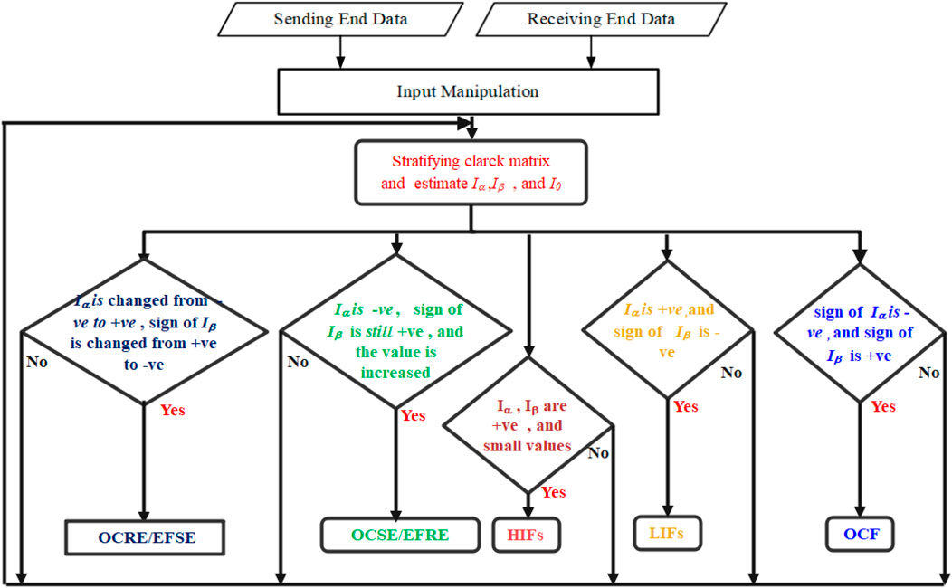
FIGURE 7. Flow chart of the proposed fault classification scheme in PFC units at both ends.

3.2 Formulation of the suggested fault classification scheme and decision-making stage

In the PFC units, the formula of the suggested fault classification is examined under some critical insights into un-transposed and transposed TLs. In this regard, the impedance matrix is symmetrical in the un-transposed case (symmetrical space between the conductors). In a symmetrical space between the conductors, the self or diagonal terms are generally unequal, and neither is the mutual or off-diagonal term in the impedance matrix. The current flowing in any one conductor will induce voltage drops in the other two conductors, which may be unequal even if the currents are balanced. Asymmetric voltage drops caused by the mutual impedances are unequal. This issue can be solved by making the TLs a perfectly transposed line in which the three sections have equal lengths. The perfect transposition results in the same total voltage drop for each phase conductor and equal average series self-impedance of each phase conductor. This effect applies to the average series phase mutual impedance and the average shunt phase mutual susceptance. Consequently, the phase impedance for a perfectly transposed single circuit is symmetric. Applying an entire transpose scheme suffers from expensive costs and inconvenience. Accordingly, the line may be transposed at one or two locations along the line route. This configuration provides a symmetrical impedance matrix.

In the proposed fault classification procedure, the output of the Clarke matrix is reflected in signals of the phase currents to detect various OCFs in un-transposed and transposed TLs precisely. The time-domain transformation is used with Clarke components, denoted as α, β, and 0, which are extracted as follows:

$\left[\begin{array}{c}{I}_{\alpha }\\ I_{\beta }\\ I_0\end{array}\right]=\left[\begin{array}{ccc}2/3& -1/3& -1/3\\ 0& 1/\sqrt{3}& -1/\sqrt{3}\\ 1/3& 1/3& 1/3\end{array}\right]\left[\begin{array}{c}{I}_a\\ I_b\\ I_C\end{array}\right].(1)$

The Clarke components are represented by Eq. 1, considering phase a as a reference, and two other Clarke components concerning phases b and c. In general, the same zero “0” component exists for any reference, whereas phases a, b, and c have three “β” components. These components are called aerial modes 1, 2, and 3 when OCFs or simultaneous earth faults occur. First, when conductor a opens, as shown in Figure 2B, one can note the following for Clarke’s components:

$I_{\alpha }=\frac{2}{3}{I}_a-\frac{1}{3}{I}_b-\frac{1}{3}{I}_c,(2)$

$I_{\beta }=\frac{1}{\sqrt{3}}\left(I_b-I_c\right),(3)$

$I_0=\frac{1}{3}\left(I_a+I_b+I_c\right).(4)$

Second, when the simultaneous earth fault at phase a happens, as shown in Figure 2C or Figure 2D, one can find that Clarke’s matrix components change as follows:

$I_{\alpha }=\frac{2}{3}{I}_a-\frac{1}{3}{I}_b-\frac{1}{3}{I}_c,(5)$

$I_{\beta }=\frac{1}{\sqrt{3}}\left(I_b-I_c\right),(6)$

$I_0=\frac{1}{3}\left(I_a+I_b+I_c\right).(7)$

Evaluating the three components of the Clarke matrix shows that aerial modes 1 and 2 best identify OCFs and simultaneous earth faults. The values of aerial modes 1 and 2 are 0 under healthy conditions. If OCFs occur, analysis of Clarke’s matrix components reveals that the value of aerial mode 1 is negative and the value of aerial mode 2 is positive, as shown in Figure 7.

The same components are examined when LIFs are involved in the investigation. Aerial mode 1 is found to have a positive sign, while aerial mode 2 has a negative sign. This means that OCFs and LIFs are entirely different when compared to each other. Moreover, the sign of aerial modes 1 and 2 is positive, and their values are low if HIFs occur. In addition, if an OCRE/EFSE fault occurs, it will be found that the sign of aerial mode 1 changes from negative to positive, and the sign of aerial mode 2 changes from positive to negative. Furthermore, the sign of aerial mode 1 is negative, and its value increases, while the sign of aerial mode 2 is positive, and its value increases when an OCSE/EFRE fault occurs.

4 Studied system and performance evaluation of the suggested fault detection, identification, and fault classification schemes

Figure 8A shows the single-line diagram of the 500 kV, 138-mile TL simulated in the ATP/EMTP program. The ATPDraw software is an interface to implement the system (Prikler and Høidalen, 2009). This TL model is a benchmark in ATPDraw software, and it is represented using the three-phase JMARTI frequency dependence model in the ATPDraw field using the line/cable module (Prikler and Høidalen, 2009). The JMARTI representation is a frequency-fitted model in a specific frequency range. The JMARTI model is utilized to apply the simulated line and therefore take waveforms for the fault case in evaluating the proposed schemes. The results taken in this study are the same as the results taken on the same system in Elkalashy, 2014; Elkalashy et al., 2016. For simultaneous series and shunt earth fault detection and classification using the Clarke transform for TLs under different fault scenarios, the line parameters have been extracted, and results show that the self-impedance of this line, for a length of 138 miles, is 0.1431 + j1.2999 Ω, while that of the mutually linked one is 0.1052 + j 0.6249 Ω, according to the retrieved line parameters. Using a mutually linked RL circuit, Thevenin’s equivalent impedance at buses S and R is expressed as R₁ = 1.0185 Ω, L₁ = 50.929 mH and zero sequences are R₀ = 2.037 Ω, L₀ = 101.85 mH at bus S and R₁ = 1.0185 Ω, L₁ = 42.85 mH, R₀ = 1.735 Ω, L₀ = 101.85 mH at bus R. The TL configuration is illustrated in Figure 8B, where the DC resistance is 0.05215 Ω/mile, the outer diameter of the conductor is 1.602 inch, and the inner radius of the tube is 0.2178 inch. The sky wires are solid; their dc resistance is 2.61 Ω/mile, and the outer diameter is 0.386 inch. The resistivity of the soil is equal to 100 Ω.

FIGURE 8

FIGURE 8. Single-line diagram (SLD) of the simulated TL system and the selected tower: (A) SLD; (B) tower configuration.

The JMARTI model is fundamentally depicted by the rational approximation of the characteristic impedance (Zc) and by the elements of the propagation matrix (H). The JMARTI model’s fitting technique is based on the theory of asymptotic approximations of magnitude functions. This rational approximation technique starts with only real poles and zeros and, therefore, real state variables. A small error in simulation for 500 kV TL is found using system verification in the ATPDraw software program. In Bañuelos-Cabral et al. (2019), the model’s accuracy was increased by using only real poles through vector fitting.

The simulation studies are carried out to assess the suggested fault detection, identification, and fault classification scheme performance under various OCFs and simultaneous earth faults (OCSE/EFRE, OCSE/EFRE) in un-transposed and transposed TLs while sampling the current signal at 200 kHz, such that a conductor opens on both sides (OCFs): an OC on the relay aspect at 0.08 s, followed by a shunt fault on the opposite aspect due to low resistance of 3 Ω (OCSE/EFRE), and an OC on the relay’s opposite aspect at 0.08 s, followed by a shunt fault caused by 3 Ω low resistance (OCRE/EFSE). The two kinds are repeated with HIFs and LIFs.

Furthermore, the proposed fault detection, identification, and fault classification schemes were verified during the recorded signals considering noise impacts as in practical TLs. Therefore, the recorded error signals captured in the proposed schemes are contaminated with white Gaussian noise, with a 30–60 dB signal-to-noise ratio. The proposed schemes are unaffected by any signal-to-noise ratio; however, a signal-to-noise ratio equal to 40 dB is used in this work.

First, we suppose an OCF occurs at 130 miles from the sending end. In that case, the values of Clarke components are shown in Figure 9 considering four scenarios (transposed line without noise effect, transposed line with noise effect, un-transposed line without noise effect, and un-transposed line with noise effect. When the conductor opens, one can find that phase a’s current value decreases to the lowest value compared to its value before opening the conductor. For phase current b, a decrease in the current value up to 1,983 A occurs. Then, an increase in the current value up to 2,040 A occurs, followed by a reduction in its value up to 1,887 A and then an increase in its value up to 1965 A. For phase current c, an increase in the current value up to 2,193 occurs, followed by its decrease to 1995 A, then increases to 2,044 A, followed by a reduction in its value to 1873 A, taking into account that the value of phase current b is higher than that of phase current c, after steadying their values after a series of fluctuations. This, in turn, resulted in the sign of aerial modes 1 and 2 being negative and the sign of the grounding mode being positive. Based on the successive change in the values of phase currents b and c, it is possible to determine when the opening occurs (0.08 s) as the instant before the change.

FIGURE 9

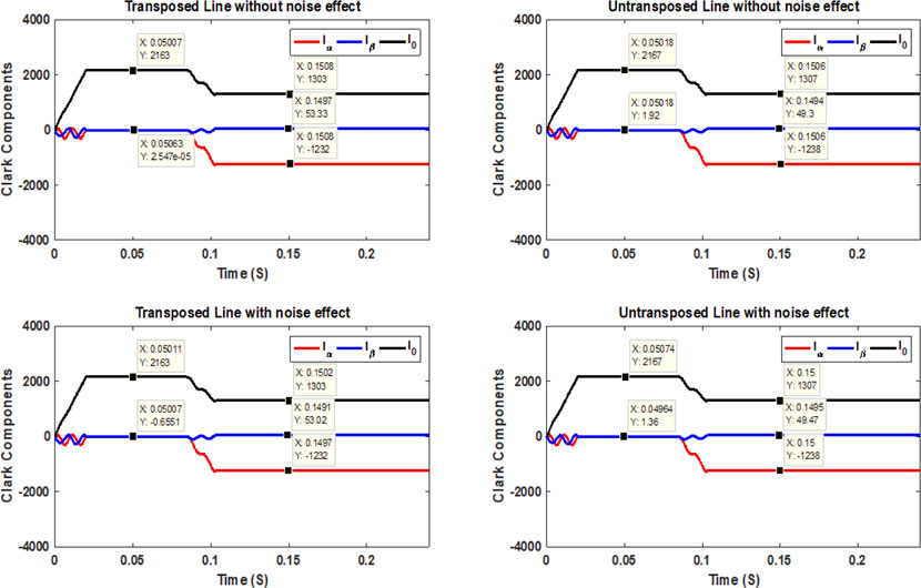
FIGURE 9. Clarke comments on the sending end currents at OCFs.

Second, the values of the Clarke components in Figure 10 are shown when the OCSE/EFRE occurs at 130 miles from the sending end. In this figure, aerial mode 1 has a negative sign at the opening instant of the conductor (0.08 s), and its sign is still negative at the instant of a down conductor (0.16 s). When phase a touches the ground, one can notice that the current value of phase a remains at its minimum value, which reaches 331.3 A after opening the same phase a. In addition to the high value of phase current b (2667 A), compared to its exact value after opening phase a, as in the OCF case, phase c also causes a decrease in its current value to 1,310 A compared to its exact value after opening phase a. The high value of phase current b makes aerial mode 2 have a positive sign at the open conductor instant (0.08 s). Its value increases at the down conductor instant (0.16 s). The grounding mode has a positive sign, and its value slightly increases at the down conductor instant. Furthermore, based on the change in the values of phase currents b and c, it is possible to determine when the conductor was down (i.e., before this change). Third, the values of the Clarke components for OCRE/EFSE occurring at 130 miles from the sending end are shown in Figure 11 based on the values of the three-phase currents. As seen in this figure, the sign change from negative to positive for aerial mode 1 is caused by increasing the value of phase current a at the contact with the ground instant, which reaches 3,678 A, decreasing the value of phase current b (reaches 1,226 A) and increasing the value of phase current c, which reaches 2,844 A. Furthermore, aerial mode 2 has a positive sign at the open conductor instant (0.08 s) and changes to a negative sign at the down conductor instant (0.16 s). In comparison, the grounding mode has a positive sign, instantly increasing its value at the down conductor. On the other hand, the LIF was examined as a simulated case to state that the case is considered simple from the point of view of protection systems, giving a high fault current value.

FIGURE 10

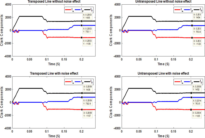
FIGURE 10. Clarke comments on the sending end currents at OCSE/EFRE.

FIGURE 11

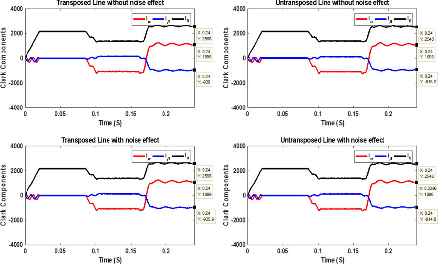
FIGURE 11. Clarke comments on the sending end currents at an OCRE/EFSE.

Fourth, the values of the Clarke components are shown in Figure 12 for a condition of LIF happening at 130 miles away from the sending end. Aerial mode 1 has a positive sign at the LIF instant, and aerial mode 2 has a negative sign at the same instant. The grounding mode, however, has a positive sign, and its value increases at the LIF instant. The signs of Clarke components are caused by increasing the phase current reaches 3,703 A for phase a, 2,021 A for phase b, and 2,325 A for phase c after the LIF instant.

FIGURE 12

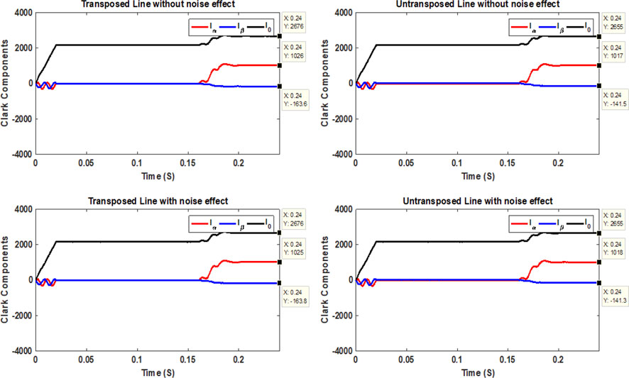
FIGURE 12. Clarke comments on sending end currents at the LIF.

Fifth, for a HIF occurring at 130 miles away from the sending end, the Clarke components values are given in Figure 13.

FIGURE 13

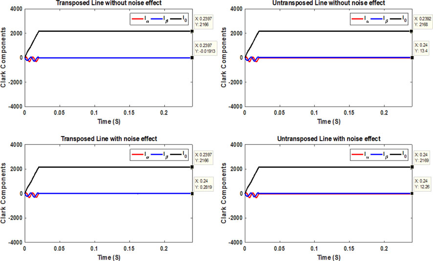
FIGURE 13. Clarke comments on sending end currents at the HIF.

In most cases, aerial modes 1 and 2 have a positive sign at the HIF. The value of the grounding mode increases at the moment of a HIF and has a positive sign at 0.16 s. These signs are caused by increasing the three-phase currents after the HIF instant (reaches 2,166 A).

5 Assessment of the proposed fault detection, identification, and fault classification schemes and other schemes presented in the literature

The suggested fault detection, identification, and fault classification scheme’s behavior was verified distinctly by comparing it with the discrete wavelet transform (DWT)-based algorithm (Abd-Elhamed Rashad et al., 2020) through simulation results. First approximation A₁ and first detail D₁ coefficients are extracted from three-phase current signals and are examined to detect various OCFs and simultaneous earth faults.

The following are the stages followed for the detection and classification of faults:

For the three-phase current signals (i_a, i_b, and i_c), apply single-level decomposition using db1 to obtain high-frequency components (D₁: 50–100 kHz) and low-frequency components (A₁: 0–50 kHz). Parameters are estimated at this stage using Eq. 8 expressions.

$\begin{array}{c}{M}_a\left(k\right)=\mathit{max}\left|{\left.i_{a\left(n\right)}\right|}_{n-k-N+1^k}\right.,\\ M_b\left(k\right)=\mathit{max}\left|{\left.i_{b\left(n\right)}\right|}_{n-k-N+1^k}\right.,\\ M_c\left(k\right)=\mathit{max}\left|{\left.i_{c\left(n\right)}\right|}_{n-k-N+1^k}\right..\end{array}(8)$

Here, n represents a sample demand in a sliding window covering a complete cycle, and N is the total number of samples in a process. Furthermore, one should calculate the highest absolute values of A₁ for the three-phase current signals (M_a, M_b, and M_c) at sample k.

Using the mathematical formulas in Eq. 9, determine the absolute decomposed currents’ detail coefficients (S_a, S_b, and S_c) as follows:

$\begin{array}{c}{S}_a\left(k\right)={\displaystyle \sum _{n=k-N+1}^k}\left|\left.{D1i}_{a\left(n\right)}\right|\right.,\\ S_b\left(k\right)={\displaystyle \sum _{n=k-N+1}^k}\left|\left.{D1i}_{b\left(n\right)}\right|\right.,\\ S_c\left(k\right)={\displaystyle \sum _{n=k-N+1}^k}\left|\left.{D1i}_{c\left(n\right)}\right|\right..\end{array}(9)$

Then, determine the differences in the absolute sum value for the three-phase current signals (H_a, H_b, and H_C) as follows:

$\begin{array}{c}{H}_a=\left|\left.S_a-S_b\right|\right.,\\ H_b=\left|\left.S_b-S_c\right|\right.,\\ H_c=\left|\left.S_c-S_a\right|\right..\end{array}(10)$

Next, determine the approximation coefficient ratios (R_a, R_b, and R_c) to detect OCFs.

$\begin{array}{c}{R}_a=\left|\left.M_a/M_b\right|\right.,\\ R_b=\left|\left.M_b/M_c\right|\right.,\\ R_c=\left|\left.M_c/M_a\right|\right..\end{array}(11)$

Finally, if the following criteria are met, the OCF is declared confirmed.

None of the M values exceed the predetermined M_th value, as expressed in Eq. 12.

$M_a<M_{th}and{M}_b<M_{th}and{M}_c<M_{th}.(12)$

One of the H values is higher than the threshold value H_th and remains there for more than 20 ms, as expressed in Eq. 13.

$H_a>H_{th}or{H}_b>H_{th}or{H}_c>H_{th}.(13)$

One or more of the R ratios exceeds 1.

$R_a>1or{R}_b>1or{R}_c>1.(14)$

It must be emphasized that the predetermined values in this platform (M_th and H_th) are determined based on the pre-fault (M_a, M_b, and M_c) with no operator interference (Abd-Elhamed Rashad et al., 2020).

5.1 Cases studied

Distinctive fault types across the TL length were evaluated through various fault situations (locations, inception angles, and fault resistance values) to explain the efficacy of the suggested schemes in detecting simultaneous OCSE/EFRE and OCSE/EFRE. The cases can be organized as follows to detect and classify faults successively:

Case 1:. OCFs at different locations and fault time occurrence (inception angle ϕ in degrees).

Case 2:. OCRE/EFSE at different locations and fault time occurrence considering fault resistance effects.

Case 3:. OCSE/EFRE at different locations and fault time occurrence considering fault resistance effects.

Case 4:. LIF and HIF at a specific location and specific fault time occurrence considering fault resistance effects.

5.2 Response of fault detection, identification, and fault classification schemes

5.2.1 Simulation results: case 1

Two test scenarios in case 1 are studied to determine the proposed scheme’s ability to detect and classify faults correctly. First, we suppose an OCF occurring 13.8 miles from the sending end at a fault inception angle set to 0°. In this case, the values of Clarke components are presented in Table 1 for the transposed TL without the noise effect in the first row, the transposed line with noise effect in the first shadow row, the un-transposed line without noise effect in the third row, and the un-transposed line with noise effect in the second shadow row.

TABLE 1

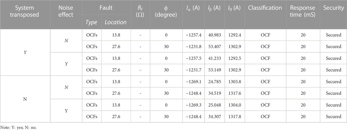
TABLE 1. Results of OCF fault detection, identification, and fault classification using the proposed schemes for the considered transposed and un-transposed lines with and without noise effect.

As shown in all previous tables, changing the fault location and ϕ has no effect on the results of the proposed scheme. Moreover, the suggested fault detection, identification, and classification schemes have identified all of them correctly.

The results of the DWT-based algorithm (Abd-Elhamed Rashad et al., 2020) in the same cases are also where the values of (M_a, M_b, and M_c), (H_a, H_b, and H_c), and (R_a, R_b, and R_c) are calculated in the four scenarios considered (the transposed line without noise in Table 2 in the first row, the transposed line with noise effect in the first shadow row, the un-transposed line without noise effect in the third row, and the un-transposed line with noise effect in the second shadow row.

TABLE 2

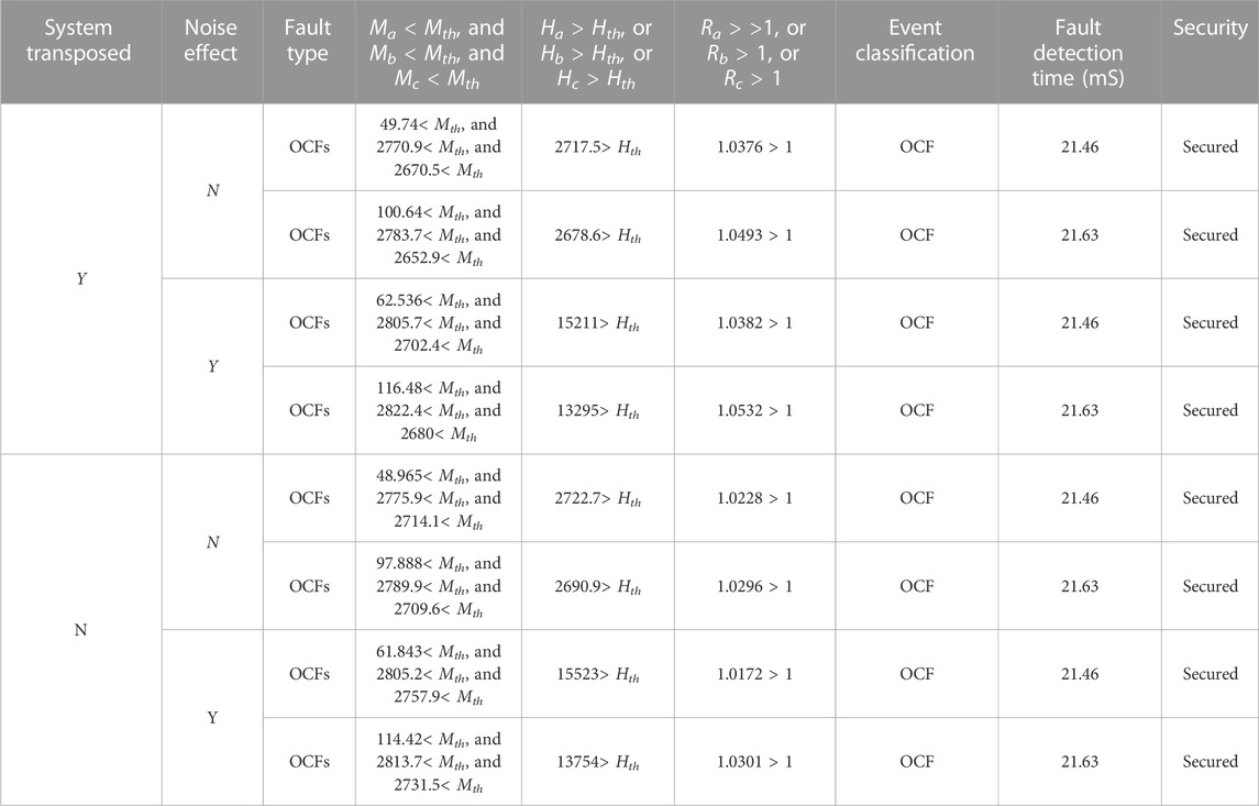
TABLE 2. Results of OCF fault detection, identification, and fault classification using the DWT-based algorithm for the considered transposed and un-transposed lines with and without noise effect.

As shown in the previous results, fault detection time in the DWT-based algorithm is greater than that in the suggested proposed schemes.

5.2.2 Simulation results: case 2

The security of the proposed schemes was verified by changing the fault resistance values and fault locations; different fault inception angles were examined with OCRE/EFSE. In this case, the values of the Clarke components are presented in Table 3 for the transposed line with no noise in the first row, the transposed line with noise effect in the first shadow row, the un-transposed line without noise effect in the third row, and the un-transposed line with noise effect in the second shadow row.

TABLE 3

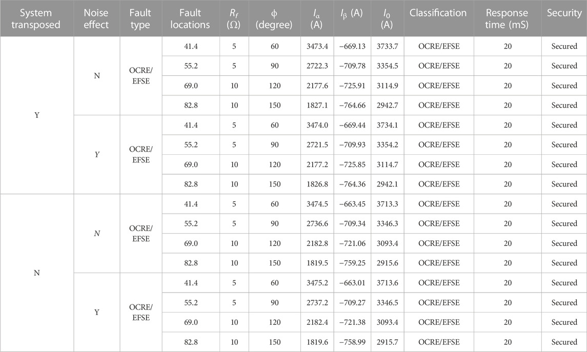
TABLE 3. Results of OCRE/EFSE fault detection, identification, and fault classification using proposed schemes for the considered transposed and un-transposed lines with and without noise effect.

This table shows that changing fault locations, fault resistances, and fault inception angles does not affect the effectiveness of the proposed fault detection, identification, and fault classification scheme.

Similarly, the results of the DWT-based algorithm (Abd-Elhamed Rashad et al., 2020) in the same cases are presented. The values of (M_a, M_b, and M_c), (H_a, H_b, and H_c), and (R_a, R_b, and R_c) are calculated considering the four scenarios, as shown in Table 4, respectively. As shown in this table, M_a > M_th and M_c > M_th are unsatisfied, which was caused by small fault resistance values. In such cases, the DWT-based algorithm failed to detect this type of fault and can be considered insecure against small values of fault resistances.

TABLE 4

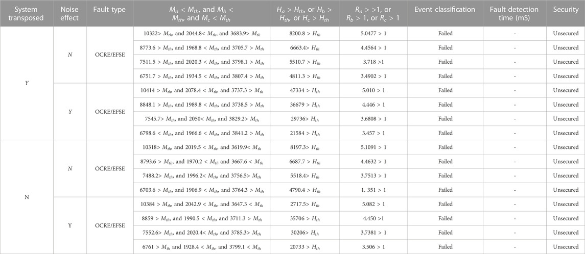
TABLE 4. Results of OCRE/EFSE fault detection, identification, and fault classification using the DWT-based algorithm for the considered transposed and un-transposed lines with and without noise effect.

5.2.3 Simulation results: case 3

The proposed fault detection, identification, and fault classification schemes were examined considering OCSE/EFRE at different locations, inception angles, and fault resistance values. In this case, the values of Clarke components are shown in Tables 5 for the investigated scenarios, respectively. This table shows that changing fault locations, fault resistances, and fault inception angles does not affect the proposed fault detection, identification, and classification schemes.

TABLE 5

TABLE 5. Results of OCSE/EFRE fault detection, identification, and fault classification using the proposed schemes for the considered transposed and un-transposed lines with and without noise effect.

Furthermore, as seen in Table 5, the signs of aerial modes 1 and 2 and ground mode are–ve, +ve, and +ve, respectively, at different fault locations, inception angle, and fault resistance values. Furthermore, the configuration of TL and noise impact does not affect the proposed fault detection, identification, and fault classification schemes. The DWT-based algorithm (Abd-Elhamed Rashad et al., 2020) was also examined as in the previous cases. The values of (M_a, M_b, and M_c), (H_a, H_b, and H), and (R_a, R_b, and R_c) are calculated for the four scenarios, as shown in Table 6.

TABLE 6

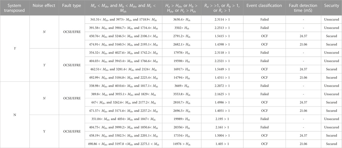
TABLE 6. Results of OCSE/EFRE fault detection, identification, and fault classification using the DWT-based algorithm for the considered transposed and un-transposed lines with and without noise effect.

The first two cases failed to detect the fault caused by small fault resistance values. Furthermore, the DWT-based algorithm takes more time to detect the fault than the proposed fault detection, identification, and classification schemes.

5.2.4 Simulation results: case 4

The proposed fault detection, identification, and classification schemes also examined faults, such as LIFs and HIFs, considering various locations, inception angles, and fault resistance values. In this case, the values of Clarke components for the investigated scenarios are shown in Table 7. As presented in this table, the proposed fault detection, identification, and fault classification schemes are accurately distinguished between LIFs and HIFs. The DWT-based algorithm was also examined for the same scenarios in this case. The values of (M_a, M_b, and M_c), (H_a, H_b, and H_c), and (R_a, R_b, and R_c) are calculated and presented in Table 8.

TABLE 7

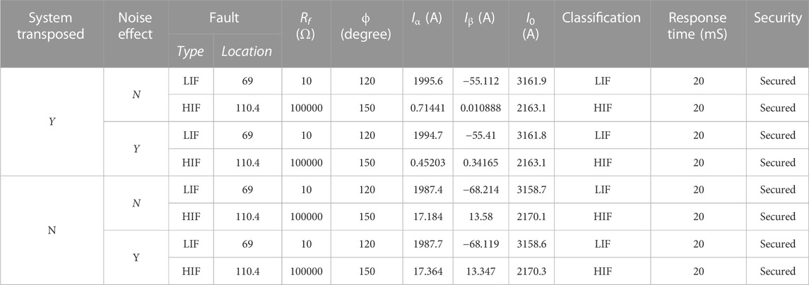
TABLE 7. LIF and HIF fault detection, identification, and fault classification results using the proposed schemes for the considered transposed and un-transposed lines with and without noise effect.

TABLE 8

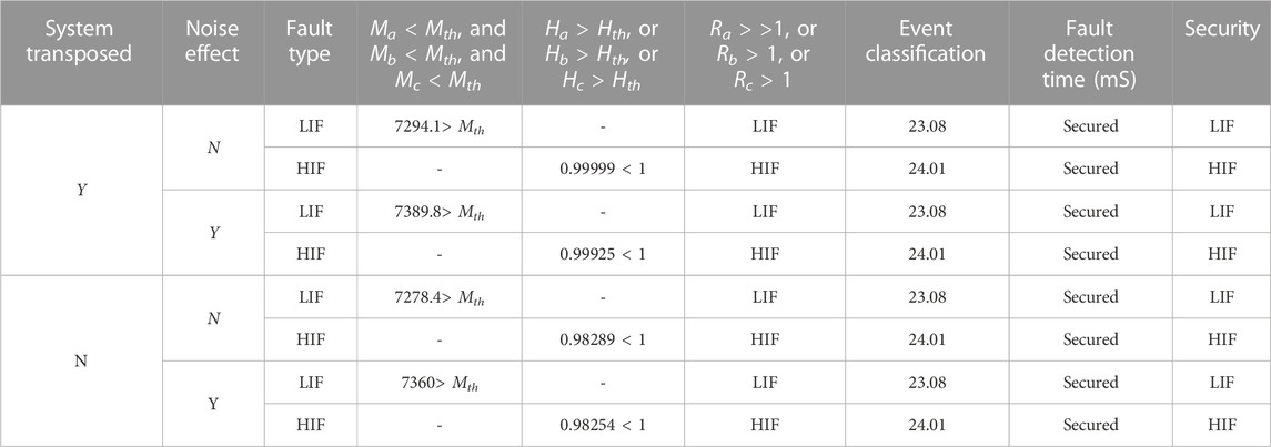
TABLE 8. LIF and HIF fault detection, identification, and fault classification results using the DWT-based algorithm for the considered transposed and un-transposed lines with and without noise effect.

The tables show that the DWT-based algorithm provided good discrimination between LIFs and HIFs. However, the DWT-based algorithm took considerable time for fault detection compared to the proposed fault detection, identification, and classification schemes.

5.3 Generalization of the proposed schemes

The proposed fault detection, identification, and fault classification schemes can also be generalized for any transmission system. Figure 14A shows the single-line diagram of 400 kV, 144 km TL simulated in the ATP/EMTP program. The ATPDraw software is an interface to implement the system (Prikler and Høidalen, 2009). This TL model is a benchmark in the ATPDraw software, and it is represented using the three-phase JMARTI frequency dependence model in the ATPDraw field using the line/cable module (Prikler and Høidalen, 2009). The JMARTI representation is a frequency-fitted model in a specific frequency range. The JMARTI model is utilized to apply the simulated line and, therefore, take waveforms for the fault case in evaluating the proposed schemes. For simultaneous series and shunt earth fault detection and classification using Clarke transform for TLs under different fault scenarios, the line parameters have been extracted, and results show that the self-impedance of this line, for a length of 144 km, is 0.3382 + j1.6009 Ω, while that of the mutually linked one is 0.3282 + j 0.8493 Ω, according to the retrieved line parameters. Using a mutually linked RL circuit, Thevenin’s equivalent impedance at buses S and R are expressed as R₁ = 1.0185 Ω and L₁ = 50.929 mH, and zero sequences are R₀ = 2.037 Ω, L₀= 101.85 mH at bus S and R₁ = 0.6366 Ω, L₁ = 31.83 mH, R₀= 1.2732 Ω, L₀= 63.66 mH at bus R. The TL configuration is illustrated in Figure 14B, where the dc resistance is 0.0522 Ω/km, and the outer diameter of the conductor is 3.18 cm. The sky wires are solid, their dc resistance is 0.36 Ω/mile, and the outer diameter is 1.46 cm. The resistivity of the soil is equal to 200 Ω. Similarly, a small error in simulation for 400 kV TL is found using system verification in the ATPDraw software program.

FIGURE 14

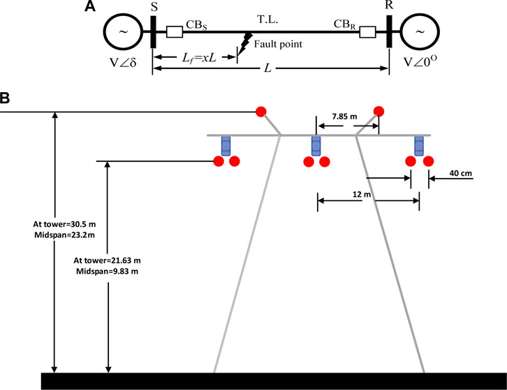
FIGURE 14. Single-line diagram of the second simulated TL system and the selected tower: (A) SLD; (B) tower configuration.

The proposed fault detection, identification, and classification schemes are also examined using another TL data, considering several fault types. In this case, the values of Clarke components for the investigated scenarios are shown in Table 9. In addition, the DWT-based algorithm was examined in the same scenarios, as shown in Table 10, where the values of (M_a, M_b, and M_c), (H_a, H_b, and H_c), and (R_a, R_b, R_c) were calculated. As presented in these tables, considering the OCRE/EFSE occurred, the values of M_a > M_th and M_c > M_th caused by small fault resistances were unmet. In addition, the values are H_a > H_th and R_a>1. Furthermore, the proposed fault detection, identification, and fault classification schemes provided precise fault detection, identification, and fault classification for the investigated types of faults.

TABLE 9

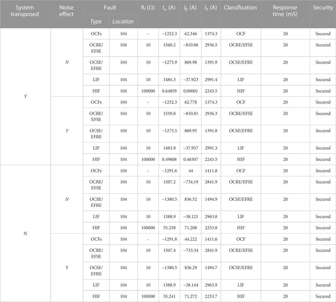
TABLE 9. Fault detection, identification, and fault classification results using the proposed schemes for the transposed and un-transposed lines with and without noise effect.

TABLE 10

TABLE 10. Fault detection, identification, and fault classification results using the DWT-based algorithm for transposed and un-transposed lines with and without noise effect.

The proposed schemes’ challenge is their performance if the current transformers’ saturation occurs. The current transformers must correctly provide the protection relays with the stepped-down fault current level. Proper means to detect current transformer saturation are essential for digital signal processing. Esmail et al. (2015) suggested an effective method for detecting current transformer saturation with a universal distinction index without a necessity for setting a definition. For this point, the instantaneous sample-based multiplication of the secondary current by its derivative is individually employed to distinguish between saturated and unsaturated wave portions.

Reconstructing the detected saturated secondary current is accomplished using Kalman filtering to obtain the phasor quantities of the unsaturated current portion professionally.

6 Conclusion

This study solves the challenge of detecting simultaneous earth faults in high-voltage transmission systems as traditional distance relays, for example, the inability to find or detect OCFs and simultaneous earth faults. The proposed schemes comprise two different stages: fault detection and identification and fault classification. The first proposed scheme needs communication links among both ends (sending and receiving) to detect and identify the fault. This communication link between both ends is used to send and receive three-phase currents’ magnitudes for sending and receiving ends in the proposed fault detection (PFD) unit at both ends. The second proposed scheme starts with proposed fault classification (PFC) units at both ends. The proposed classification technique applies the Clarke transform on local current signals to classify the open conductor and simultaneous faults. The sign of all current Clarke components is the primary key for distinguishing between all types of simultaneous LIFs and HIFs. Numerous simulation tests were investigated to analyze the performance of the suggested fault detection, identification, and classification schemes. In all scenarios, the fault type was accurately detected, identified, and classified within 20 mS after fault occurrence.

The security of the proposed schemes was also verified with different fault resistance values, and the suggested scheme provided precise fault detection, identification, and classification. The results demonstrated that fault detection, identification, and classification schemes are immune to fault types, locations, and inception angles. Furthermore, the suggested schemes detected both instants of the open conductor and down conductor. The developed scheme’s superiority was also validated through a comparison study with another published procedure based on discrete wavelet transform. No sophisticated artificial intelligence techniques were required to detect, identify, and classify the faults accurately. Also, the proposed fault detection, identification, and fault classification schemes have low mathematical requirements. It should be mentioned that the Clarke transform was used with a low sampling frequency in this work; hence, the suggested fault detection, identification, and classification approaches are guaranteed to be promising schemes that can be implemented in practice. Finally, other applications of the proposed schemes in series compensated transmission lines will be investigated in future works.

Data availability statement

The original contributions presented in the study are included in the article/Supplementary Material; further inquiries can be directed to the corresponding author.

Author contributions

Conceptualization: EE and FA; software: MC, EE, FA, and SA; validation: AA, AY, and AE-S; formal analysis: EE and FA; investigation: EE and AA; resources: SA; writing—original draft preparation: EE and SA; writing—review and editing: FA and SA; visualization: EE and AE-S. All authors contributed to the article and approved the submitted version.

Acknowledgments

This work was supported by the Researchers Supporting Project (RSPD 2023R646), King Saud University, Riyadh, Saudi Arabia.

Conflict of interest

The authors declare that the research was conducted in the absence of any commercial or financial relationships that could be construed as a potential conflict of interest.

Publisher’s note

All claims expressed in this article are solely those of the authors and do not necessarily represent those of their affiliated organizations, or those of the publisher, the editors, and the reviewers. Any product that may be evaluated in this article, or claim that may be made by its manufacturer, is not guaranteed or endorsed by the publisher.

Abbreviations

ATP/EMTP, alternative transient program/electromagnetic transient program; ATP, alternative transient program; TLs, transmission lines; OC, open conductor; OCFs, open conductor faults; OCRE/EFSE, OCFs at the receiving end followed by earth fault in the sending end; OCSE/EFRE, OC at the sending end followed by earth fault in the receiving end; LIFs, low-impedance faults; HIFs, high-impedance faults; DFT, discrete Fourier transform; PFD, proposed fault detection; PFC, proposed fault classification; DWT, discrete wavelet transform.

References

Abd-Elhamed Rashad, B., Ibrahim, D. K., Gilany, M. I., and El’Gharably, A. F. (2020). Adaptive single-end transient-based scheme for detection and location of open conductor faults in HV transmission lines. Electr. Power Syst. Res. 182, 106252. doi:10.1016/j.epsr.2020.106252

CrossRef Full Text | Google Scholar

Abdel-Aziz, A., Hasaneen, B. M., and Dawood, A. A. (2017). Detection and classification of one conductor open faults in parallel transmission line using artificial neural network. Int. J. Sci. Res. Eng. Trends. https://api.semanticscholar.org/CorpusID:28122028.

Google Scholar

Adewole, A. C., Rajapakse, A., Ouellette, D., and Forsyth, P. (2020). Residual current-based method for open phase detection in radial and multi-source power systems. Int. J. Electr. Power Energy Syst. 117, 105610. doi:10.1016/j.ijepes.2019.105610

CrossRef Full Text | Google Scholar

Alstom, G. (2017). “Network protection and automation guide: protective relays,” in Meas. Control. Retrieved 9th Febr.

Google Scholar

Ashok, V., Yadav, A., and Abdelaziz, A. Y. (2019). MODWT-based fault detection and classification scheme for cross-country and evolving faults. Electr. Power Syst. Res. 175, 105897. doi:10.1016/j.epsr.2019.105897

CrossRef Full Text | Google Scholar

Assadi, K., Slimane, J. B., Chalandi, H., and Salhi, S. (2023). Shunt faults detection and classification in electrical power transmission line systems based on artificial neural networks. COMPEL - Int. J. Comput. Math. Electr. Electron. Eng. ahead-of-print. doi:10.1108/COMPEL-10-2022-0371

CrossRef Full Text | Google Scholar

Asuhaimi Mohd Zin, A., Saini, M., Mustafa, M. W., Sultan, A. R., and Rahimuddin, (2015). New algorithm for detection and fault classification on parallel transmission line using DWT and BPNN based on Clarke’s transformation. Neurocomputing 168, 983–993. doi:10.1016/j.neucom.2015.05.026

CrossRef Full Text | Google Scholar

Banner, C. L., and Don Russell, B. (1997). Practical high-impedance fault detection on distribution feeders. IEEE Trans. Ind. Appl. 33, 635–640. doi:10.1109/28.585852

CrossRef Full Text | Google Scholar

Bañuelos-Cabral, E. S., Gutiérrez-Robles, J. A., García-Sánchez, J. L., Sotelo-Castañón, J., and Galván-Sánchez, V. A. (2019). Accuracy enhancement of the JMarti model by using real poles through vector fitting. Electr. Eng. 101, 635–646. doi:10.1007/s00202-019-00807-8

CrossRef Full Text | Google Scholar

Dash, P. K., Pradhan, A. K., and Panda, G. (2000). A novel fuzzy neural network based distance relaying scheme. IEEE Trans. Power Deliv. 15, 902–907. doi:10.1109/61.871350

CrossRef Full Text | Google Scholar

Elkalashy, N. I., Kawady, T. A., Khater, W. M., and Taalab, A.-M. I. (2016). Unsynchronized Fault-location technique for double-circuit transmission systems independent of line parameters. IEEE Trans. Power Deliv. 31, 1591–1600. doi:10.1109/TPWRD.2015.2472638

CrossRef Full Text | Google Scholar

Elkalashy, N. I. (2014). Simplified parameter-less fault locator using double-end synchronized data for overhead transmission lines. Int. Trans. Electr. Energy Syst. 24, 808–818. doi:10.1002/etep.1736

CrossRef Full Text | Google Scholar

Elmitwally, A., and Ghanem, A. (2021). Local current-based method for fault identification and location on series capacitor-compensated transmission line with different configurations. Int. J. Electr. Power Energy Syst. 133, 107283. doi:10.1016/j.ijepes.2021.107283

CrossRef Full Text | Google Scholar

Esmail, E. M., Elkalashy, N. I., Kawady, T. A., Taalab, A.-M. I., and Lehtonen, M. (2015). Detection of partial saturation and waveform compensation of current transformers. IEEE Trans. Power Deliv. 30, 1620–1622. doi:10.1109/TPWRD.2014.2361032

CrossRef Full Text | Google Scholar

Esmail, E. M., Elgamasy, M. M., Kawady, T. A., Taalab, A.-M. I., Elkalashy, N. I., and Elsadd, M. A. (2022). Detection and experimental investigation of open conductor and single-phase earth return faults in distribution systems. Int. J. Electr. Power Energy Syst. 140, 108089. doi:10.1016/j.ijepes.2022.108089

CrossRef Full Text | Google Scholar

Ghaderi, A., Ginn, H. L., and Mohammadpour, H. A. (2017). High impedance fault detection: A review. Electr. Power Syst. Res. 143, 376–388. doi:10.1016/j.epsr.2016.10.021

CrossRef Full Text | Google Scholar

Gilany, M., Al-Kandari, A., and Hassan, B. (2010). “ANN based technique for enhancement of distance relay performance against open-conductor in HV transmission lines,” in 2010 The 2nd International Conference on Computer and Automation Engineering, Singapore, 26-28 February 2010 (ICCAE), 50–54.

CrossRef Full Text | Google Scholar

Jayabharata Reddy, M., and Mohanta, D. K. (2007). A wavelet-fuzzy combined approach for classification and location of transmission line faults. Int. J. Electr. Power Energy Syst. 29, 669–678. doi:10.1016/j.ijepes.2007.05.001

CrossRef Full Text | Google Scholar

Jayamaha, D. K. J. S., Madhushani, I. H. N., Gamage, R. S. S. J., Tennakoon, P. P. B., Lucas, J. R., and Jayatunga, U. (2017). “Open conductor fault detection,” in 2017 Moratuwa Engineering Research Conference, Moratuwa, Sri Lanka, 29-31 May 2017 (MERCon), 363–367.

CrossRef Full Text | Google Scholar

Jeerings, D. I., and Linders, J. R. (1991). A practical protective relay for down-conductor faults. IEEE Power Eng. Rev. 11, 59. doi:10.1109/MPER.1991.88840

CrossRef Full Text | Google Scholar

Kavaskar, S., and Kant, N. (2019). Detection of high impedance fault in distribution networks. Ain Shams Eng. J. 10, 5–13. doi:10.1016/j.asej.2018.04.006

CrossRef Full Text | Google Scholar

Khoshbouy, M., Yazdaninejadi, A., and Bolandi, T. G. (2022). Transmission line adaptive protection scheme: A new fault detection approach based on pilot superimposed impedance. Int. J. Electr. Power Energy Syst. 137, 107826. doi:10.1016/j.ijepes.2021.107826

CrossRef Full Text | Google Scholar

Koley, E., Yadav, A., and Thoke, S. A., (2014). Artificial neural network based protection scheme for one conductor open faults in six phase transmission line. Int. J. Comput. Appl. 101, 42–46. doi:10.5120/17678-8522

CrossRef Full Text | Google Scholar

Mahanty, R. N., and Gupta, P. B. D. (2007). A fuzzy logic based fault classification approach using current samples only. Electr. Power Syst. Res. 77, 501–507. doi:10.1016/j.epsr.2006.04.009

CrossRef Full Text | Google Scholar

Prikler, L., and Høidalen, H. K. (2009). For windows 9x/NT/2000/XP/vista users ’ manual.

Google Scholar

Rathore, B., and Shaik, A. G. (2015). “Fault detection and classification on transmission line using wavelet based alienation algorithm,” in 2015 IEEE Innovative Smart Grid Technologies - Asia (ISGT ASIA), Bangkok, Thailand, 03-06 November 2015, 1–6.

CrossRef Full Text | Google Scholar

Saravanababu, K., Balakrishnan, P., and Sathiyasekar, K. (2013). “Transmission line faults detection, classification, and location using Discrete Wavelet Transform,” in 2013 International Conference on Power, Energy and Control, Dindigul, India, 6-8 February 2013 (ICPEC), 233–238.

CrossRef Full Text | Google Scholar

Shaik, A. G., and Pulipaka, R. R. V. (2015). A new wavelet based fault detection, classification and location in transmission lines. Int. J. Electr. Power Energy Syst. 64, 35–40. doi:10.1016/j.ijepes.2014.06.065

CrossRef Full Text | Google Scholar

Shukla, S. K., Koley, E., and Ghosh, S. (2017). “Detection and classification of open conductor faults in six-phase transmission line using wavelet transform and naive Bayes classifier,” in 2017 IEEE International Conference on Computational Intelligence and Computing Research, Coimbatore, India, 14-16 December 2017 (ICCIC), 1–6.

CrossRef Full Text | Google Scholar

Silva, S., Costa, P., Gouvea, M., Lacerda, A., Alves, F., and Leite, D. (2018). High impedance fault detection in power distribution systems using wavelet transform and evolving neural network. Electr. Power Syst. Res. 154, 474–483. doi:10.1016/j.epsr.2017.08.039

CrossRef Full Text | Google Scholar

Usama, Y., Lu, X., Imam, H., Sen, C., and Kar, N. C. (2014). Design and implementation of a wavelet analysisbased shunt fault detection and identification module for transmission lines application. IET Gener. Transm. Distrib. 8, 431–441. doi:10.1049/iet-gtd.2013.0200

CrossRef Full Text | Google Scholar

Velez, F. (2014). “Open conductor analysis and detection,” in 2014 IEEE PES General Meeting | Conference and Exposition, Dallas, Texas, United States, July 2014, 1–7.

CrossRef Full Text | Google Scholar

Vieira, F. L., Santos, P. H. M., Carvalho Filho, J. M., Leborgne, R. C., and Leite, M. P. (2019). A voltage-based approach for series high impedance Fault Detection and location in distribution systems using Smart meters. Energies 12, 3022. doi:10.3390/en12153022

CrossRef Full Text | Google Scholar

Zanjani, M. G. M., Kargar, H. K., and Zanjani, M. G. M. (2012). “High impedance fault detection of distribution network by phasor measurement units,” in 2012 Proceedings of 17th Conference on Electrical Power Distribution, Tehran, Iran, 2-3 May 2012, 1–5.

Google Scholar