TCN-GAT multivariate load forecasting model based on SHAP value selection strategy in integrated energy system

1 Introduction

In order to promote the achievement of the “dual carbon” goal and support China’s ecological civilization construction and sustainable development, it is necessary to build a clean, low-carbon, safe and efficient energy system (Zhang et al., 2023). The planning, design, and operation of traditional energy subsystems are often separated from each other. The coupling between different types of energy is not well reflected, leading to a decline in energy utilization and safety performance. Integrated energy system (IES) is a new energy system that integrates power, refrigeration, heating and other energy supplies (Ren et al., 2020; Chen et al., 2021). It can realize the conversion, utilization, coordinated optimization and coupling complementarity of multiple energies such as electricity, cooling, heat and gas. As the physical carrier of the energy internet, IES can meet the diversified energy demand of the economy and society (Yang et al., 2010), while improving the energy supply reliability and comprehensive utilization of the system, reducing energy costs and carbon emissions, and promoting high-quality development of the energy industry. Facing the complex and diversified energy supply coupling mechanism in IES, it is necessary to accurately forecast the energy loads to ensure the rational planning and safe operation of the energy system.

For the multivariate load forecasting problem in the integrated energy system, two main methods are currently used: traditional time series data analysis and machine learning (Sun et al., 2021; Wang et al., 2022). In the face of one single load forecasting, traditional methods such as vector autoregressive model (VAR) and autoregressive integrated moving average model (ARIMA) are mostly chosen (Yuan et al., 2017; Yang et al., 2018). These methods only consider the variation law of one load, and do not correspond to an effective adaptation mechanism for the coupling characteristics of multivariate loads. Currently, forecasting models based on machine learning are gradually applied in multivariate load forecasting studies, such as general regression neural networks (GRNN) (Li et al., 2018; Zhu, 2020), support vector regression (SVR) (Fan et al., 2017), extreme learning machine (Liu et al., 2015), etc. Compared with traditional methods, these models have achieved certain results in multivariate forecasting. However, with the development of new energy resources, the proportion of renewable energy access and the complexity of user-side energy demand are increasing, which deepens the features and dimensions of the energy database. It is difficult to construct an accurate and effective algorithm structure to simulate the actual energy supply system and energy demand response, so the forecasting accuracy needs to be improved. In recent years, deep learning has been more and more widely used in the study of time series forecasting, among which typical models are represented by long short-term memory neural networks (LSTM) (Wang et al., 2019; Wang et al., 2020), convolutional neural networks (CNN) (Liu et al., 2019), recurrent neural networks (RNN) (Sfetsos, 2000), etc. Li et al. (2020) utilize multi-column convolutional neural networks (MCNN) for independent extraction and unified fusion of features of two-dimensional load pixels in high-dimensional space, and input the combined features into LSTM for load forecasting. Li et al. (2022) develop a combined model based on the convolutional neural network and gated recurrent unit. According to the model structure adjustment strategy based on the maximum mean difference, the model structure was dynamically adjusted to the complex prediction environment.

The above deep learning models have been validated for data mining and feature learning capability of time series, but they have their own limitations. These models can not achieve deep mining and optimal expression in the face of complex correlations among multiple energy loads. It has been documented that combining multi-task learning (MTL) with neural networks has certain advantages in multivariate load forecasting (Tan et al., 2020; Wu C et al., 2022). However, related studies only simply “hard-connect” them without reflecting that each feature variable has a different influence and contribution to different subtasks.

In addition, we have investigated some new methods for time series learning. Qin et al. (2022) introduce the LSTM mechanism into Capsule Network (CapsNet) to capture long-term temporal correlation of run-to-failure time series measured from degraded mechanical equipment for accurate RUL estimation. The results show that CapsNet outperforms CNN in image-based inference tasks, but whether it retains its superiority in the forecasting of multivariate loads remains to be investigated. Gaugel and Reichert. (2023) adopt the transfer learning method to pre-train deep learning network in the case of scarce industrial data. The results demonstrate that transfer learning can enhance the performance of time series segmentation models with respect to accuracy and training speed. However, in the scenario of non-related datasets, cases of negative transfer learning were observed as well. Therefore, it is a difficult task to find which dataset is more relevant.

The temporal convolutional network (TCN) is a neural network model that utilizes causal convolution and dilated convolution, which can perform convolution in parallel (Bai et al., 2018). When the input sequence is long and multi-dimensional, the gradients in TCN are more stable and occupy less memory compared with other models, which gives the network a faster processing speed and deeper information mining capability when facing multivariate load forecasting problems. The SHAP (Shapley Additive Explanation) method is a game-theoretic-based additive feature attribution method that can be used for local and global interpretation of arbitrary models (Wu K. L et al., 2022). There is a lot of redundant information in the training process of deep learning algorithms. The SHAP method is chosen to provide global interpretation, which can reveal the relationship between different feature variables and forecasting results. Meanwhile, it can measure the influence of these features on each subtask, so as to filter out the effective features of the data. The global attention model (GAT) is also used to weigh the useful information in TCN and suppress useless information in this paper. The combination of the above methods can efficiently process complex and correlated multi-dimensional time series load data and is adapted to the interpretability study of the multivariate load forecasting model.

Considering the characteristics of strong interaction and coupling among multiple energy sources in integrated energy systems, a TCN-GAT multivariate load forecasting model based on SHAP value selection strategy is proposed in this paper. The multivariate load data in IES with related influencing factors are input into the TCN network, and the global attention mechanism is applied to the hidden layer state of the network. The SHAP values of the feature variables in the multivariate load forecasting task are calculated by global samples. The features that contribute more to the forecasting results are selected as input variables, and then returned to the TCN-GAT model for training and learning to obtain load forecasting results. This forecasting model can quantify the different correlations of each load-influencing factor in a weighted manner, thus achieving the purpose of decoupling and analyzing complex coupled data for accurate and efficient forecasting. Finally, it is verified by practical examples that the multivariate load forecasting model proposed in this paper has better learning ability and forecasting performance.

2 IES characteristics and SHAP method

2.1 Analysis of sub-energy characteristics in IES

The integrated energy system (IES) is an energy balance system that integrates multiple energy sources in a certain area through advanced physical information technology and innovative management models to achieve a highly coordinated “source-grid-load” system (Tan et al., 2020). Compared with the traditional energy system, the integrated energy system has various characteristics such as cross-complementary energy sources, improved reliability and economy of energy supply, and facilitation of large-scale renewable energy consumption. The internal energy flow relationship of IES is shown in Figure 1.

FIGURE 1

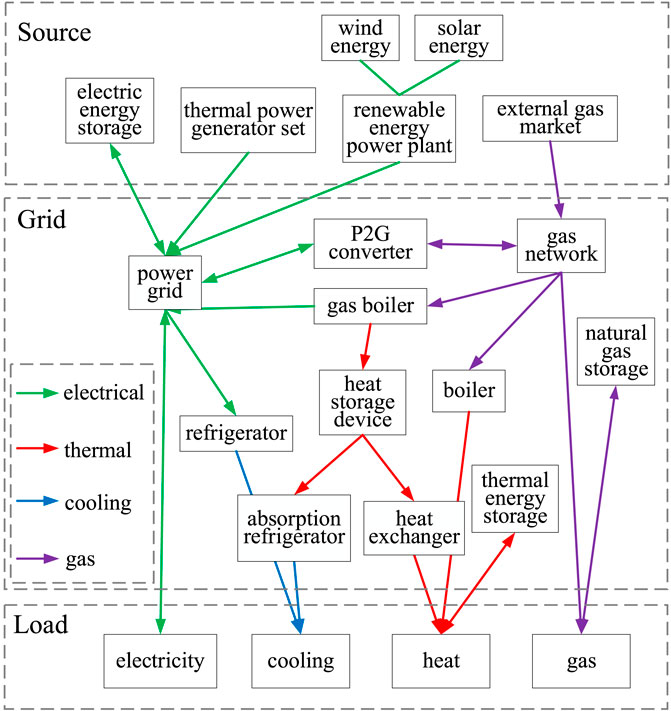
FIGURE 1. Energy flow relationships among subsystems of IES.

The subsystems of IES have certain independence and interaction according to its operation characteristics and transformation laws in energy production and consumption, in order to meet the load demand on the user side. As can be seen from Figure 1, IES consists of electrical energy system, cooling energy system, thermal energy system and gas energy system. It operates according to the mutual demand and energy conversion production law among electricity, cooling, heat and gas loads, so the multiple energy forms in IES are in a state of simultaneous coupling. In addition, the types of energy input into IES include wind and solar energy, which are susceptible to environmental changes. So external environmental factors also have an influential role in the IES load changes.

Multivariate load forecasting for integrated energy systems can help achieve coordinated planning, interactive response and optimal operation among multiple energy subsystems. The energy coupling characteristic of IES determines that changes in one type of energy demand will inevitably cause service providers to adjust the other types of energy demand. Due to the complex structure of IES, the amount of data accumulated in long-term operation is sufficient and huge, so it is difficult to carry out simulation directly. Therefore, this paper selects the deep learning method for analysis, adopts TCN neural network to mine deep feature information in the data, captures useful information in the training process with the help of global attention mechanism, calculates SHAP values for input variables filtering, and ultimately completes the multivariate load forecasting task in IES.

2.2 SHAP method

SHAP (Shapley Additive Explanation) is a game theory-based additive feature attribution method proposed by Lundberg (Lundberg and Lee, 2017), which regards all input features in machine learning as “contributors”. It quantifies the relationship between input features and output results by calculating the contribution of each feature to the forecasting sample. The specific expression is as follows:

${\mathit{y}}_{\mathit{i}}={\mathit{y}}_{\mathit{b}\mathit{a}\mathit{s}\mathit{e}}+\mathit{f}\left({\mathit{x}}_{\mathit{i}\mathbf{1}}\right)+\mathit{f}\left({\mathit{x}}_{\mathit{i}\mathbf{2}}\right)+\cdots +\mathit{f}\left({\mathit{x}}_{\mathit{i}\mathit{n}}\right)(1)$

where y_i is the prediction value of the model for sample x_i, y_base is the mean value of the sum of all sample predictions, and f (x_i1) is the contribution value of the first feature in the ith sample to the final forecasting result. When f (x_i1) > 1 indicates that the feature has a positive effect on the prediction of the target value; otherwise, it has a negative effect. Therefore, the SHAP value can not only show the magnitude of feature influence, but also reflect the positivity or negativity of feature influence in each sample.

The SHAP method can be used for local and global interpretation of arbitrary models. The core idea is to calculate the marginal contribution of the features to the model output, and then interpret the “black box model” at both local and global levels. Since it is necessary to simultaneously forecast the future moment values of electricity, cooling and heat loads in an integrated energy system, and analyze the contribution of input feature variables to the forecasting results, this paper adopts an input variable selection strategy based on SHAP values, as shown in Figure 2. The SHAP values of the feature variables in the multivariate load forecasting task are calculated by global samples, and only the features that contribute more to the forecasting results are selected as input variables to improve the accuracy and effectiveness of the forecasting model.

FIGURE 2

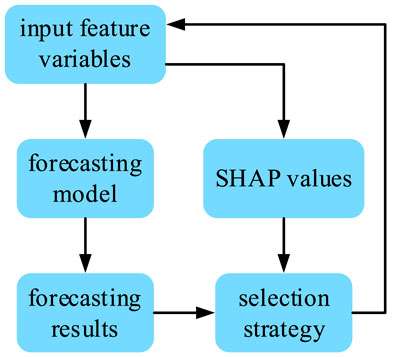
FIGURE 2. Input variable selection strategy based on SHAP values.

The core of introducing SHAP value calculation into multivariate coupling variable forecasting is to interpret the model forecasting results as a linear function of binary variables. Assuming that the input variable vector of the forecasting model is x = (x₁, x₂, … , x_n), where n is the number of input variables. Then the global interpretation model based on SHAP values can be expressed on the basis of the original multivariate load forecasting model as follows:

$\mathit{f}\left(\mathit{x}\right)=\mathit{g}\left({\mathit{x}}^{\prime }\right)={\mathit{\phi }}_{\mathbf{0}}+{\displaystyle \sum _{\mathit{i}=\mathbf{1}}^{\mathit{n}}}{\mathit{\phi }}_{\mathit{i}}{{\mathit{x}}_{\mathit{i}}}^{\prime }(2)$

where f(x) is the output of the multivariate load forecasting model, g (x') is the output of the interpretation model, ${\phi }_0$ is the forecasting reference value, generally the average of the forecasting results, ${\phi }_i$ is the SHAP value of the ith feature, and ${x_i}^{\prime }\in {\left\{\mathrm{0,1}\right\}}^n$ is the binary mapping variable of the input feature, representing the presence or absence of the ith feature in that sample.

The input variable selection strategy based on SHAP values is introduced to fit the load forecasting model as an interpretable linear model. The contribution of each feature to the load forecasting results can be obtained by calculating the SHAP values of each feature variable in the global sample. The features with smaller contributions are screened out to improve the multivariate load forecasting performance.

3 TCN network and GAT mechanism

3.1 Temporal convolutional network

At present, the recurrent neural network architecture in the context of deep learning is mainly used for forecasting integrated energy loads, such as LSTM network, GRU network (Ye et al., 2022), etc. Bai et al. (2018) believe that there exists a neural network model that utilizes causal convolution and dilated convolution when modeling time series data, namely, temporal convolutional network (TCN). It can improve model performance and avoid problems such as gradient disappearance, explosion or lack of memory retention in recursive models. So it is adapted to modeling tasks of time series.

When training a temporal convolutional network, the value at time t of the previous layer only depends on the value at and before time t of the next layer, which means TCN is a strictly time-constrained model. Therefore, the TCN network has two main constraints: the output and input should have the same length, and the network should only use information from past steps. To satisfy these temporal principles, a one-dimensional fully convolutional network structure (1D FCN) is used in TCN, where each hidden layer has the same length as the input layer, and zero-padding is used to ensure that subsequent layers have the same length. In addition, for the network output, TCN uses causal convolution, which means the output of each layer at time step t is no later than the region at the same time step of the previous layer.

When dealing with time series, the network is expected to retain long-term information. However, pure causal convolution still has the problem of traditional convolution neural networks, that is, the length of time modeling is limited by the size of the convolution kernel. In order to capture longer-term relevant information, it is necessary to stack many layers linearly. So the researchers proposed the concept of dilated convolution. Figure 3 shows a schematic diagram of causal and dilated convolution.

FIGURE 3

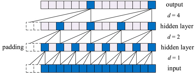
FIGURE 3. Causal and dilated convolution with expansion factor d = 1, 2, 4.

Different from traditional convolution, the dilated convolution allows the input to be sampled at intervals during convolution, and the sampling rate is controlled by d in Figure 3, which is the dilated exaggeration factor. The lowest layer d = 1, indicating that every point is sampled as input. The middle layer d = 2, indicating that one of every two points is sampled as input. And so on. In general, the higher the layer, the larger the d used, thus achieving a finite layer network with exponentially sized receptive fields. Therefore, the TCN uses dilated convolution to obtain input from every d steps at time t: x_t-(k-1)d, … , x_t-2d, x_t-d, x_t, where k is the kernel size. Dilated convolution allows the network to go back (k-1)d time steps before, allowing the receptive field of each layer to grow exponentially.

The residual connection proves to be an effective method for training deep networks. It enables the network to transfer information in a cross-layer manner, thus obtaining a sufficiently large receptive field. It not only speeds up the training process, but also avoids the gradient vanishing problem of deep models. The residual block constructed in this paper contains two layers of convolution and nonlinear mapping. To normalize the input of hidden layer, weight normalization is applied to each convolution layer to counteract the gradient explosion problem. To prevent overfitting, regularization is introduced through Dropout after the convolution layer of each residual block. Meanwhile, the ReLU activation function is added to the residual block after the two convolutional layers to introduce non-linearity to the TCN. Figure 4 shows the final residual block.

FIGURE 4

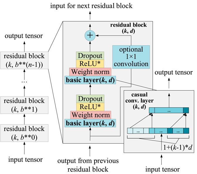
FIGURE 4. Residual block in TCN network.

3.2 Global attention model

The attention mechanism in deep learning draws on the human attention mindset. It has been widely used in various types of deep learning tasks, such as natural language processing, image classification and speech recognition, and has achieved remarkable results. The attention mechanism can flexibly capture the relationship between local and global samples. It observes the weight share of useful information, and thus pays more attention to the parts similar to the input elements and suppresses useless information.

The attention mechanism has been frequently used in machine translation processes in recent years (Bahdanau et al., 2014). In this process, Luong et al. (2015) proposed an effective attention model: the global attention model (GAT). The model structure diagram is shown in Figure 5.

FIGURE 5

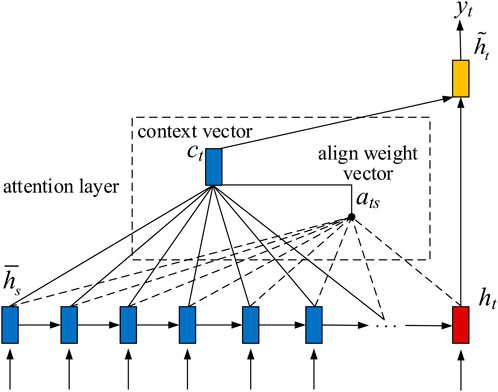
FIGURE 5. Structure diagram of global attention model.

The global attention model is characterized by considering all hidden states of the encoder when deriving each context vector c_t. For each time step t, the model will derive a content-based score function according to the current hidden state h_t at the top layer of the neural network and all source states ${\overline{h}}_s$ as follows:

$\mathbf{s}\mathbf{c}\mathbf{o}\mathbf{r}\mathbf{e}\left({\mathit{h}}_{\mathit{t}},{\overline{\mathit{h}}}_{\mathit{s}}\right)={\mathit{h}}_{\mathit{t}}^{\mathit{T}}{\mathit{W}}_{\mathit{a}}{\overline{\mathit{h}}}_{\mathit{s}}(3)$

where W_a represents the weight of each source state. By comparing the current target hidden state h_t with the source hidden state ${\overline{h}}_s$, a variable-length alignment vector a_ts can be obtained. a_ts represents the attention weight of each ${\overline{h}}_s$, whose size equals the number of time steps on the source side:

${\mathit{a}}_{\mathit{t}\mathit{s}}=\frac{\mathbf{exp}\left(\mathbf{s}\mathbf{c}\mathbf{o}\mathbf{r}\mathbf{e}\left({\mathit{h}}_{\mathit{t}},{\overline{\mathit{h}}}_{\mathit{s}}\right)\right)}{{\sum }_{{\mathit{s}}^{\prime }=\mathbf{1}}^{\mathit{S}}\mathbf{exp}\left(\mathbf{s}\mathbf{c}\mathbf{o}\mathbf{r}\mathbf{e}\left({\mathit{h}}_{\mathit{t}},{\overline{\mathit{h}}}_{{\mathit{s}}^{\prime }}\right)\right)}(4)$

Using all source states ${\overline{h}}_s$ of the neural network as input, with the alignment vector a_ts as the weight, a context vector c_t can be derived. It can capture relevant source-side information and help predict the current target y_t. c_t is calculated as the weighted average of all source hidden states:

${\mathit{c}}_{\mathit{t}}={\displaystyle \sum }_{\mathit{s}}{\mathit{a}}_{\mathit{t}\mathit{s}}{\overline{\mathit{h}}}_{\mathit{s}}(5)$

Here a simple concatenation layer is used to combine the information from both vectors, resulting in the following attentional vector:

${\stackrel{\sim }{\mathit{h}}}_{\mathit{t}}=\mathit{f}\left({\mathit{c}}_{\mathit{t}},{\mathit{h}}_{\mathit{t}}\right)=\mathbf{tanh}\left({\mathit{W}}_{\mathit{c}}\left[{\mathit{c}}_{\mathit{t}};{\mathit{h}}_{\mathit{t}}\right]\right)(6)$

Finally, the attention vector ${\stackrel{\sim }{h}}_t$ is fed through the softmax layer to produce the predictive distribution with the following formula:

$\mathit{p}\left({\mathit{y}}_{\mathit{t}}|\mathit{y}<\mathit{t},\mathit{x}\right)=\mathbf{s}\mathbf{o}\mathbf{f}\mathbf{t}\mathbf{m}\mathbf{a}\mathbf{x}\left({\mathit{W}}_{\mathit{s}}{\stackrel{\sim }{\mathit{h}}}_{\mathit{t}}\right)(7)$

The GAT model uses the hidden state at the top layer of the neural network in the encoder and decoder to predict the target y_t sequentially through the order: ${\overline{h}}_s$ →a_ts→c_t→ ${\stackrel{\sim }{h}}_t$. The calculation path is clear and convenient. By combining the GAT model with the TCN neural network, the feature parameters in the network input that have a greater impact on the results can be given greater weights, while reducing the weights of non-critical features that have a lower impact, so as to improve the accuracy and rationality of the load forecasting model.

4 Multivariate load forecasting model

4.1 TCN-GAT forecasting model

In this paper, a multivariate load forecasting model under the integrated energy system is constructed by combining TCN neural network and global attention mechanism. The structure diagram is shown in Figure 6. The time series data corresponding to the collected electricity, cooling, and heat loads with the relevant influencing feature parameters such as horizontal irradiance, air temperature, station pressure, humidity and so on are used as the input variables of the TCN network. The GAT mechanism is applied to the state output of the network hidden layer. In this case, the attention mechanism is manifested by using multiple concatenation layers to analyze the influence of different input feature parameters on the forecasting results, quantifying them into feature weight coefficients, and performing a weighted summation of the forecasting results of electricity, cooling and heat loads respectively. The key features affecting the load changes are highlighted, and the less relevant features are weakened, so as to achieve the purpose of internal decoupling and accurate calculation within the coupled multivariate load forecasting model. This paper uses the training set data to train and optimize the model, and calculates the loss function value. When the loss of the validation set reaches the minimum, output the optimal model, and input the test set data into the optimal TCN-GAT model for load forecasting analysis.

FIGURE 6

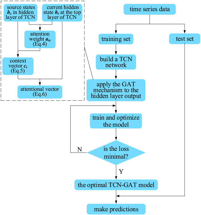
FIGURE 6. Structure diagram of TCN-GAT forecasting model.

4.2 Multivariate load forecasting model based on SHAP value selection strategy

Figure 7 illustrates the multivariate load forecasting model based on SHAP value selection strategy proposed in this paper. By inputting the multivariate load series data into the TCN-GAT model, the forecasting results of electricity, cooling and heat loads can be weighted and quantified according to the different correlations of their influencing factors, respectively. This paper filters the input variables by calculating SHAP values of each feature, and then return them to the TCN-GAT model for training and learning to obtain the multivariate load forecasting results. It can further reduce the forecasting error, remove the interference of low-correlation features on the model, thus improving the forecasting effect. Combining these two methods can effectively deal with complex and correlated multi-dimensional time series load data, and adapt to the interpretability study of multivariate load forecasting model.

FIGURE 7

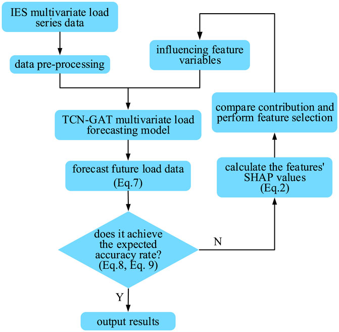
FIGURE 7. Structure diagram of multivariate load forecasting model based on SHAP value selection strategy.

The multivariate load forecasting model based on SHAP value selection strategy mainly follows the following four steps:

(1) Perform data pre-processing work such as gap data filling and anomaly data repair for the collected IES multivariate load series data, and initially determine the feature parameters affecting the load forecasting results.

(2) Input the time series data of electricity, cooling and heat loads and related feature parameters into the trained optimal TCN-GAT multivariate load forecasting model to forecast and analyze these load values in the future.

(3) Calculate the evaluation indexes of the forecasting results, and determine whether the expected accuracy is achieved. Output the final results if it is achieved, otherwise, proceed to the next step.

(4) Calculate the SHAP values of each feature and compare their contribution to the forecasting results. Filter out the features with less influence, keep the remaining input parameters, and return to step (2) again for load forecasting.

5 Case analysis

5.1 Data collection

In this paper, the electricity, cooling, and heat load data from Tempe campus of Arizona State University are used as experimental data (AUS, 2023). Environmental factors consider global horizontal irradiance, temperature, humidity, average wind speed, average wind direction (angle from N), and atmospheric pressure, in the Measurement and Instrumentation Data Center on the official website of the National Renewable Energy Laboratory (NREL) (NREL, 2023). The data are selected from the nearest meteorological station to the Tempe campus. The calendar rule considers weekday and holiday conditions. The data are collected for 2 years from 1 July 2011 to 1 July 2013, in 15-minite steps. The training set, validation set, and test set are divided into 7:2:1 intervals. The experiments are implemented in Tensorflow framework using Python language.

5.2 Evaluation indexes

Given that the constructed multivariate load forecasting model requires prediction and analysis of multiple load types at the same time, root mean square error (RMSE) and mean absolute percentage error (MAPE) are chosen as evaluation indexes in this paper. The specific expressions are as follows:

${\mathit{E}}_{\mathbf{R}\mathbf{M}\mathbf{S}\mathbf{E}}=\sqrt{\frac{{\displaystyle \sum _{\mathit{t}=\mathbf{1}}^{\mathit{n}}}{\left({\mathit{y}}_{\mathit{t}}-{\widehat{\mathit{y}}}_{\mathit{t}}\right)}^{\mathbf{2}}}{\mathit{n}}}(8)$

${\mathit{E}}_{\mathbf{M}\mathbf{A}\mathbf{P}\mathbf{E}}=\frac{\mathbf{1}}{\mathit{n}}{\displaystyle \sum _{\mathit{t}=\mathbf{1}}^{\mathit{n}}}\left|\frac{{\widehat{\mathit{y}}}_{\mathit{t}}-{\mathit{y}}_{\mathit{t}}}{{\mathit{y}}_{\mathit{t}}}\right|\times \mathbf{100}\%(9)$

where y_t is the actual value, ${\widehat{y}}_t$ is the predicted value, and n is the number of samples involved in the calculation.

5.3 Model parameters setting

The accuracy of model prediction is strongly correlated with its structural design and hyperparameter selection. To obtain the optimal structural parameters of the model in this paper, the grid search method is used here to determine the values of TCN network parameters, and the parameter values of the GAT model are determined by variable control method.

Experimentally, the number of convolutional kernels of the TCN network is set to 64, and the expansion list is [1, 2, 4, 8]. The causal network is chosen, the residual block is added to skip the connections, and the Dropout layer with a deactivation rate of 0.1 is added to prevent overfitting. Batch normalization is used in the residual block and ReLU is selected for the activation function. To solve the sparse gradient and noise problem in the network, Adam algorithm is selected for parameter adjustment and iteration, which can update the neural network weights iteratively based on the training data. The hyperparameters of the TCN network are set as shown in Table 1.

TABLE 1

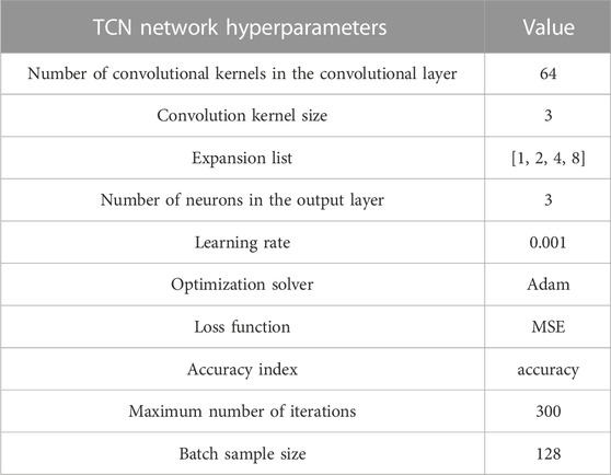
TABLE 1. TCN network hyperparameters.

The influence of neurons number in the Attention layer on the forecasting accuracy of the model is analyzed by several experiments, as shown in Table 2. According to its loss function value and model accuracy, the model training effect is best when the Attention layer is set to 16 neurons.

TABLE 2

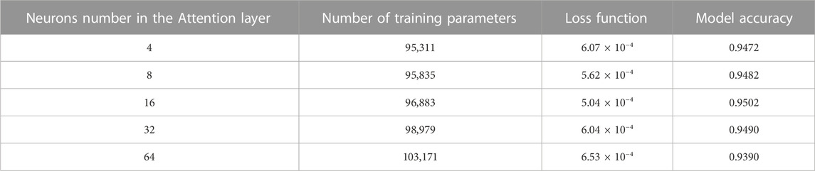
TABLE 2. The influence of neurons number in the Attention layer on the forecasting accuracy of the model.

Here adopts an early termination mechanism for the TCN-GAT model, which means the iterative training is stopped when the detection data do not improve for 30 consecutive training sessions. This not only ensures the generalization ability of the model by stopping training in time before the model falls into overfitting, but also prevents the model from underfitting due to too few training times.

5.4 Comparative analysis of forecasting results

5.4.1 Comparison of forecasting results based on SHAP value selection strategy

Perform load forecasting for 10-dimensional input features, including electricity load, cooling load, heat load, global horizontal irradiance, temperature, humidity, average wind speed, average wind direction, atmospheric pressure, and calendar rules, and calculate the global SHAP values of each feature. Here, the SHAP values of different features need to be obtained separately for the electricity, cooling and heat load forecasting results. Through the global interpretation of the SHAP method, the key characteristic parameters that affect different load changes can be more directly and clearly observed.

The global SHAP values of the 10-dimensional input features are arranged in descending order, as shown in Figure 8. Each point in the scatter plot represents a sample. The denser the sample, the wider the vertical width. The abscissa is the SHAP value. The sample points on the right side of the 0-axis indicate that the feature sample has a positive influence on the forecasting result, while the sample points on the left side indicate that the feature sample has a negative influence. The vertical axis represents the actual value of the sample itself. The redder the value, the larger the value. The bluer the value, the smaller the value.

FIGURE 8

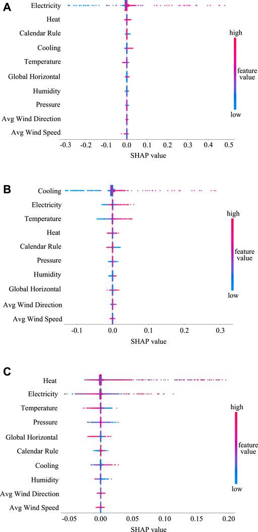
FIGURE 8. Diagrams of SHAP values of each feature on electricity load forecasting (A), cooling load forecasting (B) and heat load forecasting (C).

As can be seen from Figure 8 that each feature variable has different influences on the results of different forecasting tasks. Table 3 presents the contribution ranking of all the feature variables to the electricity, cooling and heat load forecasting results, from which the following conclusions can be drawn:

(1) The load forecasting task has a strong autocorrelation, that is, the load forecast value at a certain moment is closely related to its historical data before that moment. The autocorrelation of the electricity load is particularly obvious. This indicates that there is a certain internal regularity and continuity of each load series in the continuous time range.

(2) There is a strong correlation among electricity, cooling, and heat loads. This is because the measurement area is a campus environment, where cooling and heat demand is usually accompanied by an increase in electricity load. This also verifies the characteristics of the mutual coupling and correlation of energy within IES as described in the previous section, and proves the superiority of the multivariate load forecasting model proposed in this paper.

(3) There is a strong correlation between multivariate loads and external influencing factors. It can be seen from Figure 8 that these feature variables have a non-negligible effect on the three types of load forecasting results in this model. Since this paper establishes an integrated forecasting model for multiple loads, the input variables cannot be changed according to the individual forecasted load. Therefore, seven feature variables with the highest contribution to the forecasting results are selected here, which are electricity load, cooling load, heat load, temperature, global horizontal irradiance, calendar rule, and atmospheric pressure.

TABLE 3

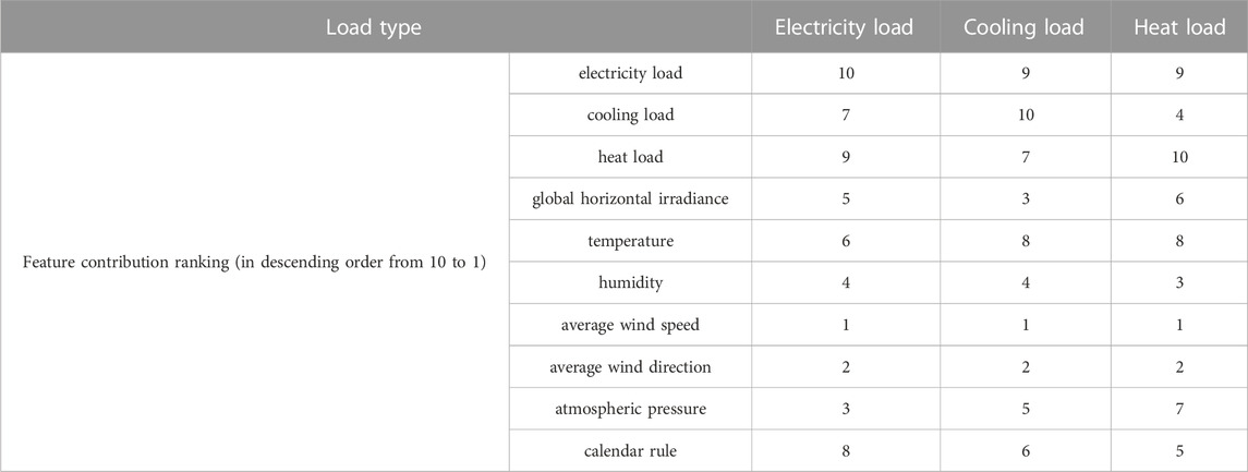
TABLE 3. Model input features filtered based on SHAP values.

The feature variables that have been selected by SHAP values are input into the model again for forecasting. The evaluation indexes of the two forecasting results are shown in Table 4. It is obvious that the forecasting error is reduced, indicating that the forecasting accuracy of the model is significantly improved after filtering the input features, which proves the effectiveness of the input feature selection strategy based on SHAP values.

TABLE 4

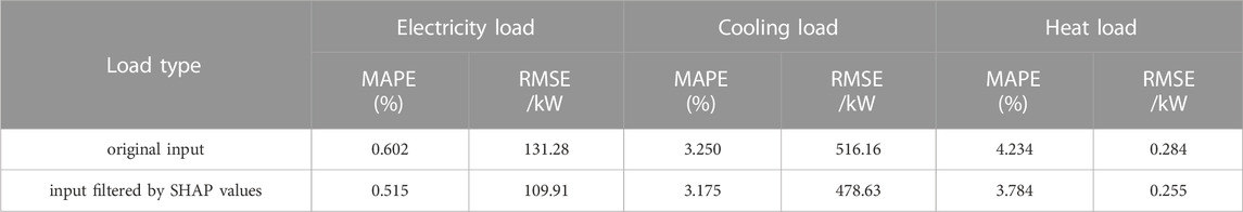
TABLE 4. Comparison of model forecasting effects based on SHAP value selection strategy.

5.4.2 Comparison of forecasting results of different models

To verify the accuracy and effectiveness of the TCN-GAT model for multivariate load data forecasting, the model proposed in this paper is compared with the other four forecasting models. The comparison models are: the LSTM neural network model, which is widely used in the load forecasting analysis of integrated energy systems, the LSTM-GAT model, the TCN neural network model, and the TCN-AT model, which combines the ordinary attention mechanism with the TCN network. The experimental forecasting results and evaluation indexes of different models are shown in Figure 9 and Table 5.

FIGURE 9

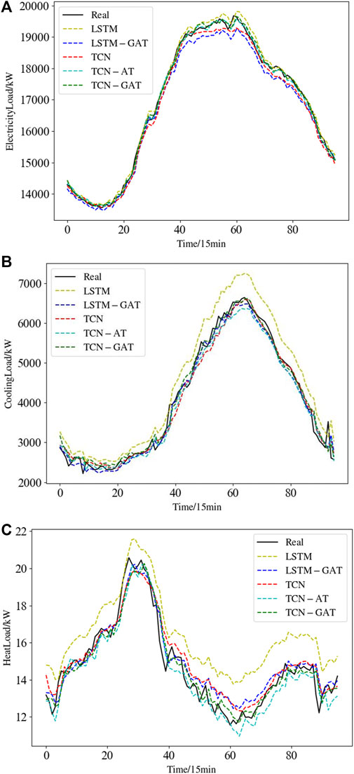
FIGURE 9. Model forecasting of a typical day on electricity load (A), cooling load (B) and heat load (C).

TABLE 5

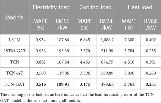
TABLE 5. Evaluation indexes of forecasting results of different models.

The forecasting results for different loads show that the electricity load has the highest forecasting accuracy, with an average E_MAPE of 3.544% lower compared to the cooling load and 3.9102% lower compared to the heat load. This is due to the fact that user’s electricity load is the most regular in time dimension and less affected by external climatic factors and calendar rules, which can be accurately predicted based on historical time series data through the deep information mining capability and historical behavior learning ability of TCN network. The cooling load forecasting error is smaller than that of the heat load, which is related to the environmental factors in the data collection area. Arizona State University is in a tropical desert climate with high temperature and dryness all year round. The cooling load demand is significantly higher than the heat load, so the prediction is more accurate and effective by learning the correlation information of the cooling load. While the heat demand in this area is low, the annual average heat load is 4.042 kW according to the original data collection. Observing E_RMSE, it can be seen that the heat load supply is low and the error is around 0.251 kW–0.402 kW, which accounts for a large proportion of the original load. Therefore, the final mean absolute error of heat load is the largest, and the forecasting accuracy is relatively the lowest.

Figure 9 shows the comparative analysis of the forecasting values of each model on a typical day. It can be seen that the forecasting errors of both LSTM and LSTM-GAT models are larger than those of TCN and TCN-GAT models. This indicates that the TCN network is superior to the LSTM network in terms of the integrated forecasting and learning ability for multivariate loads. The TCN-AT model has higher forecasting accuracy compared with the TCN network alone, and its E_MAPE for electricity, cooling, and heat loads are lower than the original network by 0.242%, 0.887%, and 0.58%, respectively. It shows that the attention mechanism is effective for the feature grasping among the coupled sub-energy loads. The forecasting results of the TCN-GAT model proposed in this paper have the smallest error with the actual values. The E_MAPE of its electricity, cooling, and heat loads are 0.515%, 3.175%, and 3.764%, respectively. It is demonstrated that applying the global attention mechanism to the TCN network enables the coupled multivariate load forecasting model to be internally decoupled for training and learning, which performs optimally compared to other forecasting models. At the same time, when the load fluctuates, the model in this paper can also achieve a good prediction effect by correcting the future forecasting value through the actual data of the previous moment.

In summary, the multivariate load forecasting model based on SHAP value selection strategy proposed in this paper can deeply explore the effective information in multivariate time series, and improve the accuracy of forecasting by quantifying the contribution of relevant influencing factors to the results. It has superior performance compared with other traditional forecasting methods.

6 Conclusion

To address the problem of sub-energy interaction coupling in integrated energy systems, this paper proposes a TCN-GAT multivariate load forecasting model based on SHAP value selection strategy. The model uses TCN convolutional neural network to model the multivariate load time series, and applies the global attention mechanism to process the state output of the network hidden layer, which increases the weights of key features that affect the load changes. The input variables are filtered by calculating the SHAP values of each feature, and then returned to the TCN-GAT model training to obtain multivariate load forecasting results. This can remove the interference of features with low correlation to the model, and improve the forecasting effect. The following conclusions can be drawn from the example analysis:

(1) There are strong autocorrelations and intercorrelations among multivariate loads, meteorological factors and calendar rules, with varying degrees of influence. After SHAP value selection, the seven feature variables with the highest contribution to the forecasting results are input into the model, and the forecasting accuracy is improved. The effectiveness of the input feature selection strategy based on SHAP values is demonstrated.

(2) Among the forecasting results of the three types of loads, the electricity load has the most regularity in the time dimension and is least affected by the other feature variables, so its forecasting accuracy is the highest. In contrast, the cooling and heat loads are more influenced by climatic and environmental factors, and the data curves are prone to sudden changes and fluctuations. Therefore, the training and learning effect is not as good as that of the electricity load, resulting in a decrease in the forecasting accuracy.

(3) The TCN-GAT model proposed in this paper has the relatively highest forecasting accuracy. It is demonstrated that applying the global attention mechanism to the TCN network can deeply explore the effective information in the multivariate time series, and improve the forecasting accuracy by quantifying the contribution of relevant influencing factors to the results, which has a superior performance compared with the traditional forecasting methods.

The difficulty in dealing with multivariate load forecasting problems lies not only in studying their internal coupling and correlation, but also in the data itself, such as high-frequency disturbances and non-stationarity of load and meteorological data. Meanwhile, in the analysis for time series, the accuracy and forecasting ability of the model can be further improved by determining the lag order of different input features. We did not consider these issues in the model of this paper, but we will explore them further in the subsequent work.

In the follow-up work, we can consider adding joint forecasting of renewable energy sources in IES, such as wind energy, photovoltaic, geothermal energy, biomass energy, etc. Meanwhile, energy price is also one of the important influencing factors on load change. At present, there are few price impact analyses for integrated energy sources, which can be the focus of future research.

Data availability statement

Publicly available datasets were analyzed in this study. This data can be found here: https://cm.asu.edu, https://data.nrel.gov.

Author contributions

QZ and AG contributed to conception and design of the study. FM queried and aggregated the database. QZ wrote the manuscript. FM, AG, XZ, and YX contributed to manuscript read and revision. JZ approved the submitted version. All authors contributed to the article and approved the submitted version.

Funding

This study was supported in part by the Jiangsu Provincial Key Research and Development Program under Grant BE2020027, and in part by the International Science and Technology Cooperation Program of Jiangsu Province under Grant BZ2021012.

Conflict of interest

The authors declare that the research was conducted in the absence of any commercial or financial relationships that could be construed as a potential conflict of interest.

Publisher’s note

All claims expressed in this article are solely those of the authors and do not necessarily represent those of their affiliated organizations, or those of the publisher, the editors and the reviewers. Any product that may be evaluated in this article, or claim that may be made by its manufacturer, is not guaranteed or endorsed by the publisher.

References

AUS (2023). AUS. Campus metabolism [DB/OL], Available at: http://cm.asu.edu (Accessed April 16, 2023).

Google Scholar

Bahdanau, D., Cho, K. H., and Bengio, Y. (2014). Neural machine translation by jointly learning to align and translate. arXiv preprint arXiv:1409.0473. Available at: https://arxiv.53yu.com/abs/1409.0473 (Accessed April 16, 2023).

Google Scholar

Bai, S., Kolter, J. Z., and Koltun, V. (2018). An empirical evaluation of generic convolutional and recurrent networks for sequence modeling. arXiv preprint arXiv:1803.01271. Available at: https://arxiv.org/abs/1803.01271 (Accessed April 16, 2023).

Google Scholar

Chen, L., Han, Z. Y., Zhao, J., Wang, W., Guo, L. Y., Lei, Z. G., et al. (2021). Application analysis of a modified retroauricular hairline incision in the resection of a benign parotid gland tumor. Control Decis. 36 (2), 293–299. doi:10.7518/hxkq.2021.03.008

CrossRef Full Text | Google Scholar

Fan, G. F., Peng, L. L., Zhao, X., and Hong, W. C. (2017). Applications of hybrid EMD with PSO and GA for an SVR-based load forecasting model. Energies 10 (11), 1713. doi:10.3390/en10111713

CrossRef Full Text | Google Scholar

Gaugel, S., and Reichert, M. (2023). Industrial transfer learning for multivariate time series segmentation: A case study on hydraulic pump testing cycles. Sensors 23 (7), 3636. doi:10.3390/s23073636

PubMed Abstract | CrossRef Full Text | Google Scholar

Li, C., Li, G. J., Wang, K. Y., and Han, B. (2022). A multi-energy load forecasting method based on parallel architecture CNN-GRU and transfer learning for data deficient integrated energy systems. Energy 259, 124967. doi:10.1016/j.energy.2022.124967

CrossRef Full Text | Google Scholar

Li, D. H., Yin, H. Y., and Zheng, B. W. (2018). An annual load forecasting model based on generalized regression neural network with multi-swarm fruit fly optimization algorithm. Power Syst. Technol. 42 (2), 585–590. doi:10.13335/j.1000-3673.pst.2017.1403

CrossRef Full Text | Google Scholar

Li, R., Sun, F., Ding, X., Han, Y., Liu, Y. P., and Yan, J. R. (2020). Ultra short-term load forecasting for user-level integrated energy system considering multi-energy spatio-temporal coupling. Power Syst. Technol. 44 (11), 4121–4134. doi:10.13335/j.1000-3673.pst.2020.0006a

CrossRef Full Text | Google Scholar

Liu, N., Zhang, Q. X., and Liu, H. T. (2015). Online short-term load forecasting based on ELM with kernel algorithm in micro-grid environment. Trans. China Electrotech. Soc. 30 (8), 218–224.

Google Scholar

Liu, S., Ji, H., and Wang, M. C. (2019). Nonpooling convolutional neural network forecasting for seasonal time series with trends. IEEE Trans. Neural Netw. Learn. Syst. 31 (8), 2879–2888. doi:10.1109/TNNLS.2019.2934110

PubMed Abstract | CrossRef Full Text | Google Scholar

Lundberg, S. M., and Lee, S. I. (2017). A unified approach to interpreting model predictions. Adv. Neural Inf. Process. Syst. 30.

Google Scholar

Luong, M. T., Pham, H., and Manning, C. D. (2015). Effective approaches to attention-based neural machine translation. arXiv preprint arXiv:1508.04025. Available at: https://arxiv.53yu.com/abs/1508.04025 (Accessed April 16, 2023).

CrossRef Full Text | Google Scholar

NREL (2023). NREL data catalog [DB/OL], Available at: https://data.nrel.gov (Accessed April 16, 2023).

Google Scholar

Qin, Y., Yuen, C., Shao, Y. M., Qin, B., and Li, X. L. (2022). Slow-varying dynamics-assisted temporal capsule network for machinery remaining useful life estimation. IEEE Trans. Cybern. 53 (1), 592–606. doi:10.1109/TCYB.2022.3164683

PubMed Abstract | CrossRef Full Text | Google Scholar

Ren, S. H., Dou, X., Wang, Z., Wang, J., and Wang, X. Y. (2020). Medium-and long-term integrated demand response of integrated energy system based on system dynamics. Energies 13 (3), 710. doi:10.3390/en13030710

CrossRef Full Text | Google Scholar

Sfetsos, A. (2000). A comparison of various forecasting techniques applied to mean hourly wind speed time series. Renew. Energy 21 (1), 23–35. doi:10.1016/S0960-1481(99)00125-1

CrossRef Full Text | Google Scholar

Sun, Q. K., Wang, X. J., Zhang, Y. Z., Zhang, F., Zhang, P., and Gao, W. Z. (2021). Multiple load prediction of integrated energy system based on long short-term memory and multi-task learning. Automation Electr. Power Syst. 45 (5), 63–70. doi:10.7500/AEPS20200306002

CrossRef Full Text | Google Scholar

Tan, Z. F., De, G., Li, M. L., Lin, H. Y., Yang, S. B., Huang, L. L., et al. (2020). Combined electricity-heat-cooling-gas load forecasting model for integrated energy system based on multi-task learning and least square support vector machine. J. Clean. Prod. 248, 119252. doi:10.1016/j.jclepro.2019.119252

CrossRef Full Text | Google Scholar

Wang, C., Wang, Y., Zheng, T., Dai, Z. M., and Zhang, K. F. (2022). Multi-energy load forecasting in integrated energy system based on ResNet-LSTM network and attention mechanism. Trans. China Electrotech. Soc. 37 (7), 1789–1799. doi:10.19595/j.cnki.1000-6753.tces.210212

CrossRef Full Text | Google Scholar

Wang, S. M., Wang, S. X., Chen, H. W., and Gu, Q. (2020). Multi-energy load forecasting for regional integrated energy systems considering temporal dynamic and coupling characteristics. Energy 195, 116964. doi:10.1016/j.energy.2020.116964

CrossRef Full Text | Google Scholar

Wang, Y., Gan, D. H., Sun, M. Y., Zhang, N., Lu, Z. X., and Kang, C. Q. (2019). Probabilistic individual load forecasting using pinball loss guided LSTM. Appl. Energy 235, 10–20. doi:10.1016/j.apenergy.2018.10.078

CrossRef Full Text | Google Scholar

Wu, C., Yao, J., Xue, G. Y., Wang, J. X., Wu, Y., and He, K. (2022). Load forecasting of integrated energy system based on MMoE multi-task learning and LSTM. Electr. Power Autom. Equip. 42 (7), 33–39. doi:10.16081/j.epae.202204083

CrossRef Full Text | Google Scholar

Wu, K. L., Gu, J., Meng, L., Wen, H. L., and Ma, J. H. (2022). An explainable framework for load forecasting of a regional integrated energy system based on coupled features and multi-task learning. Prot. Control Mod. Power Syst. 7 (1), 24–14. doi:10.1186/s41601-022-00245-y

CrossRef Full Text | Google Scholar

Yang, X., Song, Y., Wang, G., and Wang, W. (2010). A comprehensive review on the development of sustainable energy strategy and implementation in China. IEEE Trans. Sustain. Energy 1 (2), 57–65. doi:10.1109/TSTE.2010.2051464

CrossRef Full Text | Google Scholar

Yang, Y., Yeh, H. G., and Doan, S. H. (2018). Model predictive control via PV-based VAR scheme for power distribution systems with regular and unexpected abnormal loads. IEEE Syst. J. 14 (1), 689–698. doi:10.1109/JSYST.2018.2880362

CrossRef Full Text | Google Scholar

Ye, J. H., Cao, J., Yang, L., and Luo, F. Z. (2022). Ultra short-term load forecasting of user level integrated energy system based on variational mode decomposition and multi-model fusion. Power Syst. Technol. 46 (7), 2610–2618. doi:10.13335/j.1000-3673.pst.2021.2566

CrossRef Full Text | Google Scholar

Yuan, X. H., Tan, Q. X., Lei, X. H., Yuan, Y. B., and Wu, X. T. (2017). Wind power prediction using hybrid autoregressive fractionally integrated moving average and least square support vector machine. Energy 129, 122–137. doi:10.1016/j.energy.2017.04.094

CrossRef Full Text | Google Scholar

Zhang, J., Chen, J., Ji, X. N., Sun, H. Z., and Liu, J. (2023). Low-carbon economic dispatch of integrated energy system based on liquid carbon dioxide energy storage. Front. Energy Res. 10, 1051630. doi:10.3389/fenrg.2022.1051630

CrossRef Full Text | Google Scholar

Zhu, X. C. (2020). Research on short-term power load forecasting method based on IFOA-GRNN. Power Syst. Prot. Control 48 (9), 121–127. doi:10.19783/j.cnki.pspc.190760

CrossRef Full Text | Google Scholar