 Hang He1,2*
 Manman Yuan3
- 1College of Information Science and Engineering, China University of Petroleum-Beijing, Beijing, China
- 2Beijing Key Laboratory of Petroleum Data Mining, China University of Petroleum-Beijing, Beijing, China
- 3College of Mechanical and Transportation Engineering, China University of Petroleum-Beijing, Beijing, China
With the emergence of various new power systems, accurate wind power prediction plays a critical role in their safety and stability. However, due to the historical wind power data with few samples, it is difficult to ensure the accuracy of power system prediction for new wind farms. At the same time, wind power data show significant uncertainty and fluctuation. To address this issue, it is proposed in this research to build a novel few-sample wind power prediction model based on the least-square generative adversarial network (LSGAN) and quadratic mode decomposition (QMD). Firstly, a small amount of original wind power data are generated to improve the data by least-square generative adversarial network, which solves the error in prediction with limited sample data. Secondly, a quadratic mode decomposition method based on ensemble empirical mode decomposition (EEMD) and variational mode decomposition (VMD) is developed to address the instability of wind power data and extract hidden temporal characteristics. Specifically, ensemble empirical mode decomposition decomposes the data once to obtain a set of intrinsic mode functions (IMFs), and then variational mode decomposition is used to decompose the fuzzy irregular IMF1 function twice. Finally, a bidirectional long short-term memory network (BiLSTM) based on particle swarm optimization (PSO) is applied to predict wind power data. The LSGAN-QMD-PSO-BiLSTM model proposed in this research is verified on a wind farm located in Spain, which indicates that the proposed model achieves the lowest root mean square error (RMSE) and mean absolute error (MAE) errors of 100.6577 and 66.5175 kW, along with the highest R2 of 0.9639.
1 Introduction
As an environmentally friendly source of energy, wind power contributes significantly to the power system. Under excellent on-site conditions, wind power ensures a continuous supply of electricity to the grid (Liu et al., 2023a). However, the generation of wind power is affected by the wind direction, temperature, and humidity on wind farms. Consequently, wind power shows volatility and uncertainty due to the change in these influencing factors (Li et al., 2023). It is a major challenge to ensure the stable operation of the power system when a wind farm with low forecast accuracy is connected to the power system. In this circumstance, the stability of the power system is significantly compromised. Therefore, the accurate prediction and analysis of wind power is crucial to the safe and stable operation of a new power system (Jin et al., 2022).
Up to now, there has been a wide range of analytical methods proposed for wind power prediction. In general, these methods are classified into three types: physical methods, mathematical statistical methods, and artificial intelligence methods (Chen et al., 2022a). The representative of physical methods is the prediction model based on various meteorological data, including wind direction, temperature, humidity, etc. However, these meteorological data suffer considerable uncertainties, and the errors in predicted wind power data are significant, which is a challenge for wind power grid connection (Wang et al., 2021). In contrast to physical methods, mathematical-statistical methods are typically used to describe the mathematical relationship in wind power data via linear fluctuation. The traditional statistical methods include the quantile-regression model (QR) (Hu et al., 2022), autoregressive moving average (ARMA) (Han et al., 2017), autoregressive integrated moving average (ARIMA) (Yunus et al., 2015), and Hammerstein autoregressive model (Maatallah et al., 2015), showing an advantage in the accuracy of wind power prediction over physical methods. However, it is difficult to describe the complex relationship of wind power data of fluctuating and intermittent nature due to the linear fluctuation of mathematical-statistical methods (Wang J. et al., 2015).
With the advancement of computer science and technology, artificial intelligence methods have been widely adopted for wind power prediction. The traditional methods of artificial intelligence include various machine learning methods, such as support vector machine (SVM) (Wang et al., 2019), least squares support vector machine (LSSVM) (Wang Y. et al., 2015), extreme learning machine (ELM) (Xiong et al., 2023), and kernel ELM (KELM) (Ding et al., 2022). Due to the emergence of neural network algorithms, deep learning has provided a different perspective on wind power prediction for researchers. Yin et al. (2021) presented a novel asexual reproduction evolutionary neural network (ARENN) for short-term wind power prediction, where an asexual reproduction evolutionary approach was first proposed to optimize the neural network based on a set of various loss functions. Chen et al. (2022b) put forward a convolutional neural network-bidirectional long short-term memory network combination model (CNN-BiLSTM) to construct a wind energy forecast model, achieving a higher rate of time series data utilization and prediction accuracy. However, the operation of CNN is a time-consuming process that requires a large amount of computing resources, which is adverse to wind power prediction. Wang et al. (2018) constructed a deep belief network (DBN) model for forecasting wind power. The forecasting results of the DBN are superior to those of the backpropagation neural network (BP). However, when the gradient falls below 1, the more DBN layers, the easier it is to solve gradient disappearance. Wang et al. (2020) proposed a novel wind power forecasting model based on a gated recurrent unit (GRU) and applied an adaptive optimization method to construct a high-quality learning model, with a better performance achieved in accuracy than conventional prediction models. As for traditional GRU, it can extract the sequence time information only in the forward direction, which affects the efficiency of time information utilization significantly. Based on a long short-term memory (LSTM) neural network and beta distribution function, Yuan et al. (2019) presented a novel hybrid model for wind power prediction intervals. Compared to the beta distribution optimized by the PSO-based BP neural network, the proposed model-based LSTM exhibits a higher accuracy in prediction. The wind power prediction model based on deep learning incorporates both a single algorithm prediction model and a composite algorithm prediction model based on optimization algorithm enhancement. After the optimization of its model parameters, there is a significant improvement in the prediction performance of the improved composite prediction model, indicating that this model is suited to the fundamental prediction model of wind power (Ewees et al., 2022). Furthermore, compared with other optimization algorithms, PSO has fewer parameters to adjust, faster convergence speed, and a greater simplicity in its implementation (Al-Andoli et al., 2022), for which it is adopted for parameters optimization in this research.
Despite the excellent prediction performance of the aforementioned deep learning models in wind power prediction, they can achieve highly accurate prediction results only by training the models on large amounts of data (Ren et al., 2018). Moreover, the construction of new wind farms at this stage suffers the problem of few samples, which means that the deep learning predictive model is subjected to significant underfitting in the training process, which affects the accuracy of prediction significantly (Ge et al., 2022). To solve this problem, Chen et al. (2021) devised a transfer learning (TL) strategy to build a target wind farm prediction model based on a source wind farm with less data and training time. However, this method is applicable only to a new wind farm constructed in close proximity to an existing wind farm with sufficient historical data. Also, individual power producers are unwilling to share data due to data privacy concerns. This leads to certain limitations on the practice of transfer learning based on insufficient data for wind power prediction. In recent years, a novel data enhancement method called the generative adversarial network (GAN) has been proposed (Goodfellow et al., 2020) to solve the insufficiency of data for wind power prediction. By studying a collection of training examples and learning the probability distribution, the GAN model generates more examples from the estimated probability distribution. For this reason, GANs have been widely used to improve the reliability of data given a small number of examples. Bendaoud et al. (2021) explored the application of GAN for load forecasting. After the generation of daily load profiles, they used the new data to predict the daily load. The average absolute percentage error of the proposed GAN models provided excellent predictions. Ye et al. (2022) identified five promising GANs and evaluated their performance in predicting the demand of a building for electricity. GAN has now been verified in data enhancement according to the above literature. Therefore, it is reasonable to apply GAN to wind power prediction in the absence of data on the surrounding wind farms. However, the initial GANs encounter the problems like training difficulty and mode collapsing, while the generated data edge distribution and the single data mode change rapidly. Therefore, the least squares function is used in this research to improve the original GAN (LSGAN), which compensates for the insufficient data on newly built wind farms and improves the accuracy of prediction.
In addition, there are significant uncertainty and volatility in wind power data, which makes the correct processing of wind power data before forecasting requisite for improving the accuracy of prediction. The primary method used in the previous research to process wind power data is decomposition (Qian et al., 2019). Cai et al. (2019) proposed to predict wind power by using the generalized regression neural network (GRNN) and the ensemble empirical mode decomposition (EEMD) method in combination. It was demonstrated that the proposed method can achieve high accuracy of prediction by superimposing the prediction results of the subseries of EEMD as the results of wind power prediction. Qi et al. (2020) presented the data preprocessing method of variational mode decomposition (VMD) for the decomposition of original wind power data. Based on the different characteristics of the subseries, prediction intervals are constructed for each subseries. According to the numerical results, the proposed model performs better in the accuracy of prediction. In spite of this, VMD also suffers some problems, such as the intermittent signals received when excessive decomposition occurs and insufficient regularity. Safari et al. (2017) proposed to conduct singular spectrum analysis (SSA) in which the chaotic nature of wind power time series is taken into account. By eliminating the extremely fast changes with limited amplitudes, SSA can maintain the general trend of the chaotic components, which improves smoothness. Admittedly, SSA can effectively reduce the impact of noise, but it is also more demanding on data and requires the use of relatively complete time data for analysis. De Giorgi et al. (2014) presented a least squares support vector machine (LS-SVM) with wavelet decomposition (WD) to predict short-term wind power, demonstrating that the proposed model is superior to other methods in most circumstances. Huang and Wang (2022) put forward an improved PSO-optimized LSTM with wavelet packet decomposition (WPD) to predict wind power, and conducted several case studies on the proposed model. The simulation results show that the model performs well in prediction accuracy. To sum up, various decomposition methods have been proposed and used in combination with high-quality forecasting models to achieve good forecasting results. However, they may be unfit for thoroughly analyzing the volatility of wind power because only a single decomposition method is used to decompose the wind power data. In addition, the intrinsic mode function (IMF) of the highest frequency in the EEMD is fuzzy and irregular (Liu et al., 2019). Therefore, a quadratic mode decomposition (QMD) method based on EEMD and VMD is proposed in this research to completely decompose wind power data.
From above, it can be seen that there have now been plenty of studies conducted on wind power prediction in the presence of few data samples, but few of them focus on the newly-built wind farms with limited wind power data. Therefore, a new wind farm power prediction model is proposed in this research that is based on LSGAN to improve the performance in wind power prediction. Furthermore, in order to build a robust wind power prediction model, it incorporates an improved basic prediction model of BiLSTM optimized by PSO algorithm and quadratic mode decomposition for the complex wind power series. Herein, the LSGAN is first introduced to improve the wind power data of a few samples collected from a newly-built wind farm, thereby resolving the underfitting caused by the use of insufficient data for deep learning training. Then, it is proposed to reduce the volatility of wind power data by using the QMD to split the wind power data into the original data and the data generated from LSGAN by EEMD and VMD. Finally, PSO is proposed to optimize the weight and bias parameters of the fully connected layer in the BiLSTM model for the wind power subseries from LSGAN-QMD. After all the subseries prediction results are obtained, the results of wind power prediction are obtained by summing them.
Below are the key innovations and contributions of this research:
1) LSGAN is first applied to enhance the reliability of wind power data and improve the non-linear fitting degree of deep learning for higher accuracy of wind power prediction for newly-built wind farms with few samples.
2) The QMD method combined with EEMD and VMD is developed for wind power data decomposition to specify the highest frequency fuzzy IMF in EEMD and minimize the volatility of wind power data.
3) The PSO algorithm is used to optimize the parameters of the entire connection layer in the prediction model for high-precision wind power prediction, which enhances the performance of the BiLSTM model in making predictions and its robustness.
4) The wind power data collected from the Sotavento Galicia wind farm in Spain are used to demonstrate the excellent prediction performance of the proposed LSGAN-QMD-PSO-BiLSTM model. It outperforms other hybrid forecasting models.
The rest of this research is organized as follows. In Section 2, the framework and details of the proposed model are presented. Section 3 details the metrics required for evaluating the LSGAN and shows the prediction performance. In Section 4, the experimental tests are described and the prediction results are presented. The conclusion is drawn in Section 5.
2 The framework and details of the proposed model
2.1 Architecture of the proposed prediction model
The LSGAN-QMD-PSO-BiLSTM model consists of three parts, as shown in Figure 1.
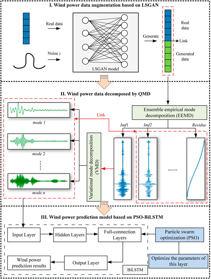
FIGURE 1. The whole process of the LSGAN-QMD-PSO-BiLSTM model.
2.2 Wind power data augmentation based on generative adversarial networks
2.2.1 Generative adversarial network (GAN)
In 2014, Goodfellow et al. (2020) proposed the unsupervised generation model which is called the generative adversarial network (GAN) and is based on game theory. The GAN model involves two deep neural networks: a discriminator (D) and a generator (G). Specifically, the task of the generator is to convert Gaussian noise into the generated data. In each iteration, the new data generated by the generator are evaluated by the discriminator. Then, the generator adapts itself by receiving the information returned by the discriminator. During this game, the generator gradually adapts to the environment (i.e., the discriminator) until the discriminator cannot distinguish the real data from the generated data. Finally, the generator outputs the new data that are similar to the real data. Figure 2 shows the structure of the adversarial networks.

FIGURE 2. The structure of generating adversarial networks.
Mathematically, the rationale of GAN is as follows:
Generator G: In the adversarial process, the input of the generator is a series of Gaussian noise Z sampled from pz, and a series of upsampling operations are performed by the neurons of different functions to output realistic scenarios (Chen et al., 2018). G’s training is performed to capture the real data distribution pr and make the samples generated by it as real as possible. Then, G(z) is taken as the generated sample as well as a new random variable. The loss function of G is expressed as Eq. 1.
Discriminator D: During the game, the discriminator and the generator are trained simultaneously. The input to D consists of real historical data and the data G(z) generated from G. It is expected that D can make correct decisions on the input data. D is aimed at minimizing its loss function, and the parameters of D are updated during adversarial proceedings (Yin et al., 2021). The loss function of D is thus expressed as Eq. 2.
Considering the training objective of the dual-player minimax game, Eqs 1, 2 are combined to establish the complete loss function of the traditional GAN as shown in Eq. 3, where D(x) and D(G(z)) represent the discriminant results of the discriminator on the true input and the generated random variable, respectively.
2.2.2 Least-square generative adversarial network (LSGAN)
The sigmoid cross-entropy loss function is used in the original GANs. When the generator is updated, the loss function widens the gap between the virtual data and the real data edge distribution due to the gradient disappearance encountered by the samples on the real side of the decision boundary. Mao et al. (2017) proposed the least-squares generation antagonism network, which is identical to the original GAN. An a/b mapping strategy intended for the samples is implemented in the discriminator. Herein, a and b represent the labels of generated and real data, respectively.
where c represents the value of the generated data that G attempts to cheat D on.
There are two advantages possessed by LSGAN. On the one hand, LSGAN penalizes the samples even if they are correctly classified, whereas GAN does not, with loss barely caused to the samples located on the correct side of the decision boundary. The decision boundary and parameters of the discriminator are fixed when the generator is updated. Because of the penalty, the generator produces samples in the direction of the decision boundary. On the other hand, the decision boundary must span the distribution of real data to achieve accurate sample distribution learning, otherwise the learning process would be saturated. Therefore, moving the generated samples closer to the decision boundary can make them better conform to the real data distribution. Moreover, punishing the samples distant from the decision boundary can increase the number of gradients produced when updating the generator, which further resolves gradient disappearance and improves the learning stability of LSGAN.
2.2.3 Data set augmentation by LSGAN
To solve the insufficiency of data on newly-built wind farms as support for the training of prediction models, the application of LSGAN is proposed in this research to augment wind power sample data. The given real training set is inputted into the generator, and the pseudoreal data are outputted after the network reaches the specified number of iterations. Then, the real data are concatenated with the generated data. The parameters of LSGAN are set as follows: a) Generator: it is set up in four dense layers, and the neurons in each layer are set as (100,128), (128,128), (128,128), (128,144). The activation function is ReLU, and the learning rate is set to 0.001; b) Discriminator: four dense layers are also set up, and the neurons in each layer are set as (144,128), (128, 128), (128, 128), (128, 1). The activation function is ReLU, and the learning rate is set to 0.001.
However, the augmentation data are not suitable as the input of the prediction model due to its severe non-stationary property. In the next chapter, the proposed quadratic mode decomposition will be introduced to decompose the wind power sequence carried by the augmented data, which reduces the difficulty in training the prediction models.
2.3 Wind power data decomposition based on the quadratic mode decomposition method
The highest frequency intrinsic mode function generated from EEMD, named IMF1, is fuzzy, and it is difficult to analyze the state of real wind power data distribution accurately. To minimize the volatility and uncertainty in wind power data, this research presents a decomposition method including EEMD and VMD, called quadratic mode decomposition (QMD). The rationales of EEMD and VMD are illustrated as follows.
2.3.1 Ensemble empirical mode decomposition (EEMD)
As a method of signal preprocessing analysis, EMD is widely used to process non-stationary and non-linear signals (Ghezaiel et al., 2017). In essence, it is the stepwise decomposition of the variation or trend of different frequencies in the signal, and the final result is a group of eigenmodes of vibration (IMFs), with each decomposed IMF representing the characteristic signals of different frequencies in the original signal. However, modal aliasing may occur in the course of EMD signal processing, which causes the failure in separating modal functions (Huang et al., 2019). The EEMD method introduces Gaussian white noise into the original signal, and the automatic distribution of the signal in the appropriate time scale is achieved after multiple average calculations. This is effective in solving modal aliasing (Liu et al., 2023b). Wind power is susceptible to significant random fluctuations as well as the impact caused by wind direction, wind speed, and other factors. As a result, there is a lot of noise in the wind power series. To reduce noise, the wind power series is divided using the EEMD algorithm, which enables the removal of random fluctuation components from the series and the extraction of main trend components. Below is how the EEMD is used to decompose the wind power series.
After the wind power data are augmented with GAN, the new wind power data
where
Then, the noise-added wind power data
where J refers to the number of IMFs, and
The above two steps are repeated with different Gaussians until the corresponding IMFs are yielded by K iterations.
Finally, the final IMFs are obtained from all IMFs mean values as calculated by K iterations.
where
The new IMF1 value, indicated by
2.3.2 Variational mode decomposition (VMD)
In general, the intrinsic mode functions (IMFs) generated by EEMD are fixed signals. However, the IMF1 signal is of non-systematic and irregular nature (Liu et al., 2014). As the non-linearity of wind power increases, the IMF1 becomes more irregular, which adds to the difficulty in making predictions. According to (Liu et al., 2014), the accuracy of wind power prediction improved slightly when the IMF1 signal is removed. However, there is no theoretical basis for this research. To address the IMF1 issue, a secondary decomposition approach based on VMD is proposed in this research to further decompose the IMF1 component into sub-series.
The VMD algorithm is completely non-recursive and adaptive (Zhang et al., 2023). It builds a variational problem from the signal decomposition problem and solves it to obtain the best answer. In this way, it is ensured that the decomposed sequence is a modal component with a central frequency and a finite bandwidth, which enables the effective separation of the IMFs at each frequency. Also, the M modal components of the preset scale are obtainable (Wang and Li, 2023). Its core step is to construct and solve the variational constraint problem. Below is the process of implementing VMD for wind power newIMF1(t) values from EEMD.
Firstly, the variational constraint problem is constructed as follows:
where ∂t represents the gradient operation,
Then, the problem is solved by constructing the augmented Lagrange expression L through the introduction of the penalty factor α and Lagrange operator λ into the section:
By iterating
where
Finally, it is evaluated whether each decomposition component meets the preset requirements on error accuracy ɛ:
If the inequality is satisfied, the decomposition components currently obtained are outputted; otherwise, revert to Eq. 13 and Eq. 14 to continue the iterative update.
2.4 The PSO-BiLSTM wind power prediction model
The wind power augmenting and decomposing data generated by the GAN and QMD are processed using the proposed PSO-BiLSTM model to predict the wind power data. Usually, the BiLSTM model relies on its optimizer for parameter updating and iterative calculation. However, the built-in optimizer cannot reach the intensity of big data training required for deep learning, and it tends to fall into optimal local solutions when dealing with optimization problems. As a result, the accuracy of prediction is poor (Zhang et al., 2020). To address this issue, the PSO algorithm with an excellent optimization performance is presented in this research and trapping from local optima to apply the optimizer of the full-connection layer of BiLSTM and keep the original optimizer of the other layers, achieving better prediction performance of BiLSTM. The rationales of BiLSTM, PSO, and their implementation are illustrated as follows.
2.4.1 Bidirectional long short-term memory (BiLSTM)
LSTM is suitable for capturing the long-term dependencies in time series as a variant of recurrent neural networks (RNNs) (Mao et al., 2023a). Distinct from traditional RNN, LSTM overcomes slope disappearance and tends to be more predictive. As shown in Figure 3A, this cell is subjected to control by a cell state and three information gates. There are three input variables and two output variables in each LSTM unit, where xt is the current time-step input, ut−1 is the last time-step unit state, ht−1 is the last time-step hidden state, ut is the current time-step unit state, and ht is the current time-step hidden state. The operation of the LSTM unit consists of three phases. The state update of the LSTM cells is performed using Eqs 15–19.
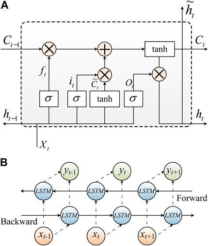
FIGURE 3. (A) The structure of long short-term memory. (B) The structure of Bidirectional Long Short-Term Memory.
where Ft represents the forget gate, It indicates the input gate and Ot denotes the output gate. Sigmoid and tanh are treated as activation functions. In Eqs 16, 17 and 19, ⊗ represents element multiplication. In Eqs 15, 16 and 18, w*x represents the weight parameter of xt, w*h represents the weight parameter of ht−1, and b represents the bias parameter of the three information gates and unit state.
Wind power data show typical time series properties, and the power value at a certain time is related not only to the forward data but also to the reverse data. However, the traditional LSTM is capable to extract data time-related information only in the forward direction. In comparison, the LSTM based on a bidirectional prediction strategy (i.e., BiLSTM) relies on double hidden layers which are opposite in the directions of transmission for connection with the same output layer, which allows the output layer to obtain the information about the past and future states (Cao et al., 2022). Therefore, BiLSTM can extract time-characteristic information in two different directions, thus improving data integrity utilization. The structure of Bidirectional Long-short Time Memory is shown in Figure 3B. The BiLSTM is constructed using a three-layer network with 4, 8 and 16 neurons respectively, and the output layer is a dense one. The activation function is the ReLU function with a drop rate of 0.1 and a learning rate of 0.001.
2.4.2 Particle swarm optimization (PSO)
Proposed by Kennedy and Eberhart (1995), PSO is a random optimization algorithm obtained from the simulation of migration and aggregation of the bird population in its foraging behavior. If a group of birds is foraging at random and there is only one food in this area, the most efficient foraging strategy is to search around the nearest bird for the current prey. The PSO algorithm, which is based on this model, has been widely used to solve various optimization problems. To solve the optimization problem, the potential solution of the problem corresponds to the specific location of a bird in the search space. These “birds” are usually referred to as particles. Each particle keeps flying in space at its own speed and position. In the process of searching for the best position, a group of solutions are generated randomly at first, while the particles in space remember and follow the current best particle to repeat the above process for search in the solution space. With a powerful learning function, PSO can find the next better solution based on the better solution found the previous time. Through cooperation and interaction, it searches for the best local location (pbest) and best global location (gbest) in the search space. The speed and position of all particles are updated as follows:
where X and V represent the current position and speed of the particle, Xnew and Vnew are referred to as the new position and speed of the particle, β indicates the inertia weight to control the impact of historical speed, c1 denotes the cognitive learning factor, c2 stands for the social learning factor, and r1 and r2 represent two independent random numbers in the range of [0,1].
2.4.3 The implementation of PSO in BiLSTM
Despite the significant advantages of the BiLSTM model in the processing of time series data, the full-connection layers (FCL) trained by the popular Adam optimizer perform poorly in the learning rate. Also, it is inclined to fall into the local optima, which affects the prediction performance and the outcome of generalization. Considering the excellent performance of the PSO algorithm in global optimization and convergence speed, PSO is introduced to optimize the FCL parameters of the BiLSTM network, which solves the problems like inaccurate initial connection weight and parameter acquisition for the BiLSTM model. Also, the objectivity of parameter selection is enhanced, and the accuracy of wind power data prediction is improved. Therefore, a combined PSO-BiLSTM model is proposed in this research to predict building carbon emissions in the following steps:
Firstly, a population Z of size P and dimension D is established, where D represents the number of weights and biases of the FCL. It is expressed as Eq. 22.
where hFCL and nout are referred to as the number of network neurons in the front and later layers, respectively.
Then, the weights and biases are randomly generated in population Z to achieve parameter initialization according to the limited rules, including wrange and brange, as shown in Eq. 23.
where b represents the bias of the output layer and θ refers to the offset of the bias.
Each individual in population Z can be expressed as follows:
After the population Z of PSO is established, the fitness of each individual can be calculated by using Eq. 25.
where
The fitness value of the new population as generated by the crossover of PSO is compared with the old one through the greedy mechanism, and the better one stays the particle until the next iteration. In this way, the process is terminated when the maximum number of iterations of the PSO algorithm is reached. Otherwise, the crossover is repeated and the PSO is updated. Finally, the best individual with the optimal fitness value is used to represent the weights and biases of the FCL.
The structure of BiLSTM optimized by PSO is illustrated in Figure 4.
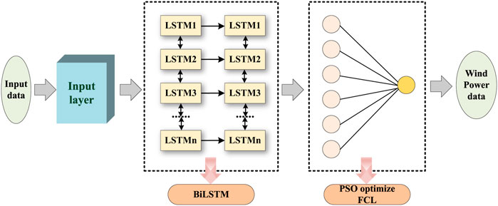
FIGURE 4. The structure of BiLSTM optimized by PSO.
3 Metrics for evaluating the GAN and prediction performance
3.1 The metrics for the GAN model
To assess the performance of this model from different perspectives, five generated data detection tests are performed in this research. Various indicators, including maximum mean deviation (MMD), mean absolute error, root mean square error, cumulative distribution function (CDF), and standard deviation (STD), are used to measure the similarity of distribution between actual data and generated data. The methods of calculation are shown in Eqs 26–30.
3.2 The metrics for prediction performance
To evaluate the wind power prediction performance of the proposed model, three metrics are adopted for this research: root mean square error (RMSE), mean absolute error (MAE), and R-square (R2). Also, RMSE and MAE are used to measure the error between the actual wind power data and the predicted wind power data. R2 is calculated to represent the linear relationship between the input and output data of the prediction model. The calculation results are shown in Eqs 31–33.
where npre represents the number of prediction samples and
4 Case study
In order to evaluate the prediction performance of the proposed LSGAN-QMD-PSO-BiLSTM model, the one-step wind power prediction comparative experiment is performed. All the prediction models are made to run 10 times independently for reduced statistical error. Also, simulation is carried out under the Keras deep learning framework with Python 3.7. Equipped with an Intel Core i5-10210U 1.6 GHz processor and 16 GB memory, the simulation platform runs the Windows 11 operating system.
The wind power data used in this research were sampled from 2/1/2018 to 2/25/2018 at a 10-min interval on the Sotavento-Galicia wind farm in Spain, including a 20-day training data set (2/1/2018 to 2/20/2018) and a five-day test data set (2/21/2018 to 2/25/2018). Figure 5 shows the curves of the data.
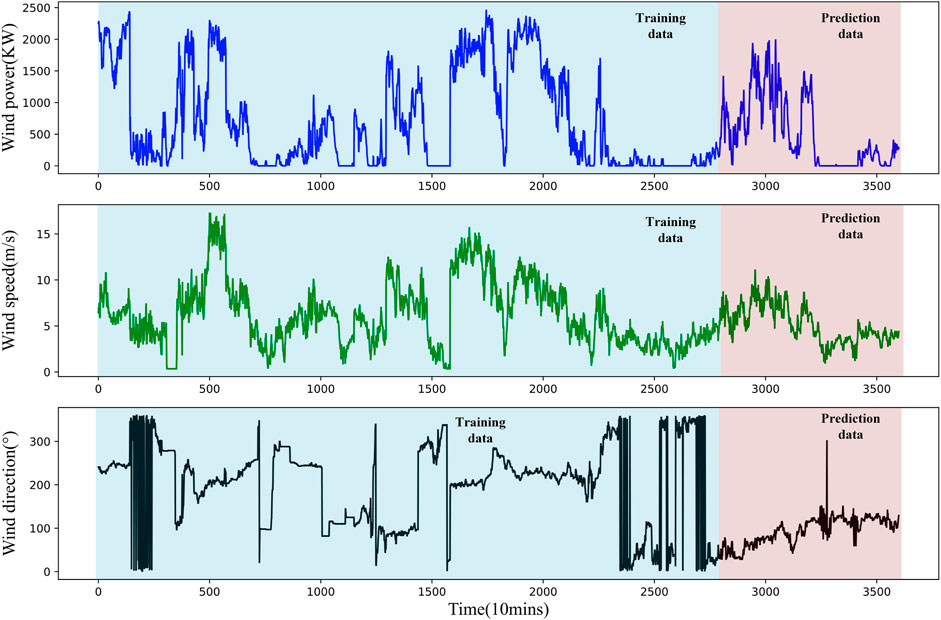
FIGURE 5. The original data of wind power, wind speed, and wind direction.
4.1 Case 1: The effectiveness of PSO-BiLSTM
In this subsection, the PSO-BiLSTM model is verified by conducting two types of experiments. One is to evaluate BiLSTM, and the other is to assess the advantage of applying the PSO algorithm to BiLSTM. Through these experiments, the PSO-BiLSTM model is demonstrated to be effective in predicting wind power for subsequent research on decomposition and data enhancement.
4.1.1 The assessment of BiLSTM
This experiment is intended to identify a single deep-learning model suitable for the combined model proposed in this research to predict wind power. Due to the significant temporal correlation exhibited by the wind power data, four different time series deep learning models represented by RNN are applied in this research, namely, RNN, GRU, LSTM, and BiLSTM. The experiment is carried out using these four models and the benchmark BP model to determine whether the BiLSTM model can outperform the other basic deep learning models in the accuracy of prediction. The errors in wind power prediction are listed in Table 1, and the prediction curves of the wind power are presented inFigure 6A.
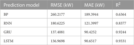
TABLE 1. A comparison between BiLSTM and other basic prediction models.
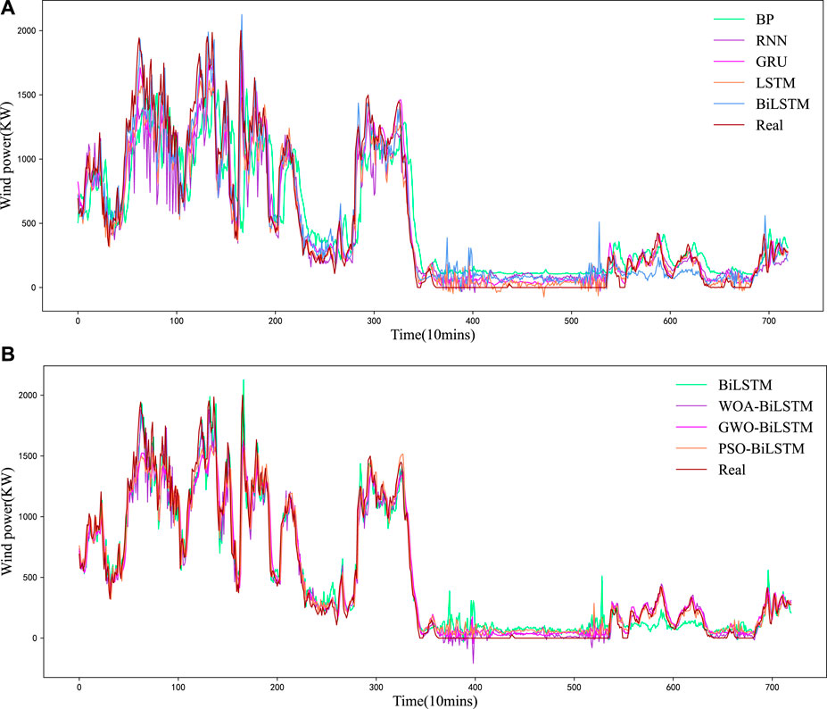
FIGURE 6. (A) The prediction and real wind power curves based on basic forecasting models. (B) The prediction and real wind power curves based on optimized forecasting models.
According to Table 1, the BiLSTM model outperforms the other basic prediction models in the accuracy of prediction. For example, in comparison with the RNN model, the RMSE and MAE errors are reduced by 26.37% and 28.81%, respectively; in comparison with the LSTM model, the RMSE and MAE errors are reduced by 2.91% and 4.68%, respectively. In addition, the prediction wind power curve of BiLSTM is found closer to the real data curve than the prediction curves of other models, as shown in Figure 6A. The BiLSTM model performs best, with the minimum RMSE error, the minimum MAE error, and the optimal R2 value. It is demonstrated that the BiLSTM model is suitable as the original basic wind power prediction model for research.
4.1.2 A comparison between PSO and other optimization algorithms
The proposed PSO-BiLSTM model relies on the PSO algorithm to optimize the FCL weights and bias in BiLSTM. PSO algorithm is characterized by few parameters, fast convergence, and low computational difficulty, for which it has been widely applied to deal with various non-convex, non-linear optimization problems. However, further experimental research is still required to optimize the parameters of deep learning models for wind power prediction with few samples. To solve this problem, the PSO algorithm is applied in this sub-section to optimize the BiLSTM model for experimentation, and a comparison is performed with three different well-known optimization algorithms intended for optimizing BiLSTM, including the whale optimization algorithm (WOA) and gray wolf optimization (GWO) algorithm, and the original model of the ADMM optimizer. Table 2 lists their wind power prediction errors, and Figure 6B presents the predicted wind power curves.
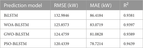
TABLE 2. A comparison between PSO and other optimizers.
As can be seen from Table 2, the PSO-BiLSTM model achieves a better prediction performance than the original BiLSTM model with the ADMM optimizer on RMSE, MAE, and R2 by 9.43%, 8.91%, and 0.62%, respectively. Also, the PSO algorithm outperforms the other two algorithms. Compared with the WOA-BiLSTM and GWO-BiLSTM models, the RMSE, MAE, and R2 of the PSO-BiLSTM model improve by 4.31%, 5.24%, and 0.44%, as well as 3.25%, 2.91%, and 0.53%, respectively.
In addition, Figure 6B shows that the wind power prediction curve of PSO-BiLSTM is closer to the real data curve of other models, especially that of BiLSTM, which suggests the outstanding wind power prediction performance of the PSO-BiLSTM model.
4.2 Case 2: The validity of the QMD method
4.2.1 The effectiveness analysis of QMD based on BiLSTM
In this subsection, the wind power data are decomposed into several time series by the proposed QMD method, including EEMD and VMD. Figure 7 shows the wind power decomposition series. Also, the results obtained by using the EEMD method for wind power IMFs and those obtained by using the VMD method for wind power EEMD IMF-1 are shown in the figures below.
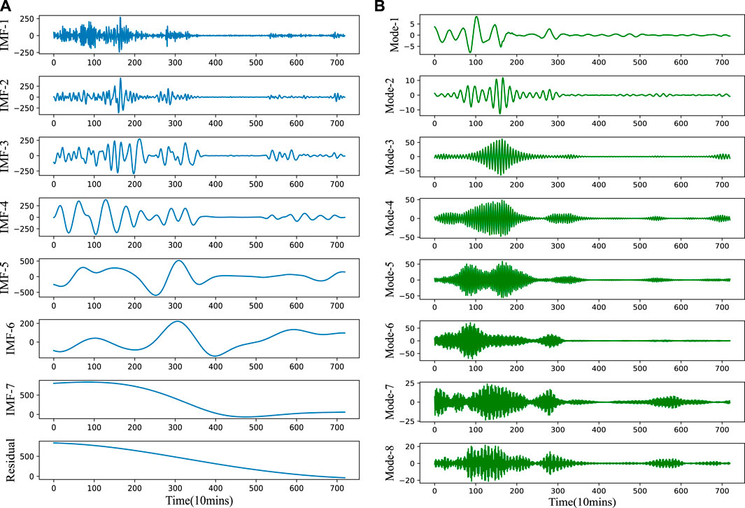
FIGURE 7. The decomposition results of wind power series by the QMD method. (A) EEMD results from original data. (B) VMD results from IMF-1 of EEMD.
Additionally, an experiment is conducted to compare the QMD method based on the secondary decomposition of EEMD and VMD with the EEMD and VMD subjected to decomposition once, as well as the undecomposed prediction method, for verifying the QMD method in terms of improving the accuracy of wind power prediction. It involves the EEMD-BiLSTM, VMD-BiLSTM, QMD-BiLSTM and original BiLSTM models. The errors in wind power prediction are shown in Figure 8A, and the wind power prediction curves are presented in Figure 8B.
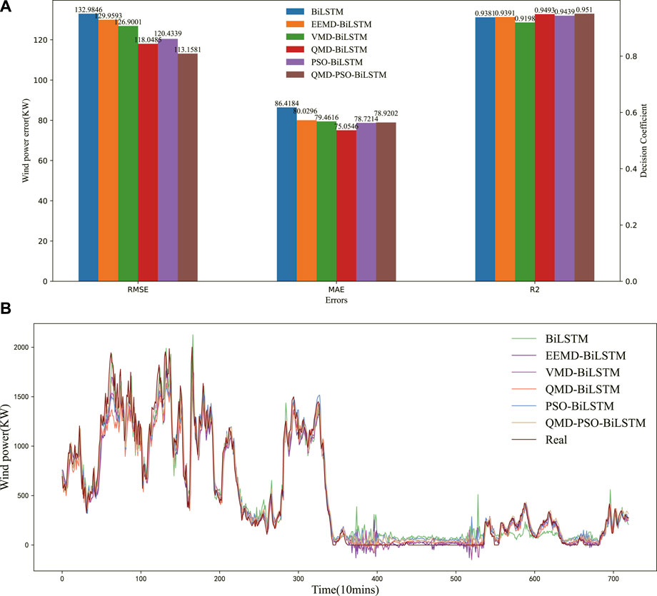
FIGURE 8. (A) The prediction experiment verification of QMD method. (B) The prediction and real wind power curves based on optimized forecasting models.
According to the prediction results, applying the QMD method to decompose the wind power series can improve the accuracy of forecasting relative to the single decomposition method or the original data without decomposition. For example, compared with the EEMD-BiLSTM and VMD-BiLSTM models, the QMD-BiLSTM model outperforms them in all errors by 9.17%, 6.22%, and 1.07%, as well as 6.97%, 5.55%, and 1.01%, respectively. In particular, compared with the original data of the BiLSTM model, the QMD-BiLSTM model reduces the errors significantly by 11.23%, 13.16%, and 1.18%. Furthermore, compared with the other prediction curves shown in Figure 8B, the wind power curve of PSO-BiLSTM is the closest to the real data curve. These results show that the proposed QMD model is capable to improve the prediction performance of BiLSTM.
4.2.2 The verification of QMD-PSO-BiLSTM
In this subsection, the QMD-BiLSTM, PSO-BiLSTM and QMD-PSO-BiLSTM models are experimentally compared to explore the role of the PSO algorithm in the QMD-BiLSTM model. The wind power prediction errors are shown in Figure 8A, and the wind power prediction curves are illustrated in Figure 8B.
According to the prediction results, compared with the PSO-BiLSTM model, the QMD-PSO-BiLSTM model shows a slightly more significant MAE error for its stability, but it still outperforms the PSO-BiLSTM model in RMSE and R2 errors by 6.04% and 0.84%, respectively. Furthermore, compared with the other prediction curves in Figure 8B, the wind power curve of the QMD-PSO-BiLSTM model produces the best-fitting effect with the real data curve. The above analysis shows that the proposed QMD model plays an important role in the PSO-BiLSTM model.
4.3 Case 3: The application of LSGAN-QMD-PSO-BiLSTM in wind power forecasting
4.3.1 Metrics of the samples generated from LSGAN
To evaluate the performance of the proposed LSGAN accurately, it is compared with several typical generative adversarial network models, such as the original GAN, Wasserstein GAN, and deep convolutional generative adversarial network (DCGAN). It is worth noting that the generator and discriminator of all GANs adopt a four-layer convolutional neural network, in which the activation function is ReLU, the convolution kernel is 3, the convolutional step is 2, the number of iterations is 500, and the training batch is 32. To simulate few-shot learning based on the data augmentation method, the samples with a length of 20 days in the original data are treated as the training set of the GAN network. Notably, the input of the generator is the 100-dimensional noise following Gaussian distribution, while the output is the pseudotrue new data. The input of the discriminator is the new data and the original true data, while its output is the discriminant result (that is, true or false). In this section, the evaluation indicators described in Section 3.1 are applied to verify the generation performance of different GAN models in terms of statistical similarity, resemblance, and modal diversity.
4.3.1.1 Modal diversity
The STD method is applied to ascertain whether the generated data are similar to the real data in modal diversity and to track the implied noise in the data. Figure 9A shows the STD curves of wind speed, wind direction, and wind power as drawn by using different GAN models. As shown in Figure 9A, the blue, yellow, and green curves, which respectively represent GAN, WGAN, and DCGAN, fluctuate more often at an interval that is significantly different from the original data. That is to say, the data generated by these three models are different from the original true data in modal diversity, and there is more noise caused. While, the red curve representing LSGAN is more similar to the blue curve that shows the real data within the fluctuation range, and the frequency of fluctuation is comparable to that of the real data. It means that LSGAN is applicable to generate new data with a similar level of modal diversity to the real data but with less noise.

FIGURE 9. STD and CDF of data generated by LSGAN and other augmentation methods. (A) STD values. (B) CDF values.
4.3.1.2 Resemblance
In this research, MMD is adopted to measure the difference between real training data and the data generated by various GAN models. Table 3 shows the minimum MMD of the data generated by LSGAN, indicating that the distribution generated by LSGAN is most similar to the target distribution.

TABLE 3. Scores of various evaluation metrics by GAN, WGAN, DCGAN, and the proposed LSGAN.
4.3.1.3 Statistical similarity
Three indexes are applied to study the statistical similarity of the generated data. Table 3 lists the calculation results of RMSE, MAE, and R2, while Figure 9B shows the CDF visualization of the data of each GAN model. As shown in Figure 9B, the purple curve representing LSGAN and the blue curve of the real data fall within the range of the time series, while GAN and WGAN perform poorly in this aspect. Besides, the performance of LSGAN on RMSE and MAE indexes is superior to other generation models. To sum up, the proposed LSGAN performs better than other GANs in generating statistical similarity to the original data.
4.3.2 The validity of wind power prediction with LSGAN
In this subsection, the proposed LSGAN and GAN models are combined with the basic BiLSTM model to conduct the comparative experiment for verifying both the impact of enhanced data on wind power prediction and the auxiliary prediction effect of the enhanced training set in the proposed LSGAN and GAN models. The unaugmented data are
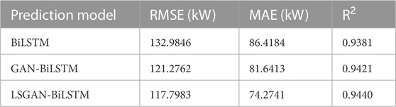
TABLE 4. Results of evaluation indices obtained by using the unaugmented and augmented training data sets.
According to the results shown in Table 4 about RMSE, MAE and R2, using the GAN-enhanced training data set can improve the accuracy of wind forecasting significantly for the newly-built wind farms. The proposed LSGAN-BiLSTM outperforms other non-enhanced or enhanced prediction models in short-term wind power prediction, with a minimum RMSE of 117.7983 (kW), MAE of 74.2741 (kW), and R2 of 0.9440. Also, it achieves an improvement on the BiLSTM model by 11.42%, 14.06%, and 0.63%, respectively, which confirms the advantage of the proposed LSGAN in wind power prediction for newly-built wind farms in the context of data insufficiency.
Furthermore, in order to reveal the impact of the data-augment model on the prediction model under the condition of different data lengths, GAN and LSGAN are applied to enhance the samples of different lengths separately. Also, BiLSTM is used to predict the test set of the following day. R-Square results are obtained, as shown in Table 5.
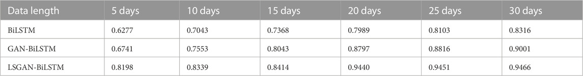
TABLE 5. R2 index results of prediction model under different training set length scenarios.
As can be seen from Table 5, in the absence of data enhancement, the effect of simple BiLSTM prediction is unreliable, especially when the training data span less than 25 days, and R2 indexes are all very low. Meanwhile, when the training data of the LSGAN model span only 5–15 days, the accuracy of prediction remains unsatisfactory. Besides, when the training data span 20 days, the accuracy of prediction reaches 0.9440, which is 15.15%, 13.20%, and 12.19% higher than in the previous three scenarios, respectively. As the span of training data reaches 25 and 30 days, the accuracy of prediction by LSGAN-BiLSTM is also improved, but not to the same extent as the 20-day data. To be exact, the improvement is only 0.116% and 0.275%. That is to say, the proposed LSGAN can assist the prediction model given only 20 days’ worth of data and a limited length of the training set.
4.3.3 Performance of the proposed LSGAN-QMD-PSO-BiLSTM model
To verify the wind power prediction model which is proposed in this research to combine LSGAN, QMD and PSO-BiLSTM, the entire wind power forecasting experiment is performed in this subsection by using the LSGAN-QMD-PSO-BiLSTM, GAN-QMD-PSO-BiLSTM and QMD-PSO-BiLSTM models for comparison with the QMD-BiLSTM and PSO-BiLSTM models. The errors in wind power prediction are shown in Figure 10A, and the curves of wind power forecasting are presented in Figure 10B.
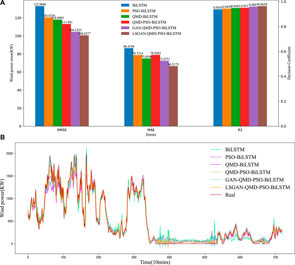
FIGURE 10. (A) Prediction error results among the different decomposition methods; (B) The prediction and real wind power curves among the different decomposition methods.
The proposed LSGAN-QMD-PSO-BiLSTM model outperforms all the comparison models. For example, relative to the GAN-QMD-PSO-BiLSTM and QMD-PSO-BiLSTM models, the proposed model significantly reduces the errors by 3.72%, 8.22%, and 0.33%, as well as by 11.06%, 15.71%, and 1.34%, which evidences the effectiveness of LSGAN in combining the QMD and PSO-BiLSTM methods. Compared with the PSO-BiLSTM and QMD-BiLSTM models, the proposed model reduces the errors by 16.43%, 15.49%, and 2.07%, as well as by 14.74%, 11.37%, and 1.51%. In addition, compared with other prediction curves shown in Figure 10B, the wind power curve of LSGAN-QMD-PSO-BiLSTM is the closest to the real data curve. The above findings confirm the advantage of the wind power prediction model proposed in this research over the persistence model and other decomposition-based or optimization-based hybrid forecasting models in terms of short-term few-sample wind power forecasting.
To objectively evaluate the proposed LSGAN-QMD-PSO-BiLSTM wind power prediction model, the errors are shown as a bar chart in Figure 10A. Apparently, the proposed model achieves the highest accuracy of wind power forecasting in all circumstances, implying that the proposed prediction model performs best consistently.
5 Conclusion
In this research, a wind power prediction method based on LSGAN-QMD-PSO-BilSTM is proposed to address the low accuracy of power prediction caused by a lack of data on newly-built wind farms. The analysis of the actual case allows for the following four deductions.
(1) This research presents a quadratic mode decomposition technology to mitigate the impact of fluctuations on power prediction because of the significant fluctuations and randomness in the original wind power data. The experimental results show that the QMD-BiLSTM model outperforms the EEMD-BiLSTM and VMD-BiLSTM models in all error values by 9.17%, 6.22%, and 1.07%, as well as 6.97%, 5.55%, and 1.01%, respectively. The experimental results demonstrate that the proposed QMD method performs better in denoising data than other decomposition techniques or non-decomposition techniques. Meanwhile, there is a significant improvement in the accuracy prediction by the model.
(2) It is proposed in this research to optimize the parameters of BiLSTM full-connection layer by using the PSO algorithm, which addresses the issue that the neuron parameters trained by the common optimizer are prone to the local optimum. Experimental results show that the PSO-BiLSTM model produces a better prediction performance than the original BiLSTM model with the ADMM optimizer in RMSE, MAE, and R2 by 9.43%, 8.91%, and 0.62%, respectively. According to the experimental results, the proposed PSO-BiLSTM outperforms the unoptimized or other optimization algorithms in preventing the parameters from falling into the local optimum and improving the accuracy of prediction by the model.
(3) Due to the lack of data on newly-built wind farms, LSGAN is first used to determine the edge distribution of actual data before pseudotrue new samples are created to complete data augmentation for the training set. Experimental results show that LSGAN-BiLSTM outperforms other unenhanced or enhanced prediction models (like the BiLSTM model) in short-term wind power prediction by 11.42%, 14.06%, and 0.63%, respectively, with a minimum RMSE of 117.7983 (kW), MAE of 74.2741 (kW), and R2 of 0.9440. The proposed LSGAN outperforms the other algorithms in terms of generating high-quality data and improving the accuracy of power prediction.
(4) The effectiveness of LSGAN in combining the QMD and the PSO-BiLSTM methods is demonstrated by comparing it with the GAN-QMD-PSO-BiLSTM and QMD-PSO-BiLSTM models. It is found that the proposed model reduces the error significantly by 3.72%, 8.22%, and 0.33%, as well as 11.06%, 15.71%, and 1.34%, respectively. The proposed LSGAN-QMD-PSO-BilSTM method achieves the lowest error-index and the highest prediction accuracy when compared to other comparison methods.
Allowing for the excellent performance of this method, more forecasting scenarios will be included in our future research, such as photovoltaic generation forecasting or load forecasting. However, a limitation facing this research is that the simulation is performed using only the data collected from the Sotavento wind farm and only meteorological features are considered. Therefore, the data sets carrying more meteorological characteristics will be analyzed in the future to explore other influencing factors and improve the accuracy of prediction.
Data availability statement
The original contributions presented in the study are included in the article/Supplementary Material, further inquiries can be directed to the corresponding author.
Author contributions
HH: conceptualization, supervision, methodology, software data curation, and writing original draft. MY: investigation, visualization, resources, and formal analysis. All authors contributed to the article and approved the submitted version.
Acknowledgments
We deeply appreciate the invaluable comments from all the reviewers.
Conflict of interest
The authors declare that the research was conducted in the absence of any commercial or financial relationships that could be construed as a potential conflict of interest.
Publisher’s note
All claims expressed in this article are solely those of the authors and do not necessarily represent those of their affiliated organizations, or those of the publisher, the editors and the reviewers. Any product that may be evaluated in this article, or claim that may be made by its manufacturer, is not guaranteed or endorsed by the publisher.
References
Al-Andoli, M. N., Tan, S. C., Sim, K. S., Lim, C. P., and Goh, P. Y. (2022). Parallel deep learning with a hybrid bp-pso framework for feature extraction and malware classification. Appl. Soft Comput.131, 109756. doi:10.1016/j.asoc.2022.109756
Bendaoud, N. M. M., Farah, N., and Ben Ahmed, S. (2021). Comparing generative adversarial networks architectures for electricity demand forecasting. Energy Build.247, 111152. doi:10.1016/j.enbuild.2021.111152
Cai, H., Wu, Z., Huang, C., and Huang, D. (2019). Wind power forecasting based on ensemble empirical mode decomposition with generalized regression neural network based on cross-validated method. J. Electr. Eng. Technol.14, 1823–1829. doi:10.1007/s42835-019-00186-x
Cao, W., Zhou, J., Xu, Q., Zhen, J., and Huang, X. (2022). Short-term forecasting and uncertainty analysis of photovoltaic power based on FCM-WOA-BILSTM model. Front. Energy Res.10, 926774. doi:10.3389/fenrg.2022.926774
Chen, W., Qi, W., Li, Y., Zhang, J., Zhu, F., Xie, D., et al. (2021). Ultra-short-term wind power prediction based on bidirectional gated recurrent unit and transfer learning. Front. Energy Res.827. doi:10.3389/fenrg.2021.808116
Chen, Y., Wang, Y., Kirschen, D., and Zhang, B. (2018). Model-free renewable scenario generation using generative adversarial networks. Ieee Trans. Power Syst.33, 3265–3275. doi:10.1109/TPWRS.2018.2794541
Chen, Y., Yu, S., Islam, S., Lim, C. P., and Muyeen, S. M. (2022a). Decomposition-based wind power forecasting models and their boundary issue: An in-depth review and comprehensive discussion on potential solutions. Energy Rep.8, 8805–8820. doi:10.1016/j.egyr.2022.07.005
Chen, Y., Zhao, H., Zhou, R., Xu, P., Zhang, K., Dai, Y., et al. (2022b). CNN-BiLSTM short-term wind power forecasting method based on feature selection. IEEE J. Radio Freq. Identif.6, 922–927. doi:10.1109/JRFID.2022.3213753
De Giorgi, M. G., Campilongo, S., Ficarella, A., and Congedo, P. M. (2014). Comparison between wind power prediction models based on wavelet decomposition with least-squares support vector machine (LS-SVM) and artificial neural network (ANN). Energies7, 5251–5272. doi:10.3390/en7085251
Ding, Y., Chen, Z., Zhang, H., Wang, X., and Guo, Y. (2022). A short-term wind power prediction model based on ceemd and woa-kelm. Renew. Energy189, 188–198. doi:10.1016/j.renene.2022.02.108
Ewees, A. A., Al-qaness, M. A. A., Abualigah, L., and Elaziz, M. A. (2022). Hbo-lstm: Optimized long short term memory with heap-based optimizer for wind power forecasting. Energy Convers. Manag.268, 116022. doi:10.1016/j.enconman.2022.116022
Ge, X., Qian, J., Fu, Y., Lee, W., and Mi, Y. (2022). Transient stability evaluation criterion of multi-wind farms integrated power system. IEEE Trans. Power Syst.37, 3137–3140. doi:10.1109/TPWRS.2022.3156430
Ghezaiel, W., Ben Slimane, A., and Ben Braiek, E. (2017). Nonlinear multi-scale decomposition by emd for co-channel speaker identification. Multimed. Tools Appl.76, 20973–20988. doi:10.1007/s11042-016-4044-4
Goodfellow, I., Pouget-Abadie, J., Mirza, M., Xu, B., Warde-Farley, D., Ozair, S., et al. (2020). Generative adversarial networks. Commun. Acm63, 139–144. doi:10.1145/3422622
Han, Q., Meng, F., Hu, T., and Chu, F. (2017). Non-parametric hybrid models for wind speed forecasting. Energy Convers. Manag.148, 554–568. doi:10.1016/j.enconman.2017.06.021
Hu, J., Luo, Q., Tang, J., Heng, J., and Deng, Y. (2022). Conformalized temporal convolutional quantile regression networks for wind power interval forecasting. Energy248, 123497. doi:10.1016/j.energy.2022.123497
Huang, Q., and Wang, X. (2022). A forecasting model of wind power based on IPSO–LSTM and classified fusion. Energies15, 5531. doi:10.3390/en15155531
Huang, S., Wang, X., Li, C., and Kang, C. (2019). Data decomposition method combining permutation entropy and spectral substitution with ensemble empirical mode decomposition. Meas. (Lond)139, 438–453. doi:10.1016/j.measurement.2019.01.026
Jin, H., Li, Y., Wang, B., Yang, B., Jin, H., and Cao, Y. (2022). Adaptive forecasting of wind power based on selective ensemble of offline global and online local learning. Energy Convers. Manag.271, 116296. doi:10.1016/j.enconman.2022.116296
Kennedy, J., and Eberhart, R. (1995). Proceedings of icnn’95-international conference on neural networks 4.
Li, Y., Wang, R., Li, Y., Zhang, M., and Long, C. (2023). Wind power forecasting considering data privacy protection: A federated deep reinforcement learning approach. Appl. Energy329, 120291. doi:10.1016/j.apenergy.2022.120291
Liu, H., Jin, K., and Duan, Z. (2019). Air PM2.5 concentration multi-step forecasting using a new hybrid modeling method: Comparing cases for four cities in China. Atmos. Pollut. Res.10, 1588–1600. doi:10.1016/j.apr.2019.05.007
Liu, L., Liu, J., Ye, Y., Liu, H., Chen, K., Li, D., et al. (2023a). Ultra-short-term wind power forecasting based on deep bayesian model with uncertainty. Renew. Energy205, 598–607. doi:10.1016/j.renene.2023.01.038
Liu, Z., Li, M., Zhu, Z., Xiao, L., Nie, C., and Tang, Z. (2023b). Health state identification method of nuclear power main circulating pump based on EEMD and OQGA-SVM. Electronics12, 410. doi:10.3390/electronics12020410
Liu, Z., Sun, W., and Zeng, J. (2014). A new short-term load forecasting method of power system based on EEMD and SS-PSO. Neural Comput. Appl.24, 973–983. doi:10.1007/s00521-012-1323-5
Maatallah, O. A., Achuthan, A., Janoyan, K., and Marzocca, P. (2015). Recursive wind speed forecasting based on hammerstein auto-regressive model. Appl. Energy145, 191–197. doi:10.1016/j.apenergy.2015.02.032
Mao, W., Zhu, H., Wu, H., Lu, Y., and Wang, H. (2023). Forecasting and trading credit default swap indices using a deep learning model integrating Merton and LSTMs. Expert Syst. Appl.213, 119012. doi:10.1016/j.eswa.2022.119012
Mao, X., Li, Q., Xie, H., Lau, R. Y., Wang, Z., and Paul Smolley, S. (2017). “Least squares generative adversarial networks,” in Proceedings of the IEEE International Conference on Computer Vision, 2794–2802.
Qi, M., Gao, H., Wang, L., Xiang, Y., Lv, L., and Liu, J. (2020). Wind power interval forecasting based on adaptive decomposition and probabilistic regularised extreme learning machine. Iet. Renew. Power Gener.14, 3181–3191. doi:10.1049/iet-rpg.2020.0315
Qian, Z., Pei, Y., Zareipour, H., and Chen, N. (2019). A review and discussion of decomposition-based hybrid models for wind energy forecasting applications. Appl. Energy235, 939–953. doi:10.1016/j.apenergy.2018.10.080
Ren, G., Wan, J., Liu, J., Yu, D., and Söder, L. (2018). Analysis of wind power intermittency based on historical wind power data. Energy150, 482–492. doi:10.1016/j.energy.2018.02.142
Safari, N., Chung, C. Y., and Price, G. (2017). Novel multi-step short-term wind power prediction framework based on chaotic time series analysis and singular spectrum analysis. Ieee Trans. Power Syst.33, 590–601. doi:10.1109/TPWRS.2017.2694705
Wang, J., Qin, S., Zhou, Q., and Jiang, H. (2015). Medium-term wind speeds forecasting utilizing hybrid models for three different sites in Xinjiang, China. Renew. Energy76, 91–101. doi:10.1016/j.renene.2014.11.011
Wang, J., Wang, S., and Yang, W. (2019). A novel non-linear combination system for short-term wind speed forecast. Renew. Energy143, 1172–1192. doi:10.1016/j.renene.2019.04.154
Wang, K., Qi, X., Liu, H., and Song, J. (2018). Deep belief network based k-means cluster approach for short-term wind power forecasting. Energy165, 840–852. doi:10.1016/j.energy.2018.09.118
Wang, N., and Li, Z. (2023). Short term power load forecasting based on bes-vmd and cnn-bi-lstm method with error correction. Front. Energy Res.10, 1995. doi:10.3389/fenrg.2022.1076529
Wang, R., Li, C., Fu, W., and Tang, G. (2020). Deep learning method based on gated recurrent unit and variational mode decomposition for short-term wind power interval prediction. IEEE Trans. Neural Netw. Learn. Syst.31, 3814–3827. doi:10.1109/TNNLS.2019.2946414
Wang, Y., Wang, J., and Wei, X. (2015). A hybrid wind speed forecasting model based on phase space reconstruction theory and markov model: A case study of wind farms in northwest China. Renew. Energy91, 556–572. doi:10.1016/j.energy.2015.08.039
Wang, Y., Zou, R., Liu, F., Zhang, L., and Liu, Q. (2021). A review of wind speed and wind power forecasting with deep neural networks. Appl. Energy304, 117766. doi:10.1016/j.apenergy.2021.117766
Xiong, J., Peng, T., Tao, Z., Zhang, C., Song, S., and Nazir, M. S. (2023). A dual-scale deep learning model based on elm-bilstm and improved reptile search algorithm for wind power prediction. Energy266, 126419. doi:10.1016/j.energy.2022.126419
Ye, Y., Strong, M., Lou, Y., Faulkner, C. A., Zuo, W., and Upadhyaya, S. (2022). Evaluating performance of different generative adversarial networks for large-scale building power demand prediction. Energy Build.269, 112247. doi:10.1016/j.enbuild.2022.112247
Yin, H., Ou, Z., Zhu, Z., Xu, X., Fan, J., and Meng, A. (2021). A novel asexual-reproduction evolutionary neural network for wind power prediction based on generative adversarial networks. Energy Convers. Manag.247, 114714. doi:10.1016/j.enconman.2021.114714
Yuan, X., Chen, C., Jiang, M., and Yuan, Y. (2019). Prediction interval of wind power using parameter optimized Beta distribution based LSTM model. Appl. Soft Comput.82, 105550. doi:10.1016/j.asoc.2019.105550
Yunus, K., Thiringer, T., and Chen, P. (2015). ARIMA-based frequency-decomposed modeling of wind speed time series. IEEE Trans. Power Syst.31, 2546–2556. doi:10.1109/TPWRS.2015.2468586
Zhang, G., Tan, F., and Wu, Y. (2020). Ship motion attitude prediction based on an adaptive dynamic particle swarm optimization algorithm and bidirectional lstm neural network. Ieee Access8, 90087–90098. doi:10.1109/ACCESS.2020.2993909
Keywords: short-term wind power prediction, least-square generative adversarial network, quadratic mode decomposition, particle swarm optimization, bidirectional long short-term memory
Citation: He H and Yuan M (2023) A novel few-sample wind power prediction model based on generative adversarial network and quadratic mode decomposition. Front. Energy Res. 11:1211360. doi: 10.3389/fenrg.2023.1211360
Received: 24 April 2023; Accepted: 13 June 2023;
Published: 06 July 2023.
Edited by:
Wen Zhong Shen, Yangzhou University, ChinaReviewed by:
Jingbo Wang, University of Liverpool, United KingdomGuojiang Xiong, Guizhou University, China
Copyright © 2023 He and Yuan. This is an open-access article distributed under the terms of the Creative Commons Attribution License (CC BY). The use, distribution or reproduction in other forums is permitted, provided the original author(s) and the copyright owner(s) are credited and that the original publication in this journal is cited, in accordance with accepted academic practice. No use, distribution or reproduction is permitted which does not comply with these terms.
*Correspondence: Hang He, MjAyMDAxMDg1M0BzdHVkZW50LmN1cC5lZHUuY24=