 Mohammed A. Saeed1
 Abdelhameed Ibrahim2
 El-Sayed M. El-Kenawy3*
 Abdelaziz A. Abdelhamid4,5M. El-Said1,6
 Laith Abualigah7,8,9,10,11Amal H. Alharbi12*
 Doaa Sami Khafaga12
 Osama Elbaksawi13
- 1Electrical Engineering Department, Faculty of Engineering, Mansoura University, Mansoura, Egypt
- 2Computer Engineering Department, College of Engineering and Computer Science, Mustaqbal University, Buraydah, Saudi Arabia
- 3Department of Communications and Electronics, Delta Higher Institute of Engineering and Technology, Mansoura, Egypt
- 4Department of Computer Science, College of Computing and Information Technology, Shaqra University, Shaqra, Saudi Arabia
- 5Department of Computer Science, Faculty of Computer and Information Sciences, Ain Shams University, Cairo, Egypt
- 6Delta Higher Institute of Engineering and Technology, Mansoura, Egypt
- 7Hourani Center for Applied Scientific Research, Al-Ahliyya Amman University, Amman, Jordan
- 8MEU Research Unit, Middle East University, Amman, Jordan
- 9School of Computer Sciences, Universiti Sains Malaysia, Penang, Malaysia
- 10Computer Science Department, Prince Hussein Bin Abdullah Faculty for Information Technology, Al Al-Bayt University, Mafraq, Jordan
- 11Applied Science Research Center, Applied Science Private University, Amman, Jordan
- 12Department of Computer Sciences, College of Computer and Information Sciences, Princess Nourah Bint Abdulrahman University, Riyadh, Saudi Arabia
- 13Electrical Engineering Department, Faculty of Engineering, Port-Said University, Port-Said, Egypt
Wind power forecasting is pivotal in optimizing renewable energy generation and grid stability. This paper presents a groundbreaking optimization algorithm to enhance wind power forecasting through an improved al-Biruni Earth radius (BER) metaheuristic optimization algorithm. The BER algorithm, based on stochastic fractal search (SFS) principles, has been refined and optimized to achieve superior accuracy in wind power prediction. The proposed algorithm is denoted by BERSFS and is used in an ensemble model’s feature selection and optimization to boost prediction accuracy. In the experiments, the first scenario covers the proposed binary BERSFS algorithm’s feature selection capabilities for the dataset under test, while the second scenario demonstrates the algorithm’s regression capabilities. The BERSFS algorithm is investigated and compared to state-of-the-art algorithms of BER, SFS, particle swarm optimization, gray wolf optimizer, and whale optimization algorithm. The proposed optimizing ensemble BERSFS-based model is also compared to the basic models of long short-term memory, bidirectional long short-term memory, gated recurrent unit, and the k-nearest neighbor ensemble model. The statistical investigation utilized Wilcoxon’s rank-sum and analysis of variance tests to investigate the robustness of the created BERSFS-based model. The achieved results and analysis confirm the effectiveness and superiority of the proposed approach in wind power forecasting.
1 Introduction
Growing concerns about the environment and climate change, along with the rapidly increasing capacity of intermittent renewable energy sources, have made forecasting renewable energy generation and, especially, wind energy a vital technology worldwide. The ability to accurately predict power generation from wind farms plays an important role in the world’s transition to a future powered by sustainable energy (Mujeeb et al., 2019; González Sopeña et al., 2023). By the end of the first quarter of 2022, the global installed wind capacity had reached 837 GW, according to the most recent annual report of the Global Wind Energy Council (GWEC) (Global wind report, 2022; Hakami et al., 2022). Wind is an unpredictable and non-constant resource that can experience large swings in performance even over relatively short time periods. Therefore, it is challenging to predict in advance how much wind power can be relied upon at any particular time. Therefore, its potential energy output must be predicted. Accurate wind power forecasting is essential for the smooth incorporation of wind energy into the utilities (Hamid and Alotaibi, 2022a; Cheng et al., 2022; Mahmoud et al., 2022).
There has been a recent uptick in the quest to develop accurate algorithms for forecasting wind power (Ouyang et al., 2019). Physical-based methods, statistical methods, artificial intelligence (AI)-based machine-learning algorithms, and hybrid approaches are the common types (Maldonado-Correa et al., 2020; Hamid and Alotaibi, 2022b). In physical methods, after using atmospheric motion equations to anticipate the development of meteorological readings, physical models would use these estimated readings to make forecasts of wind power (Ding et al., 2018). Several physical methods such as Prediktor, Previento, LocalPred, and eWind use two steps to estimate wind power using numerical weather estimation and physical models. First, wind speed must be anticipated, and then, it must be converted into wind power (Han et al., 2019). However, designing a physical model can be time consuming and expensive, leading to subpar forecast accuracy at the regional scale (Tascikaraoglu and Uzunoglu, 2014).
The data-based statistical models immediately generate functional dependencies from the data to construct a model that describes the links between wind power and other input variables (Bouyeddou et al., 2021), in contrast to the physical techniques based on relatively complex differential equations. Several statistical models, including the autoregressive (AR) model, moving average (MA) model, autoregressive moving average (ARMA) model, and autoregressive integrated moving average (ARIMA) model, provide prediction value as a function of historical wind power (Eissa et al., 2018; Eid et al., 2022). In the work of Rajagopalan and Santoso (2009), the ARMA model was used to predict hourly wind power. Accuracy drops off after 1 hour, but it still does a decent job at predicting the future. These models are straightforward to develop and implement with minimal efforts. It is important to note, however, that while standard time series models (such as ARMA and its derivatives) can achieve a satisfying performance when wind power data show regular changes, the forecast inaccuracy is blatant when the wind power time series shows irregular variations.
One of the recent research-led solutions that generates high-accuracy forecasts for wind farm assets is the use of AI techniques (Couto and Estanqueiro, 2022; Diab and Abdelhamid, 2022). Through advanced analytics, sophisticated instrumentation, and weather data, it helps utility operators increase the integration of wind energy into the grid while improving operational efficiencies, flexibility, and reliability (Cheng et al., 2021; Maray et al., 2022). Hybrid approaches combine several advantages of two or more AI techniques. The AI-based machine-learning techniques and hybrid approaches will be reviewed in Section 1.2.
1.1 Categories of forecasting-based time methods
Based on the needs of the power system, forecasts can be broken down into four distinct time frames: the long term (more than a month ahead), medium term (week, month ahead), short term (day ahead) (Dobschinski et al., 2017), and very short term (few seconds to 30 min ahead) (Soman et al., 2010; Hussah Nasser AlEisa et al., 2022). Figure 1 summarizes the categorization of forecasting methods by time horizon and some of their applications. According to Soman et al. (2010), there are a variety of methods for predicting wind power, each with its own unique set of characteristics and a track record of success in a variety of forecasting environments and time frames.
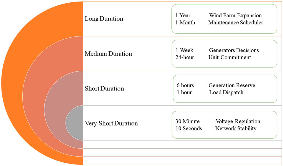
FIGURE 1. Categorization of forecasting methods by time horizon and some of their applications.
1.2 AI-based wind power forecasting techniques
Approaches based on AI have distinct advantages over physical and statistical approaches. AI does not rely on explicit mathematical expressions, and it can learn, organize, and adapt on its own. These techniques utilize historical data and various learning methods to train the network (Jung and Broadwater, 2014). Artificial neural networks (ANNs) and fuzzy logic are commonly used in wind power forecasting. An ANN can model complex relationships and has shown superior results compared to other methods (Jung and Broadwater, 2014; Abdel Samee et al., 2022). Researchers have developed prognostic tools based on ANN modeling to improve system-wide monitoring and management of renewable energy systems (Moustris et al., 2016). Data mining techniques, such as ANN-generated models, have been proven effective for short-term and long-term wind power prediction (Mabel and Fernandez, 2008; Kusiak et al., 2009). Additionally, an ANN can be used to estimate wind speed at a target site based on the correlation with another site (Bechrakis and Sparis, 2004).
Other techniques, such as the Markov method improved by support vector machines (SVMs) and lagged ensemble machine learning, have also been proposed for wind power prediction (Yang et al., 2015; Suárez-Cetrulo et al., 2022). Sparse vector autoregression and mathematical morphology-based local predictors have been employed for short-term probabilistic forecasting (Dowell and Pinson, 2015; Wu et al., 2015). Machine-learning models like random forest regression, support vector regression, k-nearest neighbors, and LASSO regression have been used with daily wind speed data to predict wind power (Demolli et al., 2019; Saber, 2022). Hybrid approaches, combining multiple models, have been effective in increasing prediction accuracy. For example, stacking ensemble learning based on variational mode decomposition and singular spectrum analysis has been used for short-term wind speed forecasting (da Silva et al., 2022). Long short-term memory (LSTM) models trained with heap-based optimizers have shown notable improvements in prediction performance (Ewees et al., 2022). Hybrid approaches using orthogonal tests and SVMs have also demonstrated improved forecasting accuracy (Liu et al., 2017; El-Kenawy et al., 2022a). Additionally, combining the least squares support vector machine with the gravitational search algorithm has resulted in more accurate short-term wind power forecasts (Yuan et al., 2015).
Various machine-learning algorithms, including ANNs, support vector regression, regression trees, and random forest, have been compared for wind power prediction, with support vector regression showing promising results (Buturache and Stancu, 2021; Sami Khafaga et al., 2022). Missing data in wind power prediction have been addressed using multiple imputation techniques based on the expectation maximization algorithm (Liu et al., 2018). Deep-learning frameworks, such as bidirectional gated recurrent units and LSTM, have been employed to automatically model wind speed and power (Xiaoyun et al., 2016; Deng et al., 2019). Adaptive wavelet neural networks have been used to deconstruct wind time series and improve wind power prediction (Bhaskar and Singh, 2012; Shams, 2022). Other methods, such as correntropy LSTM neural networks with improved variational mode decomposition, high-order fuzzy cognitive maps, and Granger causality testing, have been proposed for wind power forecasting (Pei et al., 2022; Qiao et al., 2022; Zhou et al., 2022; Lu et al., 2023). These approaches leverage advanced techniques, optimize models, and extract meaningful features from raw time-series data, resulting in more precise wind power forecasts.
Zhu et al. (2022) presented a hybrid machine-learning technique. First, they used the complete ensemble empirical mode decomposition with an adaptive noise approach to break down the time series into its constituent parts. Second, in order to predict the wind power residuals, a temporal convolutional network-based residual modification model is built, and highly correlated variables are chosen as the model’s input features. The results proved effective in the ability to predict wind power compared to other algorithms.
In the work of Al-qaness et al. (2022), an adaptive neuro-fuzzy inference system (ANFIS) was proposed to deal with wind power forecasting. In order to avoid the algorithm’s early convergence on local optima, the authors developed a new version of the Marine Predator Algorithm (MPA) that makes use of extra mutation operators. They put it to use in fine-tuning the ANFIS’s setup settings. The suggested MPA-ANFIS model was evaluated using information gathered from French wind turbines. They compared their suggested method to previously published algorithms and found that using the MPA-ANFIS improved wind power forecast accuracy. Table 1 summarizes the most important AI-based machine-learning techniques for wind power forecasting.
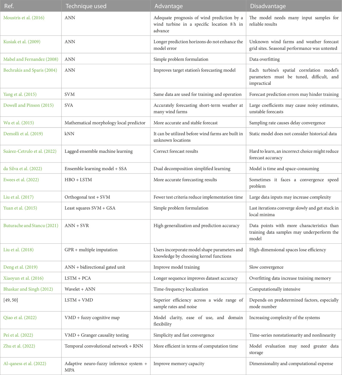
TABLE 1. AI-based machine-learning techniques for wind power forecasting in the literature.
The following is a condensed list of the most important contributions that can be drawn from this body of work:
• Methods based on machine learning are made available for forecasting wind power
• It has been proposed to use an enhanced version of the al-Biruni Earth radius optimization-based stochastic fractal search (BERSFS) algorithm
• A binary BERSFS (bBERSFS) algorithm is proposed for feature selection capabilities from the dataset under test
• In order to improve the accuracy of predictions made using the tested dataset, an optimized ensemble BERSFS-based regression model is being developed
• A comparison of the outcomes produced by various algorithms is carried out in order to identify the one that yields the best results
• The Wilcoxon rank-sum test and the analysis of variance (ANOVA) test are utilized in order to examine whether or not the bBERSFS algorithm and the optimizing ensemble BERSFS-based model have a statistically significant relationship
• The BERSFS-based regression model can be adapted and tested for a variety of datasets because of this method’s flexibility
The remaining parts of this paper are structured as follows. Section 2 provides an overview of the problem statement. Mathematical formulation for wind power forecasting using the al-Biruni Earth radius (BER) model is described in detail in Section 3.Section 4 will discuss some experimental simulations and some cases for comparison. Finally, this paper is concluded in Section 5.
2 Problem statement
If the balance between energy generation and consumption is not kept, there is a risk of disruptions in power quality and supply, which can result in considerable financial loss. The operating security of the power network is dependent on the reliability of the power generation. If wind power predictions are accurate, it will be possible to maximize the contribution of wind energy to the nation’s electrical grid. It was demonstrated that an improvement of approximately 30% in wind power output could be achieved with an increase of 10% in prediction accuracy (Ackermann, 2000). As a result, the development of a wind power prediction model that is very accurate is of utmost importance from a pragmatic standpoint.
The amount of electricity that can be generated by a wind turbine is directly proportional to the average wind speed in the area, which, in turn, is influenced by factors such as the topography of the surrounding area, climate, and changing of the seasons (Soman et al., 2010).
The amount of available and actual wind power that moves across the rotor blades per unit of sweep is defined as
where Pav(v) is the ideal available power, Pactual(v) is the practical wind power, CP is the turbine power conversion coefficient, and ρ(t) is air density in (kg/m3), v is the wind velocity without rotor interference (m/s), and A is the swept area (m2).
The tip angle, the design of the blades, and the relationship between wind speed and rotor speed are the factors that come into play when calculating the Cp for a certain turbine. The maximum power coefficient, often known as the Betz limit, is 0.593 (Bontempo and Manna, 2022). However, it is not possible to obtain this value in actual practice. It was not possible to obtain the power coefficient under a variety of different operating situations. The number 0.5 was utilized for the majority of the practical computations (Bontempo and Manna, 2022). One of the most influential aspects of the wind turbine’s output is the air density. Air density, temperature, and barometric pressure at the location are related according to
where P is the barometric pressure in (Pa), T is the air temperature in (K), R is the specific gas constant for dry air equal to 287.058 (J/(kg.K)), g is the gravity of Earth, 9.81 (m/s2), and h is the hub height above the ground level in (m) (Olaofe, 2014).
3 Materials and methods
3.1 al-Biruni Earth radius algorithm
The original BER optimizes by dividing the population into exploration and exploitation groups. Exploitative and exploratory actions are balanced by changing the agent subgroup makeup. Exploration comprises 70% of the population and exploitation 30%. Increased agent numbers in the exploration and exploitation groups have increased their worldwide average fitness levels. Mathematics helps the exploring team find promising regions nearby. Repeatedly seeking for a fitter option accomplishes this (El-kenawy et al., 2023).
Optimization algorithms discover the best solution given constraints. BER represents population members as S vectors. The vector S = S1, S2, … , Sd ∈ R is the search space size and the optimization parameter or feature d. The fitness function F is recommended for assessing an individual’s performance up to a point. Populations are optimized for a fitness-optimal vector S*. We start with a random population sample (solutions). BER optimizes with the fitness function, lower and higher limits for each solution, dimension, and population size. BER optimization Algorithm 1 is visualized.
This method will be used by the group’s lone explorer to search for promising new areas to investigate in the location they are now in order to get closer to the greatest feasible solution. To achieve this goal, one needs to investigate the many possibilities offered in the neighborhood and select the alternative that is superior to the others concerning the impact on one’s physical wellbeing. The research that BER has carried out makes use of the equations as follows to achieve the equations as follows to achieve this goal:
where the solution vector at iteration t is represented as S(t), and the search agent will search a circle with a diameter of D = r1(S(t) − 1) to look for promising spots. h is an integer that is arbitrarily selected from the range [0, 2], and 0 < x ≤ 180. Examples of coefficient vectors include r1 and r2, and their values can be determined using the equation
The group in charge of making the most of opportunities needs to make the solutions that are already in a better place. . After each round, the BER figures out which participants have reached the highest levels of fitness and awards them accordingly. The BER achieves its goal of exploitation by using two different methods, both of which are explained here. We can get closer to the best solution by using the following equation to move in the right direction.
where r3 is a random vector produced using the equation
Examining the area around the best solution: the most intriguing prospective solution is the area around the best answer (leader). As a result, some people look for methods to improve situations by considering alternatives that are fairly similar to the optimal choice. The process outlined previously is carried out by the BER using the following equation:
where S*(t) represents the best solution. This best solution is selected by comparing S(t+ 1) and S′(t + 1). If the best fitness has not changed during the course of the preceding two iterations, the solution will be altered in accordance with the following equation:
where z represents a random value within [0, 1].
Algorithm 1. BER algorithm
1: Initialize BER population Si(i = 1, 2, … , d) with size d, iterations Tmax, fitness function Fn, t = 1, and parameters of BER
2: Calculate fitness function Fn for each agent Si
3: Find the best solution as S*
4: while t ≤ Tmax do
5: for (i = 1: i < n1 + 1) do
6: Update
7: Move toward the best solution by updating positions as in Eq. 4
8: end for
9: for (i = 1: i < n2 + 1) do
10: Update
11: Elitism of the best solution by updating positions as in Eq. 5
12: Investigating area around the best solution by updating positions as in Eq. 6
13: Select best solution S* by comparing S (t + 1) and S′(t + 1)
14: if the best fitness is the same for the last two iterations, then
15: Mutate solution as in Eq. 7
16: end if
17: end for
18: Update fitness function Fn for each agent Si
19: Find best solution as S*
20: Update parameters of BER and t = t + 1
21: end while
22: Return S*
Algorithm 2. Proposed BERSFS algorithm.
1: Initialize BERSFS population Si(i = 1, 2, … , d) with size d, iterations Tmax, fitness function Fn, t = 1, parameters of BERSFS
2: Calculate the fitness function Fn for each agent Si
3: Find best solution as S*
4: while t ≤ Tmax do
5: if (randBERSFS > 0.5) then
6: for (i = 1: i < n1 + 1) do
7: Update
8: Calculate D = r1(S(t) − 1)
9: Move toward the best solution by updating positions as S (t + 1) = S(t) + D (2r2 − 1)
10: end for
11: for (i = 1: i < n2 + 1) do
12: Update
13: Calculate D = r3 (L(t) − S(t))
14: Elitism of the best solution by updating positions as S (t + 1) = r2(S(t) + D)
15: Calculate
16: Investigating area around the best solution by updating positions as S′(t + 1) = r (S*(t) + k)
17: Select best solution S* by comparing S (t + 1) and S′(t + 1)
18: if the best fitness is the same for the last two iterations, then
19: Mutate solution as
20: end if
21: end for
22: else
23: for (i = 1: i < n + 1) do
24: Calculate updated best solution as S’
25: end for
26: end if
27: Update fitness function Fn for each agent Si
28: Find best solution as S*
29: Update parameters of BERSFS, t = t + 1
30: end while
31: Return S*
The BER chooses the best option for the next cycle to assure quality. Elitism’s efficiency may cause multi-modal functions to converge too soon. The BER can provide excellent exploration capabilities by employing a mutational approach and evaluating all members of the exploration group. Exploration lets the BER delay convergence. Algorithm 1 has the BER pseudo-code. We start by giving the BER population size, mutation rate, and iterations. Then, the BER divides agents into exploratory and exploitative groups. The BER technique automatically adjusts group sizes as it iteratively finds the optimal response. When iterating, the BER will reorder responses to ensure diversity and depth. An exploration group solution may go to the exploitation group in the next iteration. The leader cannot be changed throughout the BER’s exclusive selection process.
3.2 Improved al-Biruni Earth radius algorithm
The time and accuracy of conventional fractals can drive a metaheuristic approach for random fractals. A particle can have electrical potential energy, diffuse, make random particles with the original particle’s energy, and keep the best particles and discard the rest in each generation. The fractal search method uses these three guidelines to solve a problem. Stochastic fractal search (SFS) is a fractal paradigm-based method (El-Kenawy et al., 2020; El-kenawy et al., 2022; Saber and Abotaleb, 2022). SFS can overcome fractal search constraints by using three update mechanisms: diffusion, first, and second. SFS diffusion involves Gaussian walks around the optimal solution (best particle) (El-Kenawy et al., 2022b; Khafaga et al., 2022; Oubelaid et al., 2023).
During the growth process, a random walk is performed using a technique based on the Gaussian distribution. This is performed in order to make it possible for the SFS’s diffusion mechanism to result in the generation of additional particles. During the course of the diffusion process, a list of walks was compiled in accordance with the best possible solution, S*(t). The following is the formula that may be used to calculate the expression:
where the symbol S′*(t + 1) denotes the updated best solution. The η and η′ parameters are made up of random values in the range [0, 1]. The position of the ith point in the group of points surrounding the point is the value denoted by Pi. The values of
The suggested BERSFS algorithm is explained in greater detail in Algorithm 2. The BERSFS algorithm eliminates the negative aspects of the BER and SFS algorithms while maximizing the positive aspects of both in order to generate the response that is best suited for the entire globe. The first thing that has to be carried out in order to complete the technique is to determine the initial positions of d preset agents by utilizing the notation Si(i = 1, 2, … , d). In addition to this, it specifies the parameters for both the BER method and the SFS algorithm, as well as the maximum number of iterations that are permissible throughout the execution process (denoted by Tmax). The term randBERSFS refers to a value that is completely unpredictable and can range from 0 to 1. It lies somewhere in between. If the random variable randBERSFS is greater than 0.5, the BERSFS algorithm will consult the BER equations to figure out how the positions of the agents should be modified. The SFS equations will be employed by the BERSFS algorithm to guide the process of updating the positions of the agents if the random variable for the BERSFS algorithm is less than 0.5.
An expression of the computational complexity presented by the BERSFS method in this research can be seen in the following section. One definition of the complexity is shown in Table 2, which includes iterations Tmax and agents n. According to the preliminary research conducted on the BERSFS method, the level of computational complexity is determined to be O(Tmax × n). This information is presented in this table, where the variable, n, in parentheses refers to the input length and Tmax refers to the max number of iterations.
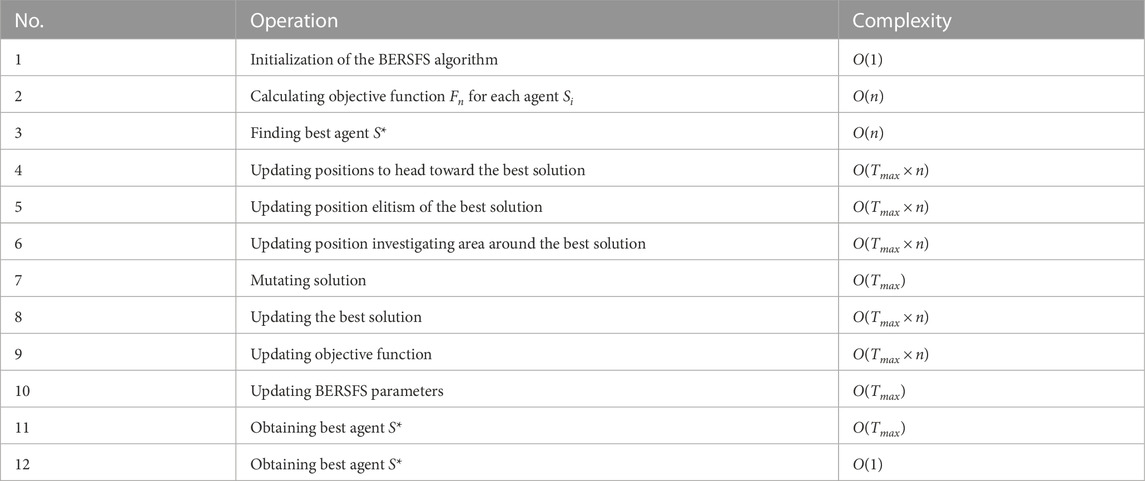
TABLE 2. Computational complexity of the BERSFS algorithm.
4 Experimental results
The findings of this investigation are thoroughly explained in this section. There are two different situations for the experiments. The first scenario covers the proposed bBERSFS algorithm’s feature selection capabilities for the dataset under test, while the second scenario demonstrates the algorithm’s regression capabilities. The BERSFS algorithm is investigated and compared to state-of-the-art algorithms of BER (El-kenawy et al., 2023), SFS (El-Kenawy et al., 2020), particle swarm optimization (PSO) (Bello et al., 2007), gray wolf optimizer (GWO) (El-Kenawy et al., 2020), and whale optimization algorithm (WOA) (Eid et al., 2021). The BERSFS algorithm configuration of all parameters utilized in the experiment is presented in Table 3, while the comparison algorithm setup is presented in Table 4 (Shazly and Khodadadi, 2023).
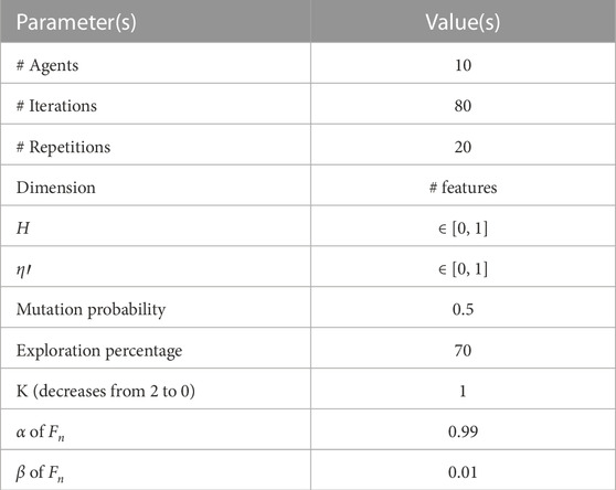
TABLE 3. Configuration parameters of the BERSFS algorithm.
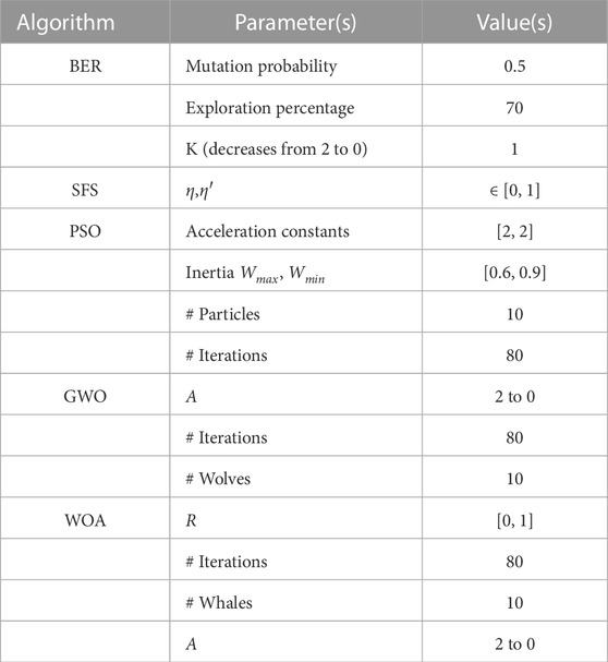
TABLE 4. Compared algorithms’ configuration parameters.
4.1 Dataset
Meteorological data play a crucial role in predicting the wind power output from wind turbines. Various meteorological data are typically included in the data used for short-term wind power prediction in our study.
• Wind speed: It is the most critical meteorological parameter for wind power prediction as it represents the velocity at which the wind is blowing and is typically measured at hub height or at various levels of the turbine. Wind speed data provide valuable information about the available kinetic energy that can be converted into electricity.
• Wind direction: It indicates the compass direction from which the wind is blowing and helps determine the alignment of the wind turbine with respect to the incoming wind. Wind direction is essential in optimizing the turbine’s performance and understanding potential wake effects caused by nearby turbines.
• Ambient temperature: Temperature affects air density, which, in turn, impacts the wind turbine’s power output. Higher temperatures decrease air density, leading to lower power generation. Temperature data are crucial for adjusting the turbine’s performance models accurately.
• Air pressure: It affects wind speed and can indicate weather patterns that might impact wind power generation. It is typically measured at the surface and can be used to infer the presence of high- or low-pressure systems.
• Humidity: Humidity itself might not have a direct impact on wind power prediction but it can indirectly affect atmospheric stability, which influences wind speed and direction.
Renewable sources of energy continue to be one of the most crucial issues to address for a more sustainable future. It is possible that we may fulfill all of our power needs by harnessing the wind, which is a renewable source of energy. Forecasting the power generated by wind farms will be of great assistance as their number continues to grow. The tested data are regarding a specific windmill (Wind power forecasting, 2022). The purpose of using it was to forecast the amount of wind power that could be produced by the windmill over the course of the next 2 weeks. Consequently, a method for the long-term forecasting of wind is required. The dataset includes a variety of aspects related to weather, turbines, and rotors. Data collection began in January 2018 and continued until March of 2020. The readings have been obtained at regular intervals of 10 min. The heatmap that is presented in Figure 2 can be used to gain insight into the manner in which the variables are connected to one another.
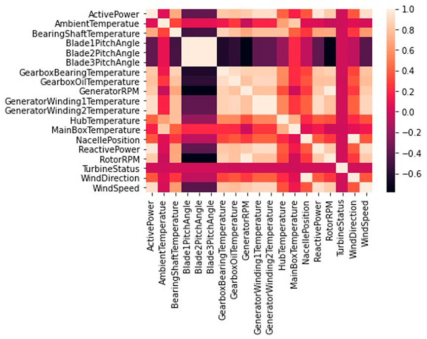
FIGURE 2. Heatmap of the wind power forecasting dataset.
The wind farm installed capacity is 50 MW and consists of 33 single wind turbine units/1,500 kW turbines, each with 1.5 MW nameplate capacity.
• Output data description: The output variable is the active power that could be generated from the wind turbine every 10 min for the next 15 days according to different input variables. It is the power that is available for useful work and is measured in units of W kW (kW).
• Input data description
• Wind speed: Wind speed refers to the rate at which the wind is flowing past a specific point. It is typically measured in units of meters per second (m/s). Wind speed is a fundamental parameter for wind power forecasting as it directly affects the amount of kinetic energy available in the wind, which is essential for estimating the potential power generation of a wind turbine.
• Wind direction: Wind direction refers to the compass direction from which the wind is blowing. It is typically measured in degrees, with 0° indicating a north wind, 90° indicating an east wind, 180° indicating a south wind, and 270° indicating a west wind. Wind direction is a critical parameter for wind power forecasting as it helps determine the alignment of the wind turbine and the efficiency of power generation.
• Ambient temperature: Ambient temperature refers to the temperature of the surrounding environment or air in which a wind turbine operates. It is an important parameter for assessing the performance and efficiency of the turbine and is typically measured in degree Celsius (°C).
• Bearing shaft temperature: Bearing shaft temperature refers to the temperature of the shaft or axle that supports the rotating parts of the wind turbine, such as the rotor or gearbox. Monitoring the bearing shaft temperature is crucial for ensuring the proper lubrication and functioning of the bearings and is typically measured in degree Celsius (°C).
• Blade pitch angle: Blade pitch angle refers to the angle at which the individual blades of a wind turbine are positioned in relation to the oncoming wind. It is a crucial parameter for controlling the power output and aerodynamic performance of the turbine. Each blade can have its own pitch angle, and it is typically measured in degrees.
• Control box temperature: Control box temperature refers to the temperature inside the control or electrical cabinet of a wind turbine. The control box houses various electronic components and systems responsible for controlling and monitoring the turbine’s operation. Monitoring the control box temperature helps ensure the proper functioning and reliability of the electrical systems and is typically measured in degree Celsius (°C).
• Gearbox bearing temperature: Gearbox bearing temperature refers to the temperature of the bearings within the gearbox of a wind turbine. The gearbox is responsible for increasing the rotational speed of the rotor to generate electricity. Monitoring the gearbox bearing temperature is crucial for detecting any potential issues with the lubrication or overheating of the bearings and is typically measured in degree Celsius (°C).
• Gearbox oil temperature: Gearbox oil temperature refers to the temperature of the lubricating oil used in the gearbox of a wind turbine. The gearbox oil plays a critical role in reducing friction and wear between the gears and other moving parts. Monitoring the gearbox oil temperature helps ensure the proper viscosity and functioning of the oil and is typically measured in degree Celsius (°C).
• Generator RPM: Generator RPM (revolutions per minute) refers to the rotational speed at which the generator of a wind turbine is operating. The generator converts the mechanical energy from the rotor into electrical energy. Monitoring the generator RPM helps assess the turbine’s operating speed and is typically measured in RPM.
• Generator winding temperature: Generator winding temperature refers to the temperature of the electrical windings within the generator of a wind turbine. The windings are responsible for producing the electrical output. Monitoring the generator winding temperature is crucial for preventing overheating and ensuring the reliable operation of the generator. The temperature is typically measured in degree Celsius (°C).
• Hub temperature: Hub temperature refers to the temperature at the central hub of the wind turbine, where the rotor blades are attached. Monitoring the hub temperature is important for assessing the thermal conditions and potential heat accumulation in the critical hub area and is typically measured in degree Celsius (°C).
• Main box temperature: Main box temperature refers to the temperature inside the main electrical cabinet or enclosure of a wind turbine. This cabinet houses the main electrical components and systems of the turbine. Monitoring the main box temperature helps ensure the proper functioning and reliability of the electrical systems.
• Nacelle position: The nacelle position refers to the orientation or azimuth angle of the wind turbine nacelle. The nacelle is the housing structure at the top of the wind turbine tower that contains the generator, gearbox, and other components. The nacelle position is typically measured in degrees and is an important parameter for wind power forecasting as it helps determine the direction from which the wind is blowing.
• Rotor RPM: Rotor RPM (revolutions per minute) refers to the rotational speed at which the rotor of a wind turbine is spinning. The rotor is the part of the wind turbine that captures the kinetic energy from the wind and converts it into mechanical energy. Monitoring the rotor revolutions per minute is essential for wind power forecasting as it directly affects the power output of the turbine.
• Turbine status: Turbine status refers to the operational condition of a wind turbine, which can include various states such as running, stopped, faulted, or maintenance mode. Monitoring the turbine status is crucial for wind power forecasting as it helps determine whether the turbine is available and able to generate power or if there are any issues affecting its performance.
4.2 Feature selection scenario
The binary implementation of the BERSFS algorithm that was proposed is what is used to choose features from the dataset that was tested. The first scenario includes a discussion of the results of the feature selection performed by the BERSFS algorithm given in this paper. The binary BERSFS algorithm is investigated and compared to bBER, bSFS, bPSO, bGWO, and bWOA.
In the bBERSFS method, the quality of a solution is evaluated with the help of the objective equation, which is denoted by Fn. Fn is utilized in the equation that is provided in the following section for a classifier’s error rate, Err, a number of selected features, v, and a number of missing features, V.
where beta = 1 − alpha indicates the significance of the supplied feature to the population, and alpha falls in the range [0,1]. If it is possible to give a subset of features that is capable of creating a low classification error rate, then the method can be considered adequate. The kNN technique is an easy classification method that is commonly used. The utilization of the kNN classifier in this method ensures that the characteristics that were selected are of high quality. The shortest distance between the query instance and the training examples is the only factor that is utilized in the process of determining classifiers. No model for the kNN is utilized in this experiment.
The suggested feature selection method’s effectiveness is assessed using the criteria stated in Table 5. The number of runs of the proposed and other competing optimizers is also listed in this table as M. The best solution at run number j is represented by the symbol

TABLE 5. Feature selection evaluation criteria.
Table 6 contains the suggested and contrasted algorithms’ feature selection findings. These results are based on 20 runs and 80 iterations for 10 agents, as detailed in Table 3. The performance of the bBERSFS method that was provided may be seen through the minimum average error of 0.3806 and the standard deviation of 0.0359 with the minimum processing time of 5.623 s. The following best algorithms are bPSO with 0.3908, bBER with 0.3937, bSFS with 0.3991, and then, bWOA with 0.4054, which achieve the lowest minimal average error in the process of feature selection for the data that have been examined. The bGWO algorithm is the worst when it comes to feature selection. It has an error rate of 0.4068 on average. However, the bWOA algorithm is the worst in the processing time of 7.242 s. Table 7 shows the description, including the minimum, median, maximum, and mean average error, of the proposed bBERSFS and other optimization algorithms’ average error results over 12 runs.
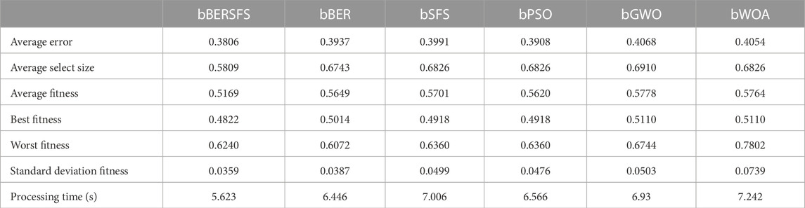
TABLE 6. Proposed bBERSFS versus other optimization algorithms.
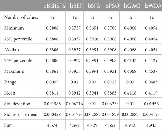
TABLE 7. Description of the proposed bBERSFS and other optimization algorithms’ average error results.
The box plot based on the average error for the proposed bBERSFS algorithm and bBER, bSFS, bPSO, bGWO, and bWOA algorithms is shown in Figure 3. The figure shows the quality of the bBERSFS algorithm using the objective function mentioned in Eq (9). Figure 4 displays the quantile–quantile (QQ) plots, residual plots, and heatmap for both the presented bBERSFS and the methods that were compared for the data that were examined.
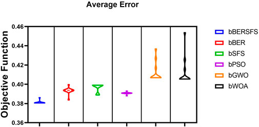
FIGURE 3. Box plot based on the average error for the proposed bBERSFS algorithm and bBER, bSFS, bPSOm bGWO, and bWOA algorithms.
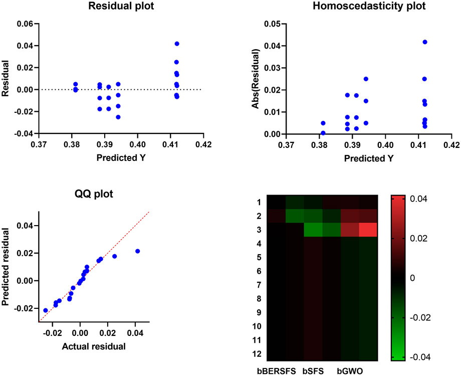
FIGURE 4. Quantile–quantile and residual plots and heatmap for the presented bBERSFS and the methods.
The purpose of this statistical analysis is to establish how well the suggested bBERSFS algorithm performs in terms of the average error by employing a one-way ANOVA and Wilcoxon signed-rank tests. When determining the p-values for a comparison of the suggested method to other algorithms, the Wilcoxon test is the one that is used. With a p-value of less than 0.05, this statistical test can determine whether or not there is a significant difference between the outcomes of the proposed algorithm and those of other algorithms. The ANOVA test was also carried out in order to find out whether or not there is a statistically significant difference between the suggested algorithm and the other algorithms that were examined. The results of the ANOVA test for the proposed algorithm versus the algorithms that were compared are shown in Table 8, and Table 9 also contains a comparison of the proposed algorithm and the algorithms that were compared using the Wilcoxon signed-rank test. In order to ensure that the comparisons are accurate, the statistical analysis is carried out using 12 separate iterations of each of the algorithms that are being presented and evaluated.

TABLE 8. Results of the ANOVA test for the proposed algorithm versus the compared algorithms.
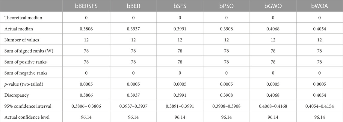
TABLE 9. Comparison of the proposed algorithm and the algorithms that were compared using the Wilcoxon signed-rank test.
4.3 Regression scenario
The experiments’ second scenario discusses the regression results of the proposed optimizing ensemble BERSFS model versus basic models and kNN ensemble model results for 12 runs and 80 iterations using 10 agents as mentioned in Table 4. The basic models are LSTM, bidirectional LSTM (BILSTM), and gated recurrent unit (GRU).
Supplementary measures are utilized in order to assess the effectiveness of the regression models that are utilized in order to forecast wind power. These metrics consist of root-mean-squared error (RMSE), mean absolute error (MAE), mean bias error (MBE), Pearson’s correlation coefficient (r), coefficient of determination (R2), relative root-mean-squared error (RRMSE), Nash–Sutcliffe efficiency (NSE), and determine agreement (WI). With N parameter as the total number of observations in the dataset, the
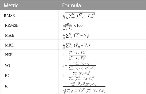
TABLE 10. Prediction evaluation criteria.
Table 11 shows the proposed optimizing ensemble BERSFS-based model versus basic models and kNN ensemble model results. The presented BERSFS-based model achieved an RMSE of 0.00239878, which is the best result compared to the kNN ensemble with an RMSE of 0.007743064. In contrast, LSTM achieved an RMSE of 0.066469754, which is the worst result.
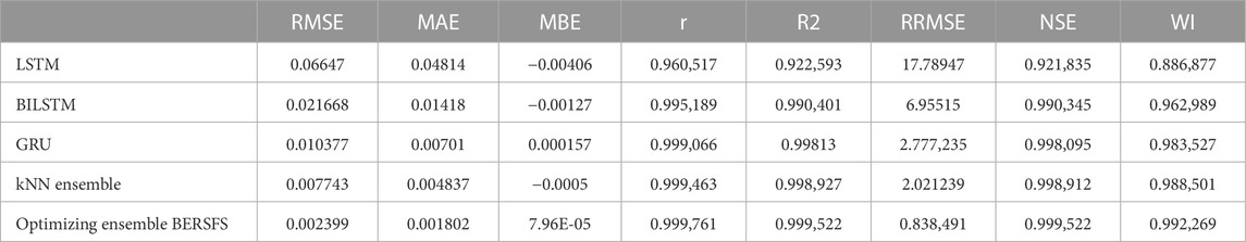
TABLE 11. Proposed optimizing ensemble BERSFS model versus basic models and kNN ensemble model results.
The regression results of the proposed BERSFS-based model are also compared with the BER, SFS, WOA, GWO, and PSO-based models to show the performance of the presented algorithm. Table 12 shows the description, including the minimum, median, maximum, and mean average error, of the proposed BERSFS-based model and other models’ RMSE results over 12 runs.
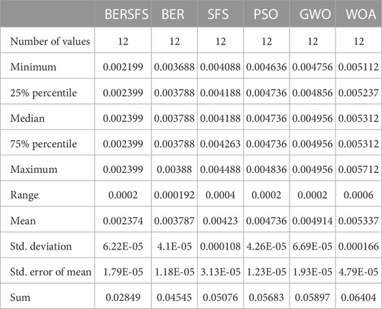
TABLE 12. Description of the proposed BERSFS-based model and other models’ RMSE results.
The box plot based on the RMSE for the proposed BERSFS-based model and BER, SFS, PSO, GWO, and WOA-based models is shown in Figure 5. The figure shows the quality of the optimized ensemble BERSFS-based model using the objective function mentioned in Eq. 9. The histogram of the RMSE for the presented BERSFS-based model and other models is shown in Figure 6. Figure 7 displays the QQ plots, residual plots, and heatmap for both the presented BERSFS-based model and the models that were compared for the data that were examined. These figures show that the presented optimized ensemble BERSFS-based model can perform better than compared models.
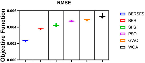
FIGURE 5. Box plot of the proposed BERSFS-based model and BER, SFS, PSO, GWO, and WOA-based models based on the RMSE.
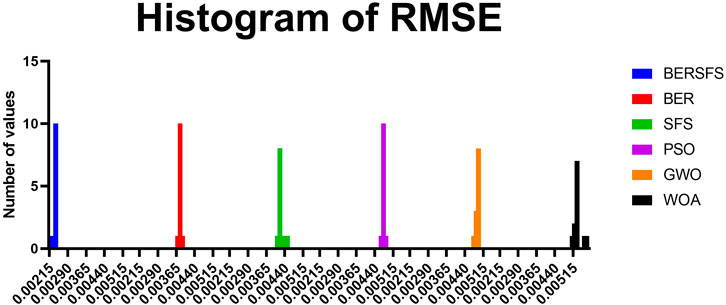
FIGURE 6. Histogram of the RMSE.
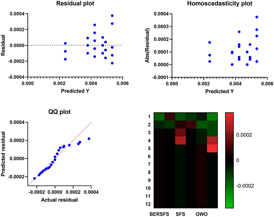
FIGURE 7. QQ plots, residual plots, and heatmap for both the presented BERSFS-based model and the models that were compared.
The results of the ANOVA test for the proposed optimized ensemble BERSFS and the compared models are shown in Table 13, and Table 14 also contains a comparison of the proposed optimized ensemble BERSFS and the compared models using the Wilcoxon signed-rank test. In order to ensure that the comparisons are accurate, the statistical analysis is carried out using 12 separate iterations of each of the algorithms that are being presented and evaluated.

TABLE 13. Results of the ANOVA test for the proposed optimized ensemble BERSFS and the compared models.
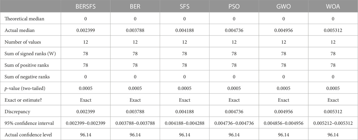
TABLE 14. Comparison of the proposed optimized ensemble BERSFS and the compared models that were compared using the Wilcoxon signed-rank test.
4.4 Time profile
The proposed bBERSFS feature selection algorithm’s convergence time, shown in Figure 8, has been thoroughly compared to that of a number of other feature selection techniques, including bBER, bFSF, bPSO, bGWO, and bWOA. The bBERSFS technique is regularly shown to converge far more quickly than the other approaches in these evaluations. Convergence times for bBER have been demonstrated to be relatively slow. The bFSF approach is also plagued by slow convergence. However, when it comes to feature selection, bPSO, bGWO, and bWOA have all shown to be effective. However, they regularly have slower convergence rates than bBERSFS. Combining the best features of BER and SFS, the bBERSFS algorithm is a hybrid method. Combining the strengths of these two approaches allows bBERSFS to reach optimum feature subsets more quickly. The algorithm’s expanded exploration and exploitation capabilities allow for a more efficient search of the feature space, resulting in a shorter convergence time. The shorter time it takes for bBERSFS to converge is directly translated into substantial time savings while working with feature selection. Researchers and practitioners may save time and energy by receiving their findings more quickly, allowing them to devote their attention where it is most needed. bBERSFS is scalable because of its shortened convergence time, which makes it an excellent choice for feature selection in huge datasets. The suggested bBERSFS algorithm has been shown to achieve faster convergence times than bBER, bFSF, bPSO, bGWO, and bWOA, among other feature selection approaches. These results highlight the promise of bBERSFS as a useful resource in feature selection applications, which will help academics and practitioners save time and effort in their pursuit of optimum feature subsets.

FIGURE 8. Convergence time of the proposed feature selection algorithm.
In addition, the convergence of the proposed optimization algorithm is depicted in Figure 9. In this figure, it can also be noted that the proposed optimization algorithm converges faster than the other optimization methods. These results confirm the superiority of the propose approach in terms of the convergence time.
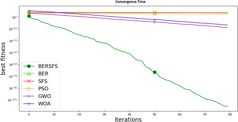
FIGURE 9. Convergence time of the proposed optimization algorithm.
For the adopted dataset, the time (in seconds) consumed in the feature selection and in the optimization process of the model is presented in Table 15. The time taken by each approach in the presented findings is informative about the effectiveness of the suggested methods, particularly bBERSFS for feature selection and BERSFS for optimizing an LSTM, BILSTM, and GRU ensemble model. Convergence for bBERSFS was reported at 85 units in the initial batch of findings. A single unit of time is equivalent to 93 s in bBER, 112 s in bSFS, 117 s in bPSO, 119 s in bGWO, and 125 s in bWOA. These findings show that bBERSFS converges more quickly than the alternative feature selection approaches, which is a significant benefit in terms of efficiency. To further optimize the LSTM + BILSTM + GRU ensemble model, we provide a second set of findings that zeroes in on BERSFS. In this case, we can see that BERSFS has a convergence time of 36.89 units. On the other hand, it takes 41.56 s, 45.36 s, 49.12 s, 51.78 s, and 63.98 s to perform SFS, PSO, GWO, and WOA. By optimizing the ensemble model with much more rapidity, BERSFS once again demonstrates its efficacy. Multiple real-world applications may be drawn from bBERSFS and BERSFS’s dramatic cutting down on convergence time. Researchers and practitioners can speed up the feature selection and ensemble model optimization procedures due to faster convergence. These approaches are more time and effort efficient than their predecessors, allowing for quicker experimentation, analysis, and decision-making. Additionally, bBERSFS and BERSFS’s quicker convergence time helps with their scalability. They excel at solving high-computational expense issues, such as large-scale feature selection and ensemble model optimization. Because of their rapid convergence, these techniques can quickly analyze complicated datasets, which boost the algorithms’ efficiency and performance. Based on the reported convergence times, it is noticeable that the suggested approaches, bBERSFS for feature selection and BERSFS for optimizing the ensemble model, are superior to the alternatives. These findings highlight the benefits of using bBERSFS and BERSFS in practice; academics and practitioners may now speed up convergence and boost productivity in feature selection and ensemble model optimization projects thanks to these findings.

TABLE 15. Time elapsed in feature selection and model optimization (in seconds).
5 Conclusion and future work
The approaches based on AI do not require the use of explicit mathematical expressions, in contrast to the statistical and physical approaches. It can also learn on its own, arrange itself on its own, and adapt to its surroundings without any outside assistance. These techniques make it possible to train the network by using historical data that have already been recorded from each unique location and basing it on a number of learning techniques. The strategies’ foundation in a number of learning techniques makes this possible. A novel component of this research was the use of the updated BER metaheuristic technique, which was based on SFS BERSFS, to increase wind power forecasting accuracy. The proposed approach achieved the following regression results: RMSE = 0.002399, MAE = 0.001802, MBE = 7.96E-05, r = 0.999761, R2 = 0.999522, RRMSE = 0.838491, NSE = 0.999522, and WI = 0.992269. These results proved the effectiveness and accuracy of the proposed method in forecasting the wind power. On the other hand, Wilcoxon’s rank-sum and ANOVA tests were used in the statistical inquiry to examine the robustness of the developed BERSFS-based model. In future work, the BERSFS-based regression model can be adapted and tested for a variety of datasets because of this method’s flexibility and to clearly identify its drawbacks.
Data availability statement
The original contributions presented in the study are included in the article/Supplementary Material; further inquiries can be directed to the corresponding authors.
Author contributions
Conceptualization, EE-K; methodology, MS and EE-K; software, EE-K and AI; validation, OE and ME-S; formal analysis, AA, LA, and DK; investigation, EE-K and AI; writing—original draft, MS and EE-K; writing—review and editing, ME-S, AI, LA, and EE-K; visualization, AA, and DK; and project administration, EE-K. All authors contributed to the article and approved the submitted version.
Funding
This study was supported by Princess Nourah bint Abdulrahman University Researchers Supporting Project number (PNURSP 2023R120), Princess Nourah bint Abdulrahman University, Riyadh, Saudi Arabia.
Conflict of interest
The authors declare that the research was conducted in the absence of any commercial or financial relationships that could be construed as a potential conflict of interest.
Publisher’s note
All claims expressed in this article are solely those of the authors and do not necessarily represent those of their affiliated organizations, or those of the publisher, the editors, and the reviewers. Any product that may be evaluated in this article, or claim that may be made by its manufacturer, is not guaranteed or endorsed by the publisher.
References
Abdel Samee, N., M El-Kenawy, E. S., Atteia, G., Jamjoom, M. M., Ibrahim, A., Abdelhamid, A., et al. (2022). Metaheuristic optimization through deep learning classification of COVID-19 in chest X-ray images. Comput. Mater. Continua 73, 4193–4210. doi:10.32604/cmc.2022.031147
Ackermann, T. (2000). Wind energy technology and current status: A review. Renew. Sustain. Energy Rev. 4, 315–374. doi:10.1016/s1364-0321(00)00004-6
Al-qaness, M. A., Ewees, A. A., Fan, H., Abualigah, L., and Elaziz, M. A. (2022). Boosted ANFIS model using augmented marine predator algorithm with mutation operators for wind power forecasting. Appl. Energy 314, 118851. doi:10.1016/j.apenergy.2022.118851
Bechrakis, D., and Sparis, P. (2004). Correlation of wind speed between neighboring measuring stations. IEEE Trans. Energy Convers. 19, 400–406. doi:10.1109/tec.2004.827040
Bello, R., Gomez, Y., Nowe, A., and Garcia, M. M. (2007). “Two-step particle swarm optimization to solve the feature selection problem,” in Seventh International Conference on Intelligent Systems Design and Applications (ISDA 2007), Brazil, 20-24 October 2007, 691–696. doi:10.1109/ISDA.2007.101
Bhaskar, K., and Singh, S. N. (2012). AWNN-assisted wind power forecasting using feed-forward neural network. IEEE Trans. Sustain. Energy 3, 306–315. doi:10.1109/tste.2011.2182215
Bontempo, R., and Manna, M. (2022). The joukowsky rotor for diffuser augmented wind turbines: Design and analysis. Energy Convers. Manag. 252, 114952. doi:10.1016/j.enconman.2021.114952
Bouyeddou, B., Harrou, F., Saidi, A., and Sun, Y. (2021). “An effective wind power prediction using latent regression models,” in 2021 International Conference on ICT for Smart Society (ICISS), Indonesia, 02-04 August 2021 (IEEE).
Buturache, A. N., and Stancu, S. (2021). Wind energy prediction using machine learning. Low. Carbon Econ. 12, 1–21. doi:10.4236/lce.2021.121001
Cheng, L., Chen, Y., and Liu2PnS-, G. E. G. (2022). 2PnS-EG: A general two-population n-strategy evolutionary game for strategic long-term bidding in a deregulated market under different market clearing mechanisms. Int. J. Electr. Power and Energy Syst. 142, 108182. doi:10.1016/j.ijepes.2022.108182
Cheng, L., Yin, L., Wang, J., Shen, T., Chen, Y., Liu, G., et al. (2021). Behavioral decision-making in power demand-side response management: A multi-population evolutionary game dynamics perspective. Int. J. Electr. Power and Energy Syst. 129, 106743. doi:10.1016/j.ijepes.2020.106743
Couto, A., and Estanqueiro, A. (2022). Enhancing wind power forecast accuracy using the weather research and forecasting numerical model-based features and artificial neuronal networks. Renew. Energy201, 1076–1085. doi:10.1016/j.renene.2022.11.022
da Silva, R. G., Moreno, S. R., Ribeiro, M. H. D. M., Larcher, J. H. K., Mariani, V. C., and dos Santos Coelho, L. (2022). Multi-step short-term wind speed forecasting based on multi-stage decomposition coupled with stacking-ensemble learning approach. Int. J. Electr. Power & Energy Syst. 143, 108504. doi:10.1016/j.ijepes.2022.108504
Demolli, H., Dokuz, A. S., Ecemis, A., and Gokcek, M. (2019). Wind power forecasting based on daily wind speed data using machine learning algorithms. Energy Convers. Manag. 198, 111823. doi:10.1016/j.enconman.2019.111823
Deng, Y., Jia, H., Li, P., Tong, X., Qiu, X., and Li, F. (2019). “A deep learning methodology based on bidirectional gated recurrent unit for wind power prediction,” in 2019 14th IEEE Conference on Industrial Electronics and Applications (ICIEA), China, 19-21 June 2019 (IEEE). doi:10.1109/iciea.2019.8834205
Diab, A. A. Z., and Abdelhamid, A. M. (2022). Optimal identification of model parameters for PEMFCs using neoteric metaheuristic methods. United Kingdom: IET Renewable Power Generation.
Ding, F., Tian, Z., Zhao, F., and Xu, H. (2018). An integrated approach for wind turbine gearbox fatigue life prediction considering instantaneously varying load conditions. Renew. Energy 129, 260–270. doi:10.1016/j.renene.2018.05.074
Dobschinski, J., Bessa, R., Du, P., Geisler, K., Haupt, S. E., Lange, M., et al. (2017). Uncertainty forecasting in a nutshell: Prediction models designed to prevent significant errors. IEEE Power Energy Mag. 15, 40–49. doi:10.1109/mpe.2017.2729100
Dowell, J., and Pinson, P. (2015). Very-short-term probabilistic wind power forecasts by sparse vector autoregression. IEEE Trans. Smart Grid, 1. doi:10.1109/tsg.2015.2424078
Eid, M. M., El-kenawy, E. S. M., and Ibrahim, A. (2021). “A binary sine cosine-modified whale optimization algorithm for feature selection,” in 2021 National Computing Colleges Conference (NCCC) (IEEE), Saudi Arabia, 27-28 March 2021. doi:10.1109/nccc49330.2021.9428794
Eid, M. M., El-Kenawy, E. S. M., Khodadadi, N., Mirjalili, S., Khodadadi, E., Abotaleb, M., et al. (2022). Meta-heuristic optimization of LSTM-based deep network for boosting the prediction of monkeypox cases. Mathematics 10, 3845. doi:10.3390/math10203845
Eissa, M., Yu, J., Wang, S., and Liu, P. (2018). Assessment of wind power prediction using hybrid method and comparison with different models. J. Electr. Eng. Technol. 13, 1089–1098. doi:10.5370/JEET.2018.13.3.1089
El-kenawy, E. S. M., Abdelhamid, A. A., Ibrahim, A., Mirjalili, S., Khodadad, N., duailij, M. A. A., et al. (2023). Al-biruni Earth radius (BER) metaheuristic search optimization algorithm. Comput. Syst. Sci. Eng. 45, 1917–1934. doi:10.32604/csse.2023.032497
El-kenawy, E. S. M., Albalawi, F., Ward, S. A., Ghoneim, S. S. M., Eid, M. M., Abdelhamid, A. A., et al. (2022). Feature selection and classification of transformer faults based on novel meta-heuristic algorithm. Mathematics 10, 3144. doi:10.3390/math10173144
El-Kenawy, E. S. M., Eid, M. M., Saber, M., Ibrahim, A., and MbGWO-, S. F. S. (2020). MbGWO-SFS: Modified binary Grey Wolf optimizer based on stochastic fractal search for feature selection. IEEE Access 8, 107635–107649. doi:10.1109/access.2020.3001151
El-Kenawy, E. S. M., Mirjalili, S., Abdelhamid, A. A., Ibrahim, A., Khodadadi, N., and Eid, M. M. (2022a). Meta-heuristic optimization and keystroke dynamics for authentication of smartphone users. Mathematics 10, 2912. doi:10.3390/math10162912
El-Kenawy, E. S. M., Mirjalili, S., Alassery, F., Zhang, Y. D., Eid, M. M., El-Mashad, S. Y., et al. (2022b). Novel meta-heuristic algorithm for feature selection, unconstrained functions and engineering problems. IEEE Access 10, 40536–40555. doi:10.1109/access.2022.3166901
Ewees, A. A., Al-qaness, M. A., Abualigah, L., and Elaziz, M. A. (2022). HBO-LSTM: Optimized long short term memory with heap-based optimizer for wind power forecasting. Energy Convers. Manag. 268, 116022. doi:10.1016/j.enconman.2022.116022
Global wind report (2022). Global wind report 2022. https://gwec.net/global-wind-report-2022/ (Accessed June 05).
González Sopeña, J. M., Pakrashi, V., and Ghosh, B. (2023). A benchmarking framework for performance evaluation of statistical wind power forecasting models. Sustain. Energy Technol. Assessments 57, 103246. doi:10.1016/j.seta.2023.103246
Hakami, A. M., Hasan, K. N., Alzubaidi, M., and Datta, M. (2022). A review of uncertainty modelling techniques for probabilistic stability analysis of renewable-rich power systems. Energies 16, 112. doi:10.3390/en16010112
Hamid, A., and Alotaibi, S. (2022a). Optimized two-level ensemble model for predicting the parameters of metamaterial antenna. Comput. Mater. Continua 73, 917–933. doi:10.32604/cmc.2022.027653
Hamid, A., and Alotaibi, S. (2022b). Robust prediction of the bandwidth of metamaterial antenna using deep learning. Comput. Mater. Continua 72, 2305–2321. doi:10.32604/cmc.2022.025739
Han, S., hui Qiao, Y., Yan, J., qian Liu, Y., Li, L., and Wang, Z. (2019). Mid-to-long term wind and photovoltaic power generation prediction based on copula function and long short term memory network. Appl. Energy 239, 181–191. doi:10.1016/j.apenergy.2019.01.193
Hussah Nasser AlEisa, A., El-Sayed, M., Ali Alhussan, A., Saber, M., A. Abdelhamid, A., and Sami Khafaga, D. (2022). Transfer learning for chest X-rays diagnosis using dipper Throated algorithm. Comput. Mater. Continua 73, 2371–2387. doi:10.32604/cmc.2022.030447
Jung, J., and Broadwater, R. P. (2014). Current status and future advances for wind speed and power forecasting. Renew. Sustain. Energy Rev. 31, 762–777. doi:10.1016/j.rser.2013.12.054
Khafaga, D. S., Alhussan, A. A., El-Kenawy, E. S. M., Ibrahim, A., Eid, M. M., and Abdelhamid, A. A. (2022). Solving optimization problems of metamaterial and double t-shape antennas using advanced meta-heuristics algorithms. IEEE Access 10, 74449–74471. doi:10.1109/access.2022.3190508
Kusiak, A., Zheng, H., and Song, Z. (2009). Wind farm power prediction: A data-mining approach. Wind Energy 12, 275–293. doi:10.1002/we.295
Liu, T., Wei, H., and Zhang, K. (2018). Wind power prediction with missing data using Gaussian process regression and multiple imputation. Appl. Soft Comput. 71, 905–916. doi:10.1016/j.asoc.2018.07.027
Liu, Y., Sun, Y., Infield, D., Zhao, Y., Han, S., and Yan, J. (2017). A hybrid forecasting method for wind power ramp based on orthogonal test and support vector machine (OT-SVM). IEEE Trans. Sustain. Energy 8, 451–457. doi:10.1109/tste.2016.2604852
Lu, W., Duan, J., Wang, P., Ma, W., and Fang, S. (2023). Short-term wind power forecasting using the hybrid model of improved variational mode decomposition and maximum mixture correntropy long short-term memory neural network. Int. J. Electr. Power & Energy Syst. 144, 108552. doi:10.1016/j.ijepes.2022.108552
Mabel, M. C., and Fernandez, E. (2008). Analysis of wind power generation and prediction using ANN: A case study. Renew. Energy 33, 986–992. doi:10.1016/j.renene.2007.06.013
Mahmoud, F. S., Abdelhamid, A. M., Sumaiti, A. A., El-Sayed, A. H. M., and Diab, A. A. Z. (2022). Sizing and design of a PV-wind-fuel cell storage system integrated into a grid considering the uncertainty of load demand using the marine predators algorithm. Mathematics 10, 3708. doi:10.3390/math10193708
Maldonado-Correa, J., Valdiviezo, M., Solano, J., Rojas, M., and Samaniego-Ojeda, C. (2020). Wind energy forecasting with artificial intelligence techniques: A review. Commun. Comput. Inf. Sci., 348–362. Springer International Publishing). doi:10.1007/978-3-030-42520-3_28
Maray, M., Alghamdi, M., Alrayes, F. S., Alotaibi, S. S., Alazwari, S., Alabdan, R., et al. (2022). Intelligent metaheuristics with optimal machine learning approach for malware detection on iot-enabled maritime transportation systems. Expert Syst. 39. doi:10.1111/exsy.13155
Moustris, K., Zafirakis, D., Kavvadias, K., and Kaldellis, J. (2016). Mediterranean conference on power generation, transmission, distribution and energy conversion (MedPower 2016). Belgrade: Institution of Engineering and Technology. Wind power forecasting using historical data and artificial neural networks modeling. doi:10.1049/cp.2016.1094
Mujeeb, S., Alghamdi, T. A., Ullah, S., Fatima, A., Javaid, N., and Saba, T. (2019). Exploiting deep learning for wind power forecasting based on big data analytics. Appl. Sci. 9, 4417. doi:10.3390/app9204417
Olaofe, Z. O. (2014). A 5-day wind speed & power forecasts using a layer recurrent neural network (LRNN). Sustain. Energy Technol. Assessments 6, 1–24. doi:10.1016/j.seta.2013.12.001
Oubelaid, A., Shams, M. Y., and Abotaleb, M. (2023). Energy efficiency modeling using whale optimization algorithm and ensemble model. J. Artif. Intell. Metaheuristics 2, 27–35. doi:10.54216/JAIM.020103
Ouyang, T., Zha, X., Qin, L., He, Y., and Tang, Z. (2019). Prediction of wind power ramp events based on residual correction. Renew. Energy 136, 781–792. doi:10.1016/j.renene.2019.01.049
Pei, M., Ye, L., Li, Y., Luo, Y., Song, X., Yu, Y., et al. (2022). Short-term regional wind power forecasting based on spatial–temporal correlation and dynamic clustering model. Energy Rep. 8, 10786–10802. doi:10.1016/j.egyr.2022.08.204
Qiao, B., Liu, J., Wu, P., and Teng, Y. (2022). Wind power forecasting based on variational mode decomposition and high-order fuzzy cognitive maps. Appl. Soft Comput. 129, 109586. doi:10.1016/j.asoc.2022.109586
Rajagopalan, S., and Santoso, S. (2009). “Wind power forecasting and error analysis using the autoregressive moving average modeling,” in 2009 IEEE Power & Energy Society General Meeting (IEEE), Canada, 26-30 July 2009. doi:10.1109/pes.2009.5276019
Saber, M., and Abotaleb, M. (2022). Arrhythmia modern classification techniques: A review. J. Artif. Intell. Metaheuristics 1, 42–53. doi:10.54216/JAIM.010205
Saber, M. (2022). Removing powerline interference from EEG signal using optimized FIR filters. J. Artif. Intell. Metaheuristics 1, 08–19. doi:10.54216/JAIM.010101
Sami Khafaga, D., Ali Alhussan, A., M. El-kenawy, E.-S., E. Takieldeen, A., M. Hassan, T., A. Hegazy, E., et al. (2022). Meta-heuristics for feature selection and classification in diagnostic Breast cancer. Comput. Mater. Continua 73, 749–765. doi:10.32604/cmc.2022.029605
Shams, M. Y. (2022). Hybrid neural networks in generic biometric system: A survey. J. Artif. Intell. Metaheuristics 1, 20–26. doi:10.54216/JAIM.010102
Shazly, K., and Khodadadi, N. (2023). Credit card clients classification using hybrid guided wheel with particle swarm optimized for voting ensemble. J. Artif. Intell. Metaheuristics 2, 46–54. doi:10.54216/JAIM.020105
Soman, S. S., Zareipour, H., Malik, O., and Mandal, P. (2010). “A review of wind power and wind speed forecasting methods with different time horizons,” in North American Power Symposium 2010, Arlington, 26-28 September 2010 (IEEE). doi:10.1109/naps.2010.5619586
Suárez-Cetrulo, A. L., Burnham-King, L., Haughton, D., and Carbajo, R. S. (2022). Wind power forecasting using ensemble learning for day-ahead energy trading. Renew. Energy 191, 685–698. doi:10.1016/j.renene.2022.04.032
Tascikaraoglu, A., and Uzunoglu, M. (2014). A review of combined approaches for prediction of short-term wind speed and power. Renew. Sustain. Energy Rev. 34, 243–254. doi:10.1016/j.rser.2014.03.033
Wind power forecasting (2022). Wind power forecasting. https://www.kaggle.com/datasets/theforcecoder/wind-power-forecasting (Accessed December 24, 2022).
Wu, J. L., Ji, T. Y., Li, M. S., Wu, P. Z., and Wu, Q. H. (2015). Multistep wind power forecast using mean trend detector and mathematical morphology-based local predictor. IEEE Trans. Sustain. Energy 6, 1216–1223. doi:10.1109/tste.2015.2424856
Xiaoyun, Q., Xiaoning, K., Chao, Z., Shuai, J., and Xiuda, M. (2016). “Short-term prediction of wind power based on deep long short-term memory,” in 2016 IEEE PES Asia-Pacific Power and Energy Engineering Conference (APPEEC), Xi'an, 25-28 October 2016 (IEEE). doi:10.1109/appeec.2016.7779672
Yang, L., He, M., Zhang, J., and Vittal, V. (2015). Support-vector-machine-enhanced markov model for short-term wind power forecast. IEEE Trans. Sustain. Energy 6, 791–799. doi:10.1109/tste.2015.2406814
Yuan, X., Chen, C., Yuan, Y., Huang, Y., and Tan, Q. (2015). Short-term wind power prediction based on LSSVM–GSA model. Energy Convers. Manag. 101, 393–401. doi:10.1016/j.enconman.2015.05.065
Zhou, X., Liu, C., Luo, Y., Wu, B., Dong, N., Xiao, T., et al. (2022). Wind power forecast based on variational mode decomposition and long short term memory attention network. Energy Rep. 8, 922–931. doi:10.1016/j.egyr.2022.08.159
Zhu, J., Su, L., and Li, Y. (2022). Wind power forecasting based on new hybrid model with TCN residual modification. Energy AI 10, 100199. doi:10.1016/j.egyai.2022.100199
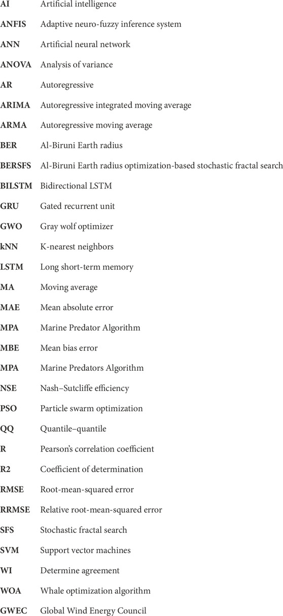
Glossary
Keywords: forecasting wind power, al-Biruni Earth radius, metaheuristic algorithm, artificial intelligence, optimization
Citation: Saeed MA, Ibrahim A, El-Kenawy E-SM, Abdelhamid AA, El-Said M, Abualigah L, Alharbi AH, Khafaga DS and Elbaksawi O (2023) Forecasting wind power based on an improved al-Biruni Earth radius metaheuristic optimization algorithm. Front. Energy Res. 11:1220085. doi: 10.3389/fenrg.2023.1220085
Received: 10 May 2023; Accepted: 15 June 2023;
Published: 13 July 2023.
Edited by:
Wen Zhong Shen, Yangzhou University, ChinaReviewed by:
Mao Yang, Northeast Electric Power University, ChinaLefeng Cheng, Guangzhou University, China
Copyright © 2023 Saeed, Ibrahim, El-Kenawy, Abdelhamid, El-Said, Abualigah, Alharbi, Khafaga and Elbaksawi. This is an open-access article distributed under the terms of the Creative Commons Attribution License (CC BY). The use, distribution or reproduction in other forums is permitted, provided the original author(s) and the copyright owner(s) are credited and that the original publication in this journal is cited, in accordance with accepted academic practice. No use, distribution or reproduction is permitted which does not comply with these terms.
*Correspondence: El-Sayed M. El-kenawy, c2tlbmF3eUBpZWVlLm9yZw==; Amal H. Alharbi, YWhhbGhhcmJpQHBudS5lZHUuc2E=