Economic impact and risk analysis of integrating sustainable aviation fuels into refineries

1 Introduction

The technical, economic, and environmental challenges of integrating sustainable aviation fuels (SAFs) have become a top priority for the renewable fuels industry. Greenhouse gas (GHG) emissions contributed by the aviation industry have grown steadily at a rate of 2.0% per year from 2000 to 2019 to a 2.8% global share of fossil fuel sourced emissions in 2019 (Aviation, 2022). Most concerns, however, stem from the industry consensus that rapid growth will continue over the next 20 years. As of 2019, the International Civil Aviation Organization (ICAO) and Airbus estimate an annual growth rate of 4.3%, while Boeing’s estimate for commercial air transportation demand stood at 4.6% (Future of Aviation, 2019; Global Market Forecast, 2019-2038, 2019; Commercial Market Outlook, 2019-2038, 2019). However, the 66% reduction in global air travel observed in 2020 caused by the COVID-19 pandemic and resulting market changes (teleworking, increasing cargo demand, etc.) exemplified the air transportation industry’s exposure to market risks (Commercial Aerospace Insight Report, 2021). Nonetheless, the transience of events like COVID-19, persistence of long-term drivers for aviation industry growth, and global decarbonization goals combine to make a case for proactively addressing the sector’s climate change potential (Gössling and Humpe, 2020).

The prospect of the aviation industry negating nationally determined contributions (NDCs) submitted by countries under the Paris Climate Agreement (Paris Agreement, 2015) has already prompted action from several international organizations. Perhaps the most widely recognized countermeasures are being taken by the International Civil Aviation Organization (ICAO) with their Carbon Offsetting and Reduction Scheme for International Aviation (CORSIA). CORSIA initiatives aim to achieve carbon neutral growth after 2020 through a combination of operational improvements, decarbonizing propulsion, and purchasing carbon offsets (Climate Change Mitigation: CORSIA, 2019).

ICAO and others acknowledge radical technology shifts like electrification, fuel cells, or hybrid power that are promising for other transportation sectors as potential decarbonization strategies for aviation (Climate Change Mitigation: CORSIA, 2019; Driessen and Hak, 2021). However, the uniquely high energy density requirements of aircraft will likely relegate these strategies to long-term deployment timelines incompatible with CORSIA (Schwab et al., 2021). ICAO currently anticipates over 50% of their decarbonization goals will need to come from SAFs (Climate Change Mitigation: CORSIA, 2019). Moreover, national commitments such as the United State’s SAF Grand Challenge (SAF Grand Challenge Roadmap, 2022) and European Union’s ReFuelEU Aviation Initiative (Soone, 2022), which both set increasingly large SAF blending targets over time, underscore the role of SAF production as the leading strategy to decarbonize aviation.

However, with current global SAF production capacity estimated to be around 800 million gallons per year, amounting to less than 1% of total jet fuel demand, the SAF industry is clearly in its nascent stage (Newsom et al., 2023). Several barriers to adoption have been identified that have previously, and will continue, to challenge SAF market adoption. Primarily, limited feedstock availability, high collection costs, low yields, and immature process technologies have led to uncompetitive SAF prices (Chiaramonti, 2019). Additionally, when biomass resources are available, biorefineries are typically incentivized to produce sustainable diesel with additional tax credits over SAF (Rep Yarmuth, 2022). These challenges, as well as others, make attracting the capital needed to achieve economies of scale, reducing costs, and competing within the petroleum jet market difficult (Shahriar and Khanal, 2022).

Conversely, petroleum refineries, currently producing essentially all jet fuel globally, will be affected by the SAF market’s growth if some of its challenges are successfully addressed. The uncertain landscape in which refineries are currently planning and operating is further complicated by the decarbonization trajectories of the light/heavy duty and marine transportation sectors. The Energy Information Administration’s (EIA) Annual Energy Outlook (AEO) factors long-term market forces such as population growth, consumer behavioral shifts, and technology changes to project transportation fuel demands in the United States to 2050 as displayed in Figure 1 (Annual Energy Outlook, 2022, 2022). An alternative gasoline demand projection from the National Renewable Energy Laboratory’s (NREL) Automotive Deployment Options Projection Tool (ADOPT) that predicts a higher degree of vehicle electrification is also shown (Brooker et al., 2015). Combining these projections elucidates the broader industry’s expectation of gasoline demand either stabilizing or plummeting, with high degrees of uncertainty, alongside steady decreases in diesel and increases in jet fuel demands. These market shifts could set the stage for coordination between petroleum refiners and SAF producers to simultaneously meet increasing volumetric and decarbonization demands for aviation fuels (Global downstream outlook to 2035, 2019).

FIGURE 1

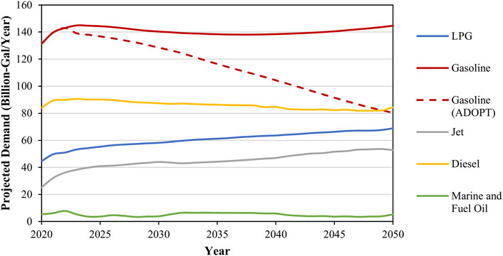
FIGURE 1. EIA’s refinery product demand projections for 6 major product groupings [LPG (C_3-4), Gasoline (C_4-12), Jet (C_8-16), Diesel (C_12-20), Marine and Fuel Oil (C₂₀₊)] in the US alongside the gasoline demand projected by NREL’s ADOPT model (Brooker et al., 2015; ‘Annual Energy Outlook 2022’, 2022).

Numerous conversion pathways are being researched for drop-in SAF production such as alcohol-to-jet, oil-to-jet via hydroprocessing, and Fischer-Tropsch based gas-to-jet, yet no clear winner has emerged (Wang et al., 2016; Boyd, 2022). Supplementally, several refinery integration strategies including direct blending, co-location, co-processing bio-intermediates like pyrolysis or hydrothermal liquefaction oil, or equipment repurposing are also being considered (Holladay et al., 2020). Some studies have taken an integrated approach that analyzes SAF production alongside refinery integration with promising reductions in minimum feasible selling prices ranging between 3% and 34% reported (Tanzil et al., 2021; Su et al., 2022).

The goal of the modeling framework presented herein is to expand upon existing research into refinery integrated SAF production with a focus on drop-in SAF blending, refinery modeling, and risk analysis. A comprehensive refinery optimization model, consistent with industry practice, is utilized as a valuation tool that indicates the economic viability of SAF production under different market conditions. Furthermore, the refinery model is packaged into a Monte-Carlo framework that attempts to capture key economic drivers, their variability, and their impact on the risk profiles associated with different jet production strategies. More specifically, SAF integration is compared to a capital investment scenario which represents a more traditional approach refiners might consider to meet rising jet fuel demands. Mitigation costs needed to incentivize SAF integration are also deduced and converted to marginal abatement costs of CO₂ to supplement existing literature (Capaz et al., 2021). Finally, different incentive structures supplying mitigation costs are explored to understand what incentives could best de-risk SAF production. The market-sensitive incentive structures developed in this analysis could help CORSIA and other climate change initiatives succeed in decarbonizing liquid transportation fuels.

2 Methods

NREL’s Economic, Sustainability, and Market Analysis Group has developed a collection of refinery economic models within AspenTech’s Process Industry Modelling System (PIMS) software. These models utilize non-linear programming (NLP) to determine the most profitable unit capitalizations and operating parameters given pertinent constraints and feedstock/product pricing. Figure 2 is a graphical depiction of the refinery modelling framework taking inputs, optimizing refinery operations, and outputting optimal material/cash flows. Model inputs are formatted and packaged into “cases” that are individually optimized. The methodology of this analysis, along with others (Carlson et al., 2023; Jiang et al., 2023), can be most simply described as forming case stacks representing refinery bio-integration strategies and consequently observing how a refinery model adapts. Additionally, each strategy’s optimal profitability and environmental impact can be compared. A more in-depth explanation of the modeling framework can be found in (Carlson et al., 2023).

FIGURE 2

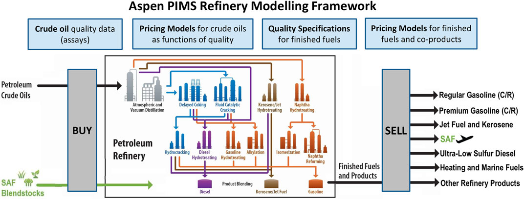
FIGURE 2. Refinery optimization model architecture with pricing, demand, and SAF blendstock property data flowing through PIMS model which generates optimal material and cash flows.

Several modifications were made to the refinery modelling framework presented in (Carlson et al., 2023) to better address the questions posed in this analysis.

- What is the expected value of a refiner investing capital to meet increasing jet demands?

- What is the expected value of a refiner integrating SAFs to meet increasing jet demands?

- What are the economic risks associated with each strategy from the refinery’s perspective given uncertainties in the oil and aviation industries?

- What incentive structures are most effective in mitigating said risks?

Modifications enabled discounted cash flow (DCF) analysis so that capital investments and future cash flows could be simultaneously considered with net present value (NPV) as a consistent metric. The intention was not to compute NPVs based on the whole refinery’s cash flows for either capital investment or SAF integration strategies. Instead, NPVs attributed to changes in refinery cash flows, from either capital investments or SAF purchases, were obtained by first running baseline cases and rerunning with pertinent changes in place. By analyzing only changes in performance, the influence of certain nuisances and assumptions inherent in the modeling framework were minimized, thereby improving the generality of results.

Moreover, DCF analysis was embedded into a broader Monte-Carlo framework to supplement economic viability calculations with some uncertainty quantification. A primary objective of the analysis was to elucidate the financial risks of SAF production, thereby providing insight into potential mitigation strategies should they be deemed necessary. The framework was designed to allow many simulations with random variables simulating market risks to be sampled efficiently and formatted as input to the refinery model (Meins and Sager, 2015). Resulting NPV distributions would then offer insights into the expected economic performance (weighted average), risks (standard deviation), and risk-adjusted performance (weighted average/standard deviation or Sharpe ratio) of each strategy.

The iterative procedure used to generate one Monte-Carlo simulation is described below alongside novel components of the modelling framework.

1) A jet debottlenecking strategy was first devised using refinery model constraints.

a. Capital Investment Strategy: Capacity expansion cost curves were incorporated into the modelling framework to assign costs to unit capacity increases representing potential capital projects a refinery could undergo to increase petroleum jet production.

b. SAF Integration Strategy: A SAF blendstock with a minimum blend volume was imposed to force the model’s integration of SAF.

2) Case management tools (external to PIMS) were developed to randomize Monte-Carlo variables representing uncertain market conditions and package 31 individual cases (corresponding to years 2020 through 2050) into a “simulation.”

3) A baseline refinery PIMS model, without a jet debottlenecking strategy implemented, was optimized for each of the 31 individual cases to have cash flows extracted.

4) The jet debottlenecking strategy was implemented via constraints and the PIMS model was reoptimized for each of the same 31 individual cases to have alternative cash flows extracted.

5) Baseline cash flows were subtracted from the jet debottlenecking strategy cash flows and entered into a DCF table.

a. Capital Investment Strategy: Investment costs were added to the DCF table and an NPV was calculated for the simulation.

b. SAF Integration Strategy: No investment costs were added to the DCF table and an NPV for the simulation was calculated based solely on future cash flows. Mitigation costs (MC) for SAF integration strategies were also calculated by solving for the SAF purchasing cost reduction needed to bring a simulation’s NPV to a target value.

A graphical depiction of the Monte-Carlo framework is provided in Figure 3 and more detailed descriptions of each modification to the original modelling framework described in (Carlson et al., 2023) are provided below.

FIGURE 3

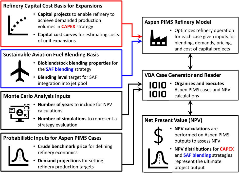
FIGURE 3. Monte-Carlo modelling framework used to generate NPV and MC distributions for capital investment and SAF integration strategies.

2.1 Capital expansion cost curves

The initial capacities of each unit operation were sized using the EIA’s 2020 Refinery Capacity Report to represent a large, high-conversion refinery located in the U.S. Gulf Coast (PADD3) region (Refinery Capacity Report, 2020). Although sweet crudes are typically processed in this region, a more diverse crude slate, with sour options, was modeled to expand the applicability of results. Furthermore, constraints were imposed to limit the purchased volumes of both sweet and sour crudes to a maximum of 50% of total capacity, respectively, thereby forcing the optimizer to consider both crude types. The inclusion of numerous conversion options (i.e., delayed coker, fluidized catalytic cracker, and hydrocracker) coupled with ample desulfurization capacity allowed the model to purchase both sweet and sour crude types without issue.

Developing a pricing basis for capacity expansion projects was necessary to analyze capital deployment scenarios refiners might consider in planning for changing product demands. The series of capital cost curves as a function of unit capacity shown in Figure 4 were sourced from literature (Gary et al., 2007) and updated to 2021 values by scaling plant cost indices to 2021 values (Chemical Engineering Plant Cost Index, 2022).

FIGURE 4

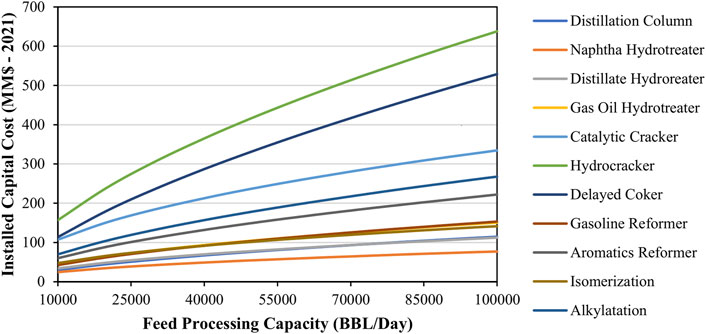
FIGURE 4. Refinery unit capital cost curves from literature (Gary et al., 2007).

These curves were fitted to power functions with factors ($F_i$) and exponents ($E_i$) where each $i$ denotes a different refinery unit. Power function parameters for each refinery unit shown in Figure 4 are tabularized in Table 1 in Supplementary Material alongside initial unit capacities. Each unit’s power function was used to calculate a capacity expansion cost, also referred herein as the installed capital cost (${ICC}_i$), as shown in Equation 1. It was assumed that the cost associated with increasing a unit’s capacity was approximated by the difference in cost of a newly constructed unit with the capacity achievable after expansion ($C_{i,f}$) and a newly constructed unit with the original capacity before expansion ($C_{i,0}$).

${\mathit{I}\mathit{C}\mathit{C}}_{\mathit{i}}={\mathit{F}}_{\mathit{i}}\left({{\mathit{C}}_{\mathit{i},\mathit{f}}}^{{\mathit{E}}_{\mathit{i}}}-{{\mathit{C}}_{\mathit{i},\mathbf{0}}}^{{\mathit{E}}_{\mathit{i}}}\right)(1)$

TABLE 1

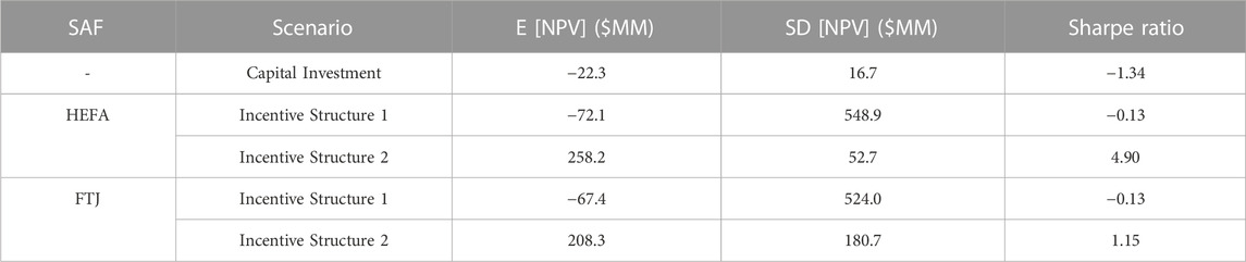
TABLE 1. Expected NPVs (E [NPV]), standard deviations (SD [NPV]), and Sharpe ratios (E [NPV]/SD [NPV]) for capital investment and SAF integration (subject to incentive structures 1 and 2) strategies.

2.2 Monte-Carlo variables

2.2.1 West Texas intermediate (WTI) crude price

The same crude/product pricing correlations to WTI price used in (Carlson et al., 2023) were also used in this analysis but WTI price was pulled from a distribution to simulate oil market volatility. WTI price was assumed to follow a log-normal distribution which implied the ratios of WTI prices year-over-year follow a normal distribution. The mean and standard deviation of historical year-over-year price ratios from 1990 to 2020 were used to define the distribution from which future price ratios were sampled from ($\mu$ = 1.06, $\sigma$ = 0.24). Lower and upper bounds were imposed at 42 and 157 $/bbl corresponding to the low and high oil price cases from EIA’s 2022 AEO (Annual Energy Outlook 2022, 2022). Figure 5 displays five sample WTI price projections which mirror the historical variability also shown for reference.

FIGURE 5

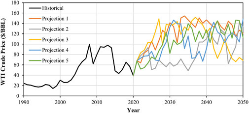
FIGURE 5. WTI crude price historical data alongside projections with identical stochastic movements.

2.2.2 Refinery product demand projections

Refinery product demand projections were based on EIA’s AEO 2022 update with one exception being that gasoline demands were overwritten with ADOPT projections. The ADOPT model was developed with support from the U.S. Department of Energy’s Vehicle Technology Office to estimate the impacts of technology improvements on light-duty vehicle sales and fuel consumption. When compared to EIA’s gasoline demand projections, the ADOPT model predicts a higher degree of vehicle electrification and a more pronounced decline in gasoline demand (Brooker et al., 2015). This projection was chosen to reflect a more challenging market trend for the refinery model to navigate.

In their AEO, EIA explicitly states demand projections “are not predictions of what will happen, but rather, they are modeled projections of what will happen given certain assumptions and methodologies (Annual Energy Outlook 2022, 2022).” Therefore, demands were considered as Monte Carlo input variables and were modelled with distributions. The AEO provided 8 projections resulting from different assumptions: high/low oil supply, high/low oil price, high/low economic growth, and high/low renewables cost (Annual Energy Outlook 2022, 2022). Oil supply, oil price, economic growth, and renewables cost were assumed to be orthogonal dimensions defining the space of possible demand projections for the purposes of this analysis. Oil price is a key input to ADOPT so high (157 $/bbl), low (42 $/bbl), and reference (83 $/bbl) oil price cases corresponding to AEO cases were modelled with the tool to quantify expected gasoline demands.

Three normally distributed random variables ($x_i$) where each $i$ corresponded to either the oil supply, economic growth, or renewables cost dimension were then used to represent the degree of influence each dimension had on a particular simulation. The random variables were set to range between −1 and +1 99.7% of the time with a mean value ($\mu$) of 0 and standard deviation ($\sigma$) of 0.33 using the empirical rule (2.2.7 - The Empirical Rule, 2022). The oil price dimension was treated separately since WTI prices were already sampled as described in section 3.2.1. WTI price trajectories were converted to a random variable by scaling ranges [42, 83] $/bbl to [-1, 0] and (83, 157] to (0, +1).

Furthermore, for each dimension, the difference in demand ($d$) for each product ($p$) and year ($y$) between the low and the reference case (${∆d}_{p,y,i,-}$) was linked to degree −1. Similarly, the difference between high and reference cases (${∆d}_{p,y,i,+}$) was linked to degree +1. The influence of each dimension was then determined using Equation 2 given random variable $x_i$.

${∆\mathit{d}}_{\mathit{p},\mathit{y},\mathit{i}}=\left\{\begin{array}{c}‖{\mathit{x}}_{\mathit{i}}‖{∆\mathit{d}}_{\mathit{p},\mathit{y},\mathit{i},-},{\mathit{x}}_{\mathit{i}}<\mathbf{0}\\ ‖{\mathit{x}}_{\mathit{i}}‖{∆\mathit{d}}_{\mathit{p},\mathit{y},\mathit{i},+},{\mathit{x}}_{\mathit{i}}\ge \mathbf{0}\end{array}\right.(2)$

Normal distributions were chosen for oil supply, economic growth, and renewables cost dimensions to give a natural preference to the reference case which was represented by the mean for each dimension. The influences of each of the four dimensions were then added to the reference case demand ($d_{ref}$) for each product and year as shown in Equation 3.

${\mathit{d}}_{\mathit{p},\mathit{y}}={\mathit{d}}_{\mathit{r}\mathit{e}\mathit{f},\mathit{p},\mathit{y}}+{\displaystyle \sum _{\mathit{i}=\mathbf{1}}^{\mathbf{4}}}{∆\mathit{d}}_{\mathit{p},\mathit{y},\mathit{i}}(3)$

Each demand projection was determined as the summation of random degrees of influence from oil supply, oil price, economic growth, and renewables cost ranging between the high/low scenarios provided in the AEO with gasoline demands provided by ADOPT.

3 Results

3.1 Capital investment

3.1.1 Debottlenecking

To understand what unit expansions and associated costs a hypothetical refiner might undergo to meet future fuel demands, it was first necessary to locate where refinery bottlenecks might develop. Monte Carlo demand variables were fixed to +1 to simulate a maximum jet demand scenario where the likelihood of bottlenecking would be highest. Note that SAF blending was not permitted in these cases. Production turndowns resulting from low margins were avoided by setting the WTI benchmark to its lower bound ($42/bbl) where margins were found to be highest in (Carlson et al., 2023). Figure 6 stacks the anticipated refinery product demands for the maximum jet scenario, resulting refinery model product supply limitations, and refinery unit sub-model capacity utilizations over time.

FIGURE 6

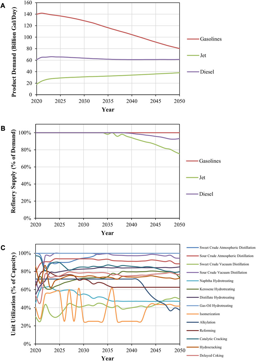
FIGURE 6. (A) EIA’s maximum-jet and diesel demand projections from 2022 AEO with corresponding ADOPT gasoline demand projections (B) Percentage of projected demand supplied by the refinery optimization model. Anything less than 100% indicates a bottleneck (C) Individual refinery unit capacity utilizations.

As shown in Figure 6B, the refinery model satisfied market demands until jet supply in 2034 and diesel supply in 2040 started deviating. Therefore, the model predicted a production bottleneck for C9-C28 hydrocarbons that would likely result in insufficient supply of jet or diesel.

The refinery unit sub-model utilizations in Figure 6C were used to pinpoint the anticipated bottlenecks responsible for the jet/diesel supply constraint. From 2020 to 2050, both the sweet crude atmospheric distillation column and gas-oil hydrotreater capacities were fully utilized indicating potential unit bottlenecks. Consequently, these unit capacities were arbitrarily increased while rerunning the 2050 case to determine what throughputs the model would need to satisfy market demands. The year 2050 was chosen because it represented the greatest shift in demands relative to the 2020 case. Upon further investigation, the model utilized 197,500 bbl/day and 91,600 bbl/day of sweet crude atmospheric distillation and gas-oil hydrotreating capacity, respectively, so marginally higher capacities (200,000 and 95,000 bbl/day) were implemented in 2034. The original capacities for these units were 130,000 bbl/day and 72,000 bbl/day implying 53% and 32% increases. Re-running cases from 2020 to 2050 confirmed the refinery model could always meet gasoline, jet, and diesel demand with the expansions implemented. The atmospheric distillation and gas-oil hydrotreater capacities were decreased by a factor of 10/12 in 2033 to account for 2 months of turnaround downtime over the 12-month period in 2033.

3.1.2 Financial performance

The Monte Carlo input variables were unfixed from baselining and 100 random samplings of WTI prices and product demands were fed to the model to compute the distribution of economic performance (NPVs) displayed in Figure 7.

FIGURE 7

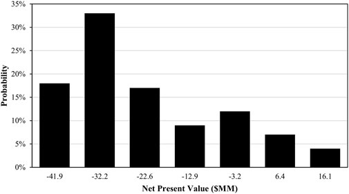
FIGURE 7. Distribution of NPVs achieved by the CAPEX strategy developed earlier over 100 random samplings of economic conditions.

Figure 7 indicates a high probability the expansion projects would be an unattractive investment with high uncertainty. The expected value for NPV, calculated as the weighted average between NPVs and probabilities, was found to be $-22.3 million and was considered a benchmark for economic performance in strategies to follow. The Sharpe Ratio, calculated as the expected NPV divided by the standard deviation of NPVs observed, was found to be −1.34.

3.2 SAF integration

The model was reconfigured to purchase a drop-in SAF to un-constrain jet production while disregarding the capital investments previously outlined. Although many feedstocks are being considered for SAF production, two were analyzed with independent simulation sets to compare results given significantly different purchasing prices and blending properties while limiting computational requirements.

Hydrogenated Esters and Fatty Acids (HEFA) were selected as the first SAF because of market readiness and authorization from CORSIA/ASTM to be blended up to 50 volume % (Tao et al., 2017). More specifically, jatropha sourced HEFA was chosen for its low cost, assumed to be $3.82/gal with nth plant assumptions, to represent a relatively economical option for refinery integration compared to other SAFs (Tao et al., 2017). Fischer-Tropsch Jet (FTJ) was selected as the second SAF because of its equal authorization from CORSIA and greater scalability potential when compared to HEFA, with a broader array of compatible feedstocks such as woody biomass, agricultural residues, or municipal solid waste (Alexander et al., 2012). FTJ’s higher purchasing price of $5.03, corresponding to woody forestry resides as feedstock, also presented a significantly higher price point for the refinery model to accommodate (Capaz et al., 2021).

The model was constrained to blend each SAF at 25 volume % while producing all demanded jet fuel. This constraint was required because the relatively high purchasing prices assumed here never provided a natural incentive for the refinery to purchase SAF over more crude oil.

3.2.1 Financial performance

Another 100 simulations were passed through the model to determine NPVs associated with SAF integration. Subsequently, the required SAF cost reduction per gallon, termed mitigation cost (MC), necessary to bring the simulation NPV to parity with the expected capital investment strategy NPV of $-22.3 million was determined for each of the 100 simulations. The distribution of mitigation costs needed for HEFA and FTJ are shown in Figures 8A,B, respectively.

FIGURE 8

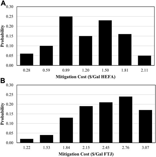
FIGURE 8. Distribution of mitigation costs needed to bring each simulation’s NPV to $-22.3 million (on-par with the expected NPV of the capital projects strategy) for (A) HEFA and (B) FTJ.

The expected value of mitigation costs required to achieve parity with the capital investment benchmark NPV, calculated as the weighted average of observed mitigation costs and probabilities, were found to be $1.22/gal for HEFA and $2.43/gal for FTJ. For reference, mitigation costs available from combing California’s Low Carbon Fuel Standard (LCFS) credit and Renewable Identification Numbers (RINs) are $2.70/gal for HEFA and 3.54 $/gal for FTJ as calculated in the Supplementary Material (US EPA, 2015; California Low Carbon Fuel Standard Credit price, 2017; US EPA, 2018). While this study does not prescribe where such mitigation costs should come from, a combination of feedstock cost reductions, technology improvements, and SAF purchasing incentives could be combined to reach the mitigation cost needed and match the financial performance of the capital investment scenario (NPV of $-22.3 million).

3.2.2 Hypothetical incentive structure 1

To model a hypothetical incentive structure, expected mitigation costs were deducted from original purchasing prices assumed in the refinery model. Both HEFA and FTJ prices were consequently reduced to $2.60/gal ($109/bbl), a much more viable price considering the WTI price sampling distribution ranging from 42—157 $/bbl. The fact both HEFA and FTJ expected mitigation costs reduced each SAF to the same price indicated $2.60/gal was a common price the model would pay for a jet blendstock instead of undergoing the capital investment strategy outlined in Section 4.1.1.

According to one study, HEFA sourced from jatropha oil is estimated to emit 36%–52% of the CO₂ emissions compared to fossil jet (Wang et al., 2016). Using an average of 44% (i.e. 56% CO₂ emissions reduction), a fossil jet energy density of 132 MJ/gal, a HEFA energy density of 121 MJ/gal, and assuming fossil jet to have life cycle emissions of 89 gCO₂e/MJ, the amount of carbon emissions saved per gallon of HEFA blended over fossil jet was calculated in Equation 4 (11, 23). Combining the carbon emissions saved per gallon with the expected mitigation cost of $1.22/gal from section 4.2.1 yielded the marginal abatement cost (MAC) of CO₂ associated with HEFA in Equation 5.

${∆CO}_{2e,HEFA}=\left(\frac{89g{CO}_{2e}}{MJ}\bullet \frac{132MJ}{Gal}-\frac{\left(0.44\right)89gC{O}_{2e}}{MJ}\bullet \frac{121MJ}{Gal}\right)\bullet \frac{1Ton}{907185g}=7.8e-3\frac{Ton{CO}_{2e}}{Gal}(4)$

${MAC}_{HEFA}=\frac{Gal}{7.8e-3Ton{CO}_{2e}}\bullet \frac{\$2.37}{Gal}=158\frac{\$}{Ton{CO}_{2e}}(5)$

The emissions reduction of FTJ over fossil jet is estimated to be 96% (Capaz et al., 2021). Similarly, carbon emissions saved per gallon and an associated MAC were calculated for FTJ in Eqs (6, (7 using the expected mitigation cost of $2.43/gal determined in section 4.2.1.

${∆CO}_{2e,FTJ}=\left(\frac{89g{CO}_{2e}}{MJ}\bullet \frac{132MJ}{Gal}-\frac{\left(0.96\right)89gC{O}_{2e}}{MJ}\bullet \frac{121MJ}{Gal}\right)\bullet \frac{1Ton}{907185g}=1.2e-2\frac{Ton{CO}_{2e}}{Gal}(6)$

${MAC}_{FTJ}=\frac{Gal}{1.2e-2Ton{CO}_{2e}}\bullet \frac{\$3.58}{Gal}=195\frac{\$}{Ton{CO}_{2e}}(7)$

Another randomized set of 100 samples was generated with the mitigated SAF prices to generate the distributions of NPVs shown in Figures 10A,B.

3.2.3 Hypothetical incentive structure 2

Looking back on the mitigation costs needed to bring integrating SAF to parity with the expected capital investment strategy NPV, a strong correlation to average WTI price was observed. Figure 9 displays the inverse relationships between the average of all WTI prices observed in each 31-year window and the calculated mitigation cost, for HEFA and FTJ, across those 31 years Figure 9 confirms the intuition that lower crude prices require more mitigation to compensate for the opportunity cost of not purchasing more inexpensive crude oil.

FIGURE 9

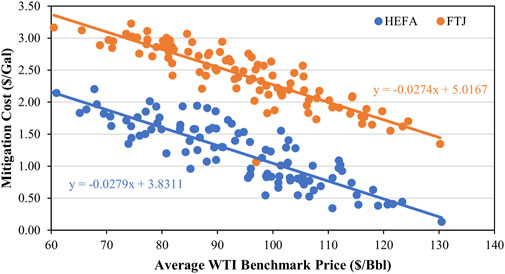
FIGURE 9. Mitigation cost reductions needed for HEFA purchases to bring each NPV to $-22.3 million plotted against average WTI price for each simulation.

Another hypothetical incentive structure was implemented where the mitigation cost applied to the SAF purchasing price varied with WTI benchmark price. The linear least squares regression lines shown in Figure 9 were used as proxies to establish dependencies between WTI prices and mitigation costs. Consequently, HEFA and FTJ prices were calculated using Eq. 8, Eq. 9 for each year depending on the sampled WTI benchmark price (P_WTI) in $/bbl.

$P_{HEFA\frac{\$}{gal}}=3.82-\left[-0.03P_{WTI,\frac{\$}{bbl}}+3.83\right](8)$

$P_{FTJ\frac{\$}{gal}}=5.03-\left[-0.03P_{WTI,\frac{\$}{bbl}}+5.02\right](9)$

Additional sets of 100 random samples were drawn with Eq. 8, Eq. 9 determining HEFA and FTJ purchasing prices, respectively. Resulting NPV distributions are documented in Figures 10A,B alongside the distributions generated from the capital investment strategy in section 4.1.2 and Incentive Structure 1 in section 4.2.1. Expected NPVs, standard deviations, and Sharpe ratios are shown in Table 1.

FIGURE 10

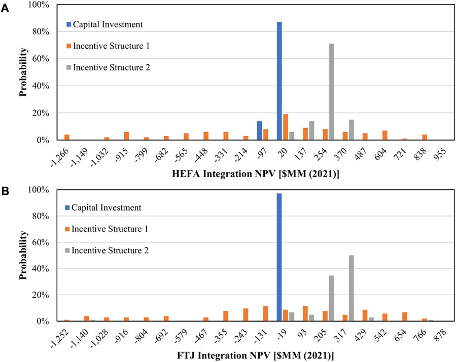
FIGURE 10. NPVs observed over 100 random samplings of economic conditions for the capital investment strategy, SAF integration with fixed mitigation costs deducted (Incentive Structure 1), and SAF integration with variable mitigation costs deducted (Incentive Structure 2) for (A) HEFA and (B) FTJ. Note that the capital investment distributions in (A) and (B) are identical to those found in Figure 7 and the scaling of the x-axis causes a visual discrepancy.

Total marginal abatement costs of CO₂ (MAC), computed as the summed cost of mitigation divided by the summed CO₂ emission savings, over each 31-year window composing each simulation were calculated for Incentive Structures 1 and 2. The distributions of MACs attributed to integrating HEFA and FTJ are shown in Figures 11A,B.

FIGURE 11

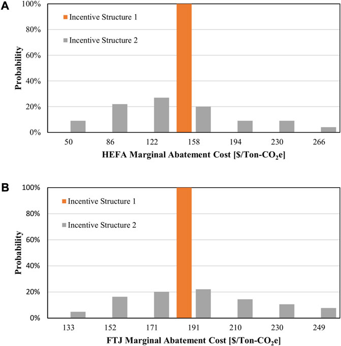
FIGURE 11. Distributions of marginal abatement costs ($/Ton-CO₂e), calculated for each simulation as total cost of mitigation divided by total emissions saved, for both (A) HEFA and (B) FTJ.

4 Discussion

Results indicate that refineries deploying capital to produce more fossil jet fuel is a risky proposition given the uncertainties present in the market as evidenced by Figure 10. Moreover, the distribution of mitigation costs shown in Figure 8 indicate that directly blending SAFs with refinery jet blendstocks is probably economically viable given current incentives likes LCFS and RIN credits. More specifically, producing SAFs with sufficiently low production costs and high carbon intensity reductions, thereby generating more LCFS credits, can be profitable if the final price is approximately $2.60/gal, given the specifics presented in this analysis.

However, a comparison between the capital investment and Incentive Structure 1 strategy distributions in Figure 10 highlights the inherent risk that biofuel producers take on when their business is supported with fixed incentives within the context of greater market volatility. Even when mitigating 32% of the HEFA cost, or 49% of the FTJ cost, the variability in economic outcomes resulting from Incentive Structure 1 observed in Figure 10 would likely be considered too risky to invest in SAF integration projects. Alternatively, both quantitively (Table 1) and qualitatively (Figure 10), Incentive Structure 2 clearly produces a preferable distribution of economic outcomes when compared to Incentive Structure 1. Incentive Structure 2 removes much of the risk associated with Incentive Structure 1 and even overcompensates in terms of expected NPV for both HEFA and FTJ integration scenarios.

Yet, it is important to note where risk is borne in the case of Incentive Structure 2, as the underlying sources of uncertainty are still present. To reiterate, mitigation costs could be composed of feedstock cost reductions, technology improvements, and SAF purchasing incentives. Both feedstock cost reductions and technology improvements are longer-term trends that are not freely changed in step with oil market volatility. Therefore, any variability in mitigation costs would likely need to come from a sufficiently large fund that supplies mitigation credits when oil prices are low and collects debits when oil prices are high. The fund would effectively serve as an economic buffer to absorb risk for SAF producers, refiners, and airline companies. The key difference between current biofuel incentive structures, represented by Incentive Structure 1, and the proposed fund, represented by Incentive Structure 2, is the introduction of bidirectional payments.

The question of how efficient Incentive Structure 2 was compared to Incentive Structure 1 then arose, or in other words, how did resulting MACs compare? The expected MAC for HEFA observed in Figure 11A was $136/Ton-CO2e which was 13% lower than the fixed MAC ($156/Ton-CO2e) attributed to Incentive Structure 1. Similarly, Figure 11B implied an expected MAC of $182/Ton-CO2e for FTJ which was 7% lower than the fixed Inventive Structure 1 MAC of $195/Ton-CO2e. For both SAFs, the total, long-term cost of providing variable rather than fixed incentives was lower.

It is also worth noting the variable mitigation cost formulas (Equations (8 and (9) implemented in Incentive Structure 2 both exceeded the economic performance target, being the expected NPV for the capital projects strategy, as evidenced by Figures 10A,B. Refined mitigation cost formulas that more closely matched the capital investment strategy NPV would likely bring the expected MACs attributed to Incentive Structure 2 down even further while still more effectively de-risking SAF production for industry adoption.

5 Conclusion

In summary, preexisting refinery optimization models were further developed to consider capital investments and market risks via Monte-Carlo simulation. The resulting framework enabled economic value and risk comparisons between refinery investments to produce more petroleum jet and SAF integration to meet rising jet demands. This framework could be leveraged to address similar questions faced by refiners interested in balancing future investments with decarbonization goals.

Two distinct SAF purchasing incentive structures were also tested within the modelling framework. A traditional, fixed incentive per volume of SAF, was shown to produce untenable economic risk for SAF producers and refiners to sustainably integrate. Results indicated that variably incentivizing SAF purchases in step with changing crude oil prices could be a more efficient and effective way to support SAF deployment relative to fixed incentive structures.

The concept of market-sensitive, variable incentives could hypothetically be generalized to any biofuel being integrated into existing fossil-fuel markets which are more mature and accordingly able to absorb risk. Moreover, support from an effective incentive structure will allow SAF or other biofuel producers to more quickly gain the operating experience needed to realize nth plant prices thereby reducing broader decarbonization timelines. For these reasons, mitigating pricing risks upfront as suggested here, in a fair and sustainable way could be integral to the growth of the SAF and greater biofuels industries.

Data availability statement

The raw data supporting the conclusion of this article will be made available by the authors, without undue reservation.

Author contributions

NC, MT, and AS were responsible for conceptualizing the analysis and methods. NC and MT developed the modelling framework expansions detailed in the methods section and generated resulting data and figures. NC created the original draft manuscript. AS, LT, and RD performed an extensive review and edit to prepare the manuscript for publication. All authors contributed to the article and approved the submitted version.

Funding

This work was authored in part by the National Renewable Energy Laboratory, operated by Alliance for Sustainable Energy, LLC, for the U.S. Department of Energy (DOE) under Contract No. DE-LC-000L054. The views expressed in the article do not necessarily represent the views of the DOE or the U.S. Government. The U.S. Government retains and the publisher, by accepting the article for publication, acknowledges that the U.S. Government retains a nonexclusive, paid-up, irrevocable, worldwide license to publish or reproduce the published form of this work, or allow others to do so, for U.S. Government purposes.

Conflict of interest

The authors declare that the research was conducted in the absence of any commercial or financial relationships that could be construed as a potential conflict of interest.

Publisher’s note

All claims expressed in this article are solely those of the authors and do not necessarily represent those of their affiliated organizations, or those of the publisher, the editors and the reviewers. Any product that may be evaluated in this article, or claim that may be made by its manufacturer, is not guaranteed or endorsed by the publisher.

Supplementary material

The Supplementary Material for this article can be found online at: https://www.frontiersin.org/articles/10.3389/fenrg.2023.1223874/full#supplementary-material

References

Alexander, Z., Scheuermann, S., and Ortner, J. (2012). ‘High Biofuel Blends in Aviation (HBBA)’. Deutsche Lufthansa AG and Wehrwissenschaftliches Institut Fur Werk-und Betriebsstoffe. Available at: https://ec.europa.eu/energy/sites/ener/files/documents/final_report_for_publication.pdf (Accessed: April 21, 2022).

Google Scholar

Annual Energy Outlook 2022 (2022). U.S. Energy information administration (EIA). Available at: https://www.eia.gov/outlooks/aeo/index.php (Accessed: March 6, 2023).

Google Scholar

Aviation (2022). Paris: iea. Available at: https://www.iea.org/reports/aviation (Accessed: April 21, 2022).

Google Scholar

Boyd, R. (2022). Sustainable aviation fuel: technical certification international air transportation association. Available at: https://www.iata.org/contentassets/d13875e9ed784f75bac90f000760e998/saf-technical-certifications.pdf.

Google Scholar

Brooker, A., Gonder, J., and Ward, J. (2015). “Adopt: A historically validated light duty vehicle consumer choice model,” in SAE 2015 world congress and exhibition (Detroit, Michigan: SAE). doi:10.4271/2015-01-0974

CrossRef Full Text | Google Scholar

California Low Carbon Fuel Standard Credit price (2017). Neste worldwide. Available at: https://www.neste.com/investors/market-data/lcfs-credit-price (Accessed: August 16, 2022).

Google Scholar

Capaz, R. S., Guida, E., Joaquim, E. A., Osseweijer, P., and Posada, J. A. (2021). Mitigating carbon emissions through sustainable aviation fuels: costs and potential. Biofuels, Bioprod. Biorefining 15 (2), 502–524. doi:10.1002/bbb.2168

CrossRef Full Text | Google Scholar

Carlson, N. A., Singh, A., Talmadge, M. S., Jiang, Y., Zaimes, G. G., Li, S., et al. (2023). Economic analysis of the benefits to petroleum refiners for low carbon boosted spark ignition biofuels. Fuel 334, 126183. doi:10.1016/j.fuel.2022.126183

CrossRef Full Text | Google Scholar

Chemical Engineering Plant Cost Index (2022). Chemical engineering. Available at: https://www.chemengonline.com/pci (Accessed: April 22, 2022).

Google Scholar

Chiaramonti, D. (2019). Sustainable aviation fuels: the challenge of decarbonization. Energy Procedia 158, 1202–1207. doi:10.1016/j.egypro.2019.01.308

CrossRef Full Text | Google Scholar

Climate Change Mitigation: CORSIA (2019). International Civil aviation organization. Available at: https://www.icao.int/environmental-protection/CORSIA/Documents/ICAO%20Environmental%20Report%202019_Chapter%206.pdf (Accessed: April 21, 2022).

Google Scholar

Commercial Aerospace Insight Report (2021). Accenture. Available at: https://www.accenture.com/_acnmedia/PDF-151/Accenture-Commercial-Aerospace-Insight-Report-2021.pdf (Accessed: April 22, 2022).

Google Scholar

Commercial Market Outlook 2019-2038 (2019). Boeing. Available at: https://www.boeing.com/resources/boeingdotcom/commercial/market/commercial-market-outlook/assets/downloads/cmo-sept-2019-report-final.pdf (Accessed: April 22, 2022).

Google Scholar

Driessen, C., and Hak, M. (2021). Electric flight in the Kingdom of The Netherlands. Netherlands airport consultants (NACO). Available at: https://www.rijksoverheid.nl/binaries/rijksoverheid/documenten/rapporten/2022/02/18/bijlage-1-masterplan-electric-flight-naco-nlr-short-report/bijlage-1-masterplan-electric-flight-naco-nlr-short-report.pdf.

Google Scholar

Future of Aviation (2019). International Civil aviation organization. Available at: https://www.icao.int/Meetings/FutureOfAviation/Pages/default.aspx (Accessed: April 21, 2022).

Google Scholar

Gary, J. H., Handwerk, G. E., and Kaiser, M. J. (2007). Petroleum refining technology and economics. Boca Raton, FL: CRC Press Taylor & Francis Group, LLC.

Google Scholar

Global downstream outlook to 2035 (2019). McKinsey. Houston, TX: McKinsey & Company.

Google Scholar

Global Market Forecast 2019-2038 (2019). France: airbus. Available at: https://www.airbus.com/sites/g/files/jlcbta136/files/2021-07/GMF-2019-2038-Airbus-Commercial-Aircraft-book.pdf (Accessed: April 22, 2022).

Google Scholar

Gössling, S., and Humpe, A. (2020). The global scale, distribution and growth of aviation:implications for climate change. Glob. Environ. Change 65, 102194. doi:10.1016/j.gloenvcha.2020.102194

PubMed Abstract | CrossRef Full Text | Google Scholar

Holladay, J., Abdullah, Z., and Heyne, J. (2020). Sustainable aviation fuel: review of technical pathways. U.S. Department of energy Office of energy efficiency and renewable energy Bioenergy technologies Office. Available at: https://www.energy.gov/sites/default/files/2020/09/f78/beto-sust-aviation-fuel-sep-2020.pdf (Accessed: June 26, 2023).

Google Scholar

Jiang, Y., Zaimes, G. G., Li, S., Hawkins, T. R., Singh, A., Carlson, N., et al. (2023). Economic and environmental analysis to evaluate the potential value of co-optima diesel bioblendstocks to petroleum refiners. Fuel 333, 126233. doi:10.1016/j.fuel.2022.126233

CrossRef Full Text | Google Scholar

Meins, E., and Sager, D. (2015). Sustainability and risk: combining Monte Carlo simulation and DCF for Swiss residential buildings. J. Eur. Real Estate Res. 8 (1), 66–84. doi:10.1108/JERER-05-2014-0019

CrossRef Full Text | Google Scholar

Newsom, R., Murphy, B., and Ram, R. (2023). Sustainable aviation fuel (SAF) on the rise: Sustainable development through a dynamic environment. London, United Kingdom: Ernst & Young LLP.

Google Scholar

Paris Agreement (2015). United nations. Available at: https://unfccc.int/sites/default/files/english_paris_agreement.pdf (Accessed: April 21, 2022).

Google Scholar

Refinery Capacity Report (2020). U.S. Energy information administration. Available at: https://www.eia.gov/petroleum/refinerycapacity/(Accessed December 1, 2020).

Google Scholar

Rep Yarmuth, J. A. (2022). Inflation reduction act of 2022. Available at: http://www.congress.gov/bill/117th-congress/house-bill/5376 (Accessed: June 22, 2023).

Google Scholar

SAF Grand Challenge Roadmap (2022). U.S. Department of energy, U.S. Department of transportation, and U.S. Department of agriculture, in collaboration with the U.S. Environmental protection agency. Available at: https://www.energy.gov/sites/default/files/2022-09/beto-saf-gc-roadmap-report-sept-2022.pdf.

Google Scholar

Schwab, A., Thomas, A., and Bennett, J. (2021). Electrification of aircraft: Challenges, barriers, and potential impacts. Golden, CO: National Renewable Energy Laboratory. doi:10.2172/1827628

CrossRef Full Text | Google Scholar

Shahriar, M. F., and Khanal, A. (2022). The current techno-economic, environmental, policy status and perspectives of sustainable aviation fuel (SAF). Fuel 325, 124905. doi:10.1016/j.fuel.2022.124905

CrossRef Full Text | Google Scholar

Soone, J. (2022). ‘ReFuelEU aviation initiative’. European parliamentary research service. Available at: https://www.europarl.europa.eu/RegData/etudes/BRIE/2022/729457/EPRS_BRI(2022)729457_EN.pdf.

Google Scholar

Su, J., van Dyk, S., and Saddler, J. (2022). Repurposing oil refineries to “stand-alone units” that refine lipids/oleochemicals to produce low-carbon intensive, drop-in biofuels. J. Clean. Prod. 376, 134335. doi:10.1016/j.jclepro.2022.134335

CrossRef Full Text | Google Scholar

Tanzil, A. H., Brandt, K., Zhang, X., Wolcott, M., Stockle, C., and Garcia-Perez, M. (2021). Production of sustainable aviation fuels in petroleum refineries: evaluation of new bio-refinery concepts. Front. Energy Res. 9, 735661. doi:10.3389/fenrg.2021.735661

CrossRef Full Text | Google Scholar

Tao, L., Milbrandt, A., Zhang, Y., and Wang, W. C. (2017). Techno-economic and resource analysis of hydroprocessed renewable jet fuel. Biotechnol. Biofuels 10 (1), 261. doi:10.1186/s13068-017-0945-3

PubMed Abstract | CrossRef Full Text | Google Scholar

The Empirical Rule (2022). STAT 200 | elementary statistics. Available at: https://online.stat.psu.edu/stat200/lesson/2/2.2/2.2.7 (Accessed: April 22, 2022).

Google Scholar

US EPA (2015). Approved pathways for renewable fuel. Available at: https://www.epa.gov/renewable-fuel-standard-program/approved-pathways-renewable-fuel (Accessed August 16, 2022).

Google Scholar

US EPA (2018). RIN trades and price information. Available at: https://www.epa.gov/fuels-registration-reporting-and-compliance-help/rin-trades-and-price-information (Accessed August 16, 2022).

Google Scholar

Wang, W. C., Tao, L., and Markham, J. (2016). Review of biojet fuel conversion technologies. Golden, CO (United States): National Renewable Energy Lab. NREL. doi:10.2172/1278318

CrossRef Full Text | Google Scholar