Geospatial segmentation of high-resolution photovoltaic production maps for Switzerland

1 Introduction

The share of solar energy in the global renewable energy mix is growing, and it is expected to be the leading source by 2050 (International Energy Agency, 2022). The same holds for Switzerland. But to reach the declared goal of net-zero CO₂ emission by 2050 (Swiss Federal Office of Energy, 2020), annual increase in PV capacity needs to speed up significantly. Until recently, politics and subsidy structures focused almost exclusively on roof-top installations with a high level of auto consumption (Haelg et al., 2022). Large-scale, free-standing installations were highly disfavored: 1) It was almost impossible to get a building permit for a free-standing PV installation outside the building zone, i.e., anywhere outside urban areas. 2) There was a strong opposition from landscape protection activists and environmental protection agencies. 3) Lack of subsidies and low feed-in tariffs prevented economic viability. As a result, the newly installed PV capacity stayed far behind what is required to meet energy transition goals. In 2022, geopolitical conditions and the threat of a winter energy shortage have radically altered the terms of the debate. With unprecedented speed and almost no opposition, an adaptation to the existing energy law was passed on 30th of September, 2022. It has come into practice on the 1st of October and will remain valid until 31st of December, 2025 (Energiegesetz, 2022). With the exception of a few protected areas, utility scale PV installations can now be built outside the building zone and—given certain constraints—will be subsidized with up to 60% of the capital expenditure. They will be given priority over landscape protection and several other interests and are declared to be “of national interest.” This change in legislation has precipitated an enormous rush amongst electricity companies, communities and private investors to initiate new PV projects. The competition is tough and the timelines extremely tight. The subsidies for large PV installations will be given on a first-come first-served basis and will stop once the subsidized capacity is estimated to produce 2 TWh/year. Another ambitious requirement is that 10% of the future installation need to be connected to the grid by the end of 2025. Given delivery times of 1.5–2 years for major electrical components such as inverters and transformers (Hitachi and Siemens, 2023) and admission procedures for grid reinforcement (Swissgrid, 2022) this is almost impossible. The questions at the moment are thus: 1. What type of areas are currently available for PV installations in Switzerland? 2. Where are those areas and how large are they? 3. What is their production potential and how much of it is produced in winter?

Several studies have assessed the available surface area of different landcover types and published their associated energy production potential. Since the installations on houses had been largely prioritized in the past, a comprehensive dataset called Sonnendach and its twin study Sonnenfassade have been published by the Swiss Federal Office of Energy (Swiss Federal Office of Energy, 2022a; Swiss Federal Office of Energy, 2022b). Based on these datasets, several studies computed the rooftop potential under various exclusion assumptions (Gutschner et al., 2002; Gutschner, 2006; Cattin et al., 2012; Buffat et al., 2017; Remund, 2017; Bartlett et al., 2018; Portmann et al., 2022; Remund, 2019; Remund, 2020; Walch et al., 2018; Moro et al., 2021; Anderegg et al., 2022; Walch, 2022). The results deviate largely due to the different approaches and assumptions these studies have taken. A meta study from the national industry-academia consortium SWEET-EDGE (SWEET EDGE, 2023) disemminates the pool of studies and harmonizes the diverse results (Bucher et al., 2023). The potential of facades has been estimated by (Gutschner et al., 2002; Remund, 2017; Remund, 2019; Portmann et al., 2022).

PV installations in combination with agriculture may—under the requirement of improved yield—also qualify for building permits and subsidies according to the new energy law. Its potential was studied by Jaeger et al. (2022). Alpine regions have also been assessed for their energy potential (Kahl et al., 2018; Remund 2019; Egli et al. 2022; Meyer et al., 2023), but it is particularly difficult to compare those results because the criteria for what is considered feasible as installation locations are very diverse. The potential of artificial reservoirs was studied by Maddalena et al. (2022) and a suggestion for installations on natural lakes was made by Wanner et al. (2022).

A common feature of all these studies is that while a large number of geospatial and technical criteria are applied and discussed in great depth, the foundational surface radiation datasets used in these studies remain quite coarse. In most cases, the radiation values are known only at kilometer-scale. This resolution is unsuitable for studies in areas of complex mountainous topography such as the Alps, which incidentally cover vast areas of the Swiss territory.

In this study, we introduce a novel set of surface radiation calculations at an unprecedented resolution of 25 m throughout the Swiss territory. Next, we convert these base radiation maps to solar-yield potential for different solar PV tilt angles. Optimal tilt angles for each pixel are calculated to maximize either annual or winter production. Finally, using these high-resolution radiation maps, we perform a ‘high-level’ geospatial-segmentation of the yield potential into two major groups with two sub-groups each. These are 1) Agricultural land with sub-groups of permanent farm land and summer grazing land and 2) Water bodies, with sub-groups of natural and artificial water bodies. Additionally, rooftop solar yield is aggregated nationally to provide a baseline value for comparison.

The following sections are organized as follows. Section 2 discusses the preparation of the surface radiation maps as well as the solar yields. The following Section 3 discusses the results in terms of solar yield potential for each geospatial sub-group. The final section draws conclusions and future work.

2 Methods

2.1 Base radiation maps

The base radiation maps consist of surface radiation variables such as global horizontal irradiance (GHI), direct normal irradiance (DNI) and diffuse horizontal irradiance (DHI) at a 25 m resolution. They are derived using the Heliomont algorithm developed at Meteoswiss. Heliomont uses satellite data from the Meteosat family (Schmetz et al., 2002) to calculate the radiative forcing of clouds, i.e., it estimates the properties of the clouds that determine how much of the incoming solar radiation will be absorbed by them. Combining this information with pre-computed clear-sky irradiance and with radiative impacts of atmospheric aerosol, water vapor and ozone, Heliomont then estimates the amount of solar radiation that reaches the surface of the earth. The algorithm further includes a snow-cloud discrimination which sets it apart from most other radiation products and makes it particularly suitable for the alpine areas.

The most notable aspect of our work is to translate the radiation products from the satellite’s native grid resolution of 1.6 × 2.3 km to an extremely high resolution of 25 × 25 m. To achieve this translation, the following steps are taken:

• Re-run Heliomont to produce “horizon-free” surface radiation maps. The topographic effects, namely, shadows and blocking of the “sky” hemisphere are not taken into account in this simulation.

• Calculate horizons using a digital elevation model (DEM) of the required resolution. In this case, the EUDEM v1.1 is used. The horizons are calculated using the algorithm in Dozier and Frew (Dozier and Frew, 1990) at an azimuthal interval of 1°. Thus, for the entire swiss territory, 360 values of horizons are computed at 25 m resolution.

• Further, the skyview factor for each pixel is calculated using, once again, the formulation in Dozier and Frew.

• The horizon-free products computed in step 1 above are reprojected and matched to the high-resolution 25 m grid using bilinear interpolation.

• Shadows using horizon maps in the step above are imposed to calculate DNI at high resolution

• Skyview factors in the above step are used to calculate DHI at high resolution.

2.2 Energy yield

Once the incoming solar radiation maps are prepared as described in Section 2.1, the first step in deriving power yield estimates is calculating Plane-of-Array (POA) irradiation values. While we follow the well-known methodology of calculating POA as found in textbooks, for example, Iqbal (2012), we have stated it in a slightly different manner to be closer to how the calculations are actually performed and while conforming to the calculation details described in the previous section.

In this study, we compute energy yield from a standard monofacial solar PV panel. The POA irradiation is a sum of the contributions from direct, diffuse and reflected solar radiation,

$\mathrm{P}\mathrm{O}\mathrm{A}={\mathrm{P}\mathrm{O}\mathrm{A}}_{\mathit{Direct}}+{\mathrm{P}\mathrm{O}\mathrm{A}}_{\mathit{Diffuse}}+{\mathrm{P}\mathrm{O}\mathrm{A}}_{\mathit{Reflected}}(1)$

$\begin{array}{ll}\hfill {\mathrm{P}\mathrm{O}\mathrm{A}}_{\text{Direct}}\left(x,y\right)& ={\displaystyle \sum _{i=1}^N}DN{I}_{nh}\left(x,y,{\left({\theta }_{\mathit{sun}},{\varphi }_{\mathit{sun}}\right)}_i\right)\cdot f\left(\left({\theta }_P,{\varphi }_P\right),{\left({\theta }_{\mathit{sun}},{\varphi }_{\mathit{sun}}\right)}_i\right)\hfill \\ \hfill & \cdot S\left(x,y,{\left({\theta }_{\mathit{sun}},{\varphi }_{\mathit{sun}}\right)}_i\right)\hfill \end{array}(2)$

where DNI is a function of the 2D geospatial location $\left(x,y\right)$ and the sun position $\left({\theta }_{\mathit{sun}},{\varphi }_{\mathit{sun}}\right)$, f is a geometric factor that describes the panel orientation $\left({\theta }_P,{\varphi }_P\right)$ relative to the direction of the incoming sunlight as dot product of the normal vectors:

$f=\overrightarrow{n_{\mathit{panel}}}\cdot \overrightarrow{n_{\mathit{sun}}}(3)$

$\overrightarrow{n_{\mathit{panel}}}=\left(\sin {\theta }_p\cos {\varphi }_p,\sin {\theta }_p\sin {\varphi }_p,\cos {\theta }_p\right),(4)$

where $\overrightarrow{n_{\mathit{sun}}}$ has a similar expression to $\overrightarrow{n_{\mathit{panel}}}$ with the panel tilt and orientation replaced by solar zenith and azimuth angles respectively. Finally, the variable S represents the shadow map as a function of the 2D geospatial location $\left(x,y\right)$ and the sun position $\left({\theta }_{\mathit{sun}},{\varphi }_{\mathit{sun}}\right)$. The shadow map contains values either of 1 or 0 and is derived from the horizon dataset.

The panel-incoming diffuse radiation requires knowledge of the fraction of the sky that is visible to the panel, the so-called sky-view factor (SVF).

${\mathrm{P}\mathrm{O}\mathrm{A}}_{\text{Diffuse}}\left(x,y\right)=\left({\displaystyle \sum _{t=t_{\mathit{start}}}^{t_{\mathit{end}}}}DH{I}_{nh}\left(x,y,t\right)\right)\cdot SVF\left(x,y,\left({\theta }_P,{\varphi }_P\right)\right)(5)$

Ground reflected irradiance to the panel is computed using the albedo value of the surrounding terrain (ALB).

$\begin{array}{ll}\hfill {\mathrm{P}\mathrm{O}\mathrm{A}}_{\text{Reflected}}\left(x,y\right)& =\left({\displaystyle \sum _{t=t_{\mathit{start}}}^{t_{\mathit{end}}}}GHI\left(x,y,t\right)\right)\cdot ALB\left(x,y,t\right)\cdot \hfill \\ \hfill & \left(1.0-SVF\left(x,y,\left({\theta }_P,{\varphi }_P\right)\right)\right)\hfill \end{array}(6)$

To convert from POA to energy produced, we use a simple efficiency factor η of 20%. Furthermore, to relate the ground surface area to the actual power, we use a ground coverage ratio (GCR) of 40%,

$E\left(x,y,\left({\theta }_P,{\varphi }_P\right)\right)=POA\left(x,y,\left({\theta }_P,{\varphi }_P\right)\right)\cdot \mathrm{G}\mathrm{C}\mathrm{R}\cdot \eta (7)$

A few important notes follow,

• The direct radiation component is summed over sun positions. This is done to make the summation operation efficient both in terms of computational time and memory. Recall that the ‘no-horizon’ components were binned over sun positions with a chosen bin size of 5°. The factor f and shadow map S are functions not of time but more directly of sun position. This allows for the formulation used in Eq. 2

• The diffuse radiation component is not dependent on sun position or indeed even of time. This fact emerges directly from assuming that the diffuse radiation is isotropic. Thus, the diffuse component can simply be summed over the time of interest spanned by t_start and t_end.

• The sky view factor (SVF) is indeed dependent on the panel’s geometry. The dependence arises because of spatially varying horizon values in complex terrain.

• A strong assumption is used in computing the terrain reflection and therefore the POA_Reflected. In essense, we use the subtractive inverse of the SVF as the terrain view factor. This is not strictly correct and the sum of terrain and sky view factors need not be Identity in complex terrain.

Admittedly, the calculations above are quite simplistic in terms of energy yield modelling. Many factors have been left out and phenomena approximated. The efficiency of the panels for example, are dependent on meteorological parameters such as air temperature and wind speed. Assuming a constant GCR is also not quite realistic. GCR would be a function of terrain characteristics. It is nevertheless, our contention, that the scope of the study, i.e., a high-level, spatially and temporally aggregated estimation of energy yield allows for such approximations. We deem the results presented in the following section to be first-order estimates.

In this study, we limit the calculation of the energy yield to six panel configurations: south-facing panels with tilt ${\theta }_P\in \left\{\mathrm{20,30,40,50,60,70}\right\}$. Finally, for each pixel, two configurations are chosen, namely those that result in maximum annual or maximum winter production.

The energy yields for each terrain classification consist of four values:

• Annual Energy Yield for maximum annual production

• Winter Energy Yield for maximum annual production

• Annual Energy Yield for maximum winter production

• Winter Energy Yield for maximum winter production

2.3 Geospatial segmentation

In order to estimate the potential energy production of different land use categories in Switzerland, we compiled a range of geospatial datasets. These datasets enabled us to generate high-resolution radiation maps, which were used to determine the total energy yield for various feasible land use types. Our segmentation approach focused on two specific categories: agricultural land (permanent farm lands and summer grazing lands) and water bodies (natural water bodies and reservoirs), see Figure 1.

FIGURE 1

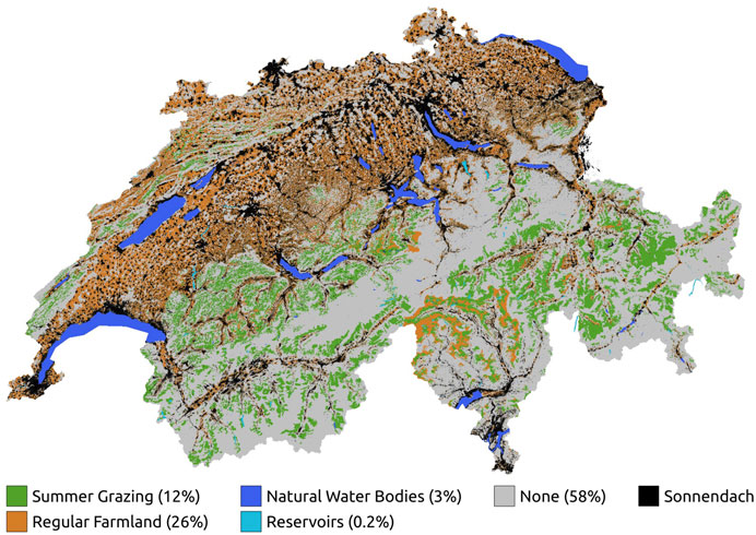
FIGURE 1. Overview of the four landuse classes used for aggregating the different radiation maps plus the rooftop data “Sonnendach.”

2.3.1 Agricultural land

Agricultural land makes up a large part of the total surface area of Switzerland and thus holds a high potential for solar power production.

Depending on the specific type of agricultural land, different types of solar projects are feasible. For this reason, we further subdivide agricultural farmland into two categories:

• Permanent farm lands: Productive farm land of different cultivation types (meadow, pastures, vines, crop). In this category, solar panels are colocated with crops and farming infrastructure. The term “agri-PV” is often used to describe such solar projects and are quite different in their design parameters as compared to standard utility-scale solar projects. Surface area: 10,864 km².

• Summer grazing lands: Agricultural land which serves as grazing areas for livestock in the summer months, typically (but not exclusively) in alpine areas. On such lands, while there is more flexibility in terms of solar project design, an important requirement for the design is to minimize impedance to animal movements. Surface area: 5,060 km²

The geospatial data for agricultural land used for segmentation was obtained from the cantons through the central service geodienste.ch in the form of GeoPackages and Shapefiles. Due to variations in data release practices among the cantons on this platform, separate datasets were acquired. These datasets were queried to differentiate between “Permanent farm lands” and “Summer grazing lands,” requiring distinct SQL queries to achieve the same semantic result. Subsequently, each subset was transformed into boolean rasters, aligned with the radiation maps explained in the previous section, with a resolution of 25 × 25 m. To exclude forested areas, the SwissTLM3D Landcover dataset by the Federal Office of Topography (swisstopo) was utilized to overwrite any values corresponding to forested areas with NoData. By multiplying these rasters with the radiation maps, new rasters were generated, from which area and mean radiation values could be derived.

2.3.2 Water bodies

Solar projects on stagnant water bodies belong to a niche named “Floating-PV” in the industry. While designing projects on water bodies, the hydrological dynamic must be taken into consideration. Water bodies used for hydroelectrical power production have significant fluctuations in water levels, whereas natural water bodies are more stable. These fluctuations impose critical boundary conditions for solar project design. Furthermore, many of the artificial reservoirs are located high in the Alps and freeze over during the winter months. The freezing of the surface imposes additional constraints on the design. For this reason, we differentiate between two types of water bodies in our analysis:

• Reservoirs Water bodies in proximity to dam structures (these dam structures are also part of the SwissTLM3D dataset). These water bodies are assumed to be utilized for hydroelectric power production. Surface area: 79.9 km²

• Natural water bodies: Water bodies which are not in proximity to dam structures. These water bodies are assumed to be naturally occurring lakes. Surface area: 1,347 km²

The geospatial data for this segmentation is provided by swisstopo in the landscape model SwissTLM3D (“TLMBodenbedeckung—Stehende Gewässer” and “TLMStaubaute”). This data was obtained in the form of vector data, provided as Shapefiles. The water bodies data was initially queried to select objects with a surface area greater than 1 ha. Subsequently, the water bodies were categorized as either “Reservoirs” or “Natural water bodies” based on whether they intersected a dam structure or not. These vector datasets were then converted to boolean rasters with a resolution of 25 × 25 m, matching the radiation maps. In order to exclude sections of large lakes that extend beyond Switzerland’s national boundaries (Lake Geneva, Bodensee, Lago Maggiore), all values outside the national border delineated by swisstopo TLMLandesgebiet were assigned as NoData. And as with the agricultural data, multiplying these modified rasters with the radiation maps, created new rasters, from which area and mean radiation values could be derived.

2.4 Rooftops

Urban areas with extensive built-surface in the form of rooftops have long been considered the ideal surface for large-scale deployment of solar PV assets due to ease of access and installation and close proximity to energy demand. Based on the 3D buildings dataset from swissopo (swissBUILDINGS3D) and the weather data from the Federal Office of Meteorology and Climatology (MeteoSwiss), the “Sonnendach” dataset provided by the Swiss Federal Office of Energy (SFOE) describes the potential energy production for each rooftop in Switzerland (see Figure 1. This study sums up the entire production potential of all roofs of Switzerland, including the roofs that are tilted toward the north. There are many different ways of computing the most suited, i.e., the most productive subset of all these roofs. For example, excluding north-oriented roofs or north-oriented roofs that are steeper than a certain angle … or/and excluding sheds. The fact that there are so many options swayed us toward simply looking at the full potential. Several other studies have already reasoned and assessed the various subset of feasible rooftop areas and we will compare our results with theirs in the results section.

The data was acquired from sonnendach.ch in the form of vector data in the GeoPackage format. Since the dataset already contains surface area and potential yield for each rooftop, no processing was necessary. Swiss law requires solar panels to be flush with the roof, it is thus not possible to optimise their tilt for either annual total or winter production. This constraint is reflected in Section 3, where roof-top potential is limited to 2 bars and not four as for agricultural and water surfaces, where the tilt angle can be freely chosen. The total surface area of all rooftops is 664 km².

3 Results and discussion

We begin the analysis by first discussing the solar-yield maps and then calculating the different optimization results mentioned at the end of Section 2.2. Next, the optimized yield calculations are segmented geospatially and the yields for each sub-landuse category are compared with each other and with rooftop seasonal potential.

3.1 Solar yield maps

The baseline for solar-energy yields is taken as the yield produced by 20-degree tilted PV panels. This value was chosen for two reasons. It is the closest to the average rooftop angle within our list of computed PV geometries and secondly, it is considered roughly as the optimal angle for mid-latitudes. The annual and winter production maps for the baseline solar-yield calculation are shown in Figures 2A, B. The mean, maximum and minimum values of the annual baseline yield potential are 277.82, 418.12, and 29.95 kWh/m² respectively. The large spread in yield potential is directly linked to the topographical complexity in the landscape. This can be seen in the maps where the heterogeneity of the yield values is maximal in the alpine region. On the other hand, the central plateau diagonally cutting across the country has relatively homogeneous values.

FIGURE 2

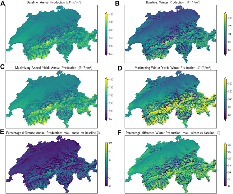
FIGURE 2. (A,B) Baseline production values for annual and winter production respectively. The maps are based on 25 m resolution raster data computed according to Section 2.1. The baseline is taken as production from a 20° tilt PV panel. (C) Annual production for the maximum annual yield scenario, (D) Winter production for the maximum winter yield scenario, (E) Percentage difference between (C,A) subplots, (F) Percentage difference between (D,B) subplots.

Figures 2C, D show the annual and winter yield values from an optimization process where the geometry of each pixel is chosen such that the annual yield and the winter yield are maximized respectively. In qualitatively comparing sub-figures (c) with (a) and (d) with (b), it can be noted that the difference of the optimization process is more prominent in the winter optimization while the corresponding differences in the annual total yield are much less pronounced. Figures 2E, F quantify these differences. The annual optimized scenario has on average 1.75% more production. This difference jumps when looking at the winter-only production values where a much bigger increase of 16.5% is found with the maximum difference of 31%. Thus, it is clear that if winter energy production is to be boosted, changing the tilt geometry from 20° is imperative.

The optimal tilt angles for maximizing annual and winter production are shown in Figures 3A, B respectively. For maximizing annual production, the optimal angle is found to be 30° for most of the country with higher angles found in the alpine areas. To maximize winter production, the optimal tilt changes to 60° in most parts of the country with the upper alpine stretches showing optimal angles of 70° as well. Thus, the choice between maximizing annual and winter productions implies a significant change in the design of solar projects.

FIGURE 3

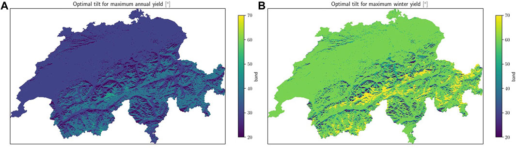
FIGURE 3. (A) Tilt angles for maximizing annual production at 25 m resolution. (B) Tilt angles for maximizing winter production at 25 m resolution.

3.2 Aggregated production potential per landcover type

Figures 4, 5 compare the production potential of the three major landcover types considered in this study. The first comparison is in absolute terms (Figure 4) and shows the total amount of energy that could be produced in each category. Following in Figure 5, you see a direct comparison of the production per m² of PV panel surface. The yield is split into summer (April-September) and winter (October-March) season comparing panels tilt maximised for annual total production and for winter production respectively. The rooftop category has only 2 bars since the panel tilt is dictated by the inclination of the roof and does not allow for optimization.

FIGURE 4

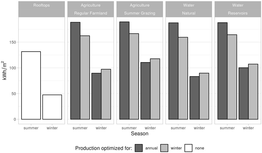
FIGURE 4. Aggregated production potential for all landuse classes. Four bars per class, showing total energy yield subset into winter and summer season, each for two different tilt optimizations (annual max and winter max). Rooftop installations cannot be optimized, thus only 2 bars. Small values ($<$50 TWh) are labelled above the bar.

FIGURE 5

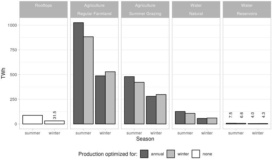
FIGURE 5. Production potential for all landuse classes. Four bars per class, showing energy yield per m² subset into winter and summer season, each for two different tilt optimizations (annual max and winter max). Rooftop installations cannot be optimized, thus only 2 bars.

Corresponding to the respective surface areas of the different landcover types (Permanent farm land: 10,864 km², Summer grazing land: 5,060 km², Natural water: 1,347 km², Rooftops: 664 km², Reservoirs: 80 km²), we see a clear dominance of production potential in the agricultural zones. Regular farmland covers a quarter of the entire country and has a total production potential of about 1,500 TWh/a. For reference: the Swiss electricity demand in 2035 is estimated to be around 60 TWh/a. Summer grazing land could produce around 750 TWh/a, natural standing water around 200 TWh/a, rooftops around 120 TWh/a and reservoirs around 10 TWh/a. In all cases, optimizing the tilt for winter production will generate a slightly lower yield throughout the year than optimization for the annual total. But it increases the much-needed winter electricity production. Of course, we need to keep in mind that only a small fraction of the total area can be dedicated to solar energy production. Different approaches to finding the subset of area, where PV installations would be feasible have been published in the past. For rooftops reductions to between 15 TWh/a and 60 TWh/a have been suggested (Cattin et al., 2012; Bartlett et al., 2018). The ZHAW found a feasible potential energy yield of 120 TWh/a for agricultural zones (Jaeger et al., 2022). A whitepaper published by Energiezukunft Schweiz AG (Wanner et al., 2022) suggests a reasonable coverage of 5 percent of all water surfaces, with an associated production potential of 15 TWh/a. The sensibly exploitable yield of artificial reservoir is estimated to be around 350 to 450 GWh/a (Maddalena et al., 2022). Given the wide range of what is considered feasible or reasonable, it is also important to look at the amount of electricity that could be produced per PV surface area installed in the different classes. Figure 5 shows a direct comparison between the different classes in kWh/m². Here, it becomes very clear that rooftops are not the optimal place for efficient electricity production. Especially in winter, the energy yield is far behind the other categories; at about half of the production in agricultural zone and water surfaces (less than 50 kWh/m² vs. around 100 kWh/m²). In these latter zones, the winter energy ranks with average elevation of the landcover class. Summer grazing land which is to be found primarily around the alpine slopes in the southern part of the country has the highest winter potential, closely followed by artificial reservoir which are also higher up in the alpine valleys. Lowest winter energy yields are calculated for the natural lakes which are largely situated in the lowest parts of the country. The summer energy potential is very similar for all agricultural and water surfaces, but again the rooftops provide much less; their yield is about 25 percent lower. In realistic future installations the difference would be even higher since most ground-mounted or floating installations would be built with bifacial panels and not—as assumed in our study - with monofacial panels. For rooftops this option only exists for flat roofs, which represent about a quarter of the roof area (Anderegg et al., 2022).

4 Conclusion

In this article novel surface radiation maps and associated solar-yield potentials were presented for the territory of Switzerland. The novelty of the maps lies in the extremely high spatial resolution of 25 m. This resolution allows for proper representation of the solar yield potential in areas with high topographic complexity, a characteristic feature of large areas of Switzerland.

The solar yield calculations were performed for multiple tilt angles and two separate scenarios were derived: maximum annual production and maximum winter production. The optimal tilt angles for these scenarios are different and were presented. For most of the Swiss territory, the optimal angles are 30° and 60° for maximum annual and winter production.

An important input for policymakers is to know yield potentials for landuse classes so that suitable policies can be drafted for promoting solar PV. Towards this goal, the seasonal (summer and winter) yield potentials for the scenarios described above were segmented into four sub-groups: Permanent farm land, summer grazing areas, natural water bodies and reserviors. Apart from the policy question, the choice of these sub-groups was motivated by the fact that PV projects on each sub-group occupy different design and installation niches such as “agri-PV” and “floating-PV”.

The yields in the subgroups were analyzed in two ways, total yield in each sub-group—a question of interest to policymakers and yield efficiency in terms of yield per square meter of PV surface area—a crucial number for financial modelling of PV projects. For reference, the rooftop yields were treated as a baseline. In terms of total yield potential, agricultural regions dominate as expected owing to large surface areas dedicated to agricultural activities. The summer grazing regions, which overall have the second largest total yield potential incidentally have the highest efficiency, particularly in the winter. The second highest yield efficiency is found in the water reservoirs. All the four sub-groups analyzed have higher efficiencies than rooftop yield. This is not a surprise as there is no room for optimization through tilt correction on rooftop installations.

While this work only performed a high-level geospatial segmentation, the public release of high-resolution yield maps generated in this work enables a new generation of geospatial analyses where the depth and complexity of the analyses are adequately matched with the input datasets.

Data availability statement

The datasets presented in this study can be found in online repositories. The names of the repository/repositories and accession number(s) can be found below: https://doi.org/10.5281/zenodo.8296864.

Author contributions

NR: Conceptualization, Data curation, Formal Analysis, Methodology, Software, Visualization, Writing–original draft, Writing–review and editing. AK: Conceptualization, Funding acquisition, Project administration, Writing–original draft, Writing–review and editing. VS: Conceptualization, Data curation, Formal Analysis, Methodology, Resources, Software, Supervision, Visualization, Writing–original draft, Writing–review and editing.

Funding

The research published in this report was carried out with the support of the Swiss Federal Office of Energy SFOE as part of the SWEET EDGE project (SI/502269-01).

Acknowledgments

The authors would like to thank Anja Schilling, Isabelle Derivaz-Rabii and Flora Dreyer for their valuable and enthusiastic support with all logistic and administrative tasks during the research and writing phase of this study. The work would not have been possible without the tools made available by the open-source software community.

Conflict of interest

Authors AK and VS were employed by SUNWELL SARL.

The remaining author declares that the research was conducted in the absence of any commercial or financial relationships that could be construed as a potential conflict of interest.

Publisher’s note

All claims expressed in this article are solely those of the authors and do not necessarily represent those of their affiliated organizations, or those of the publisher, the editors and the reviewers. Any product that may be evaluated in this article, or claim that may be made by its manufacturer, is not guaranteed or endorsed by the publisher.

References

Anderegg, D., Strebel, S., and Rohrer, J. (2022). Photovoltaik Potenzial auf Dachflächen in der Schweiz. Ittigen, Switzerland: Energie Schweiz. doi:10.21256/zhaw-2425

CrossRef Full Text | Google Scholar

Bartlett, S., Dujardin, A., Kruyt, B., Manso, P., and Lehning, M. (2018). Charting the course: A possible route to a fully renewable swiss power system. Energy 163, 942–955. doi:10.1016/j.energy.2018.08.018

CrossRef Full Text | Google Scholar

Bucher, C., Huegi, M., Wyrsch, N., and Ballif, C. (2023). Report pv-potential ch (currently under review).

Google Scholar

Buffat, R., Grassi, S., and Raubal, M. (2017). A scalable method for estimating rooftop solar irradiation potential over large regions. Appl. Energy 216, 389–401. doi:10.1016/j.apenergy.2018.02.008

CrossRef Full Text | Google Scholar

Cattin, R., Schaffner, B., Humar-Maegli, T., Albrecht-Widler, S., Remund, J., Engel, J., et al. (2012). Energiestrategie 2050 – Berechnung der Energiepotenziale für Wind- und Sonnenenergie. Bern, Switzerland: Meteotest.

Google Scholar

Dozier, J., and Frew, J. (1990). Rapid calculation of terrain parameters for radiation modeling from digital elevation data. IEEE Trans. Geoscience Remote Sens. 28, 963–969. doi:10.1109/36.58986

CrossRef Full Text | Google Scholar

Egli, F., Haelg, L., Schreiber, M., and Schwarz, M. (2022). Alpenstrom jetzt! (AlpEnForce).

Google Scholar

Energiegesetz (2022). Dringliche Massnahmen zur kurzfristigen Bereitstellung einer sicheren Stromversorgung im Winter. https://www.fedlex.admin.ch/eli/oc/2022/543/de (Accessed June 1, 2023).

Google Scholar

Gutschner, M. (2006). Potenzial des Solarstroms in der Gemeinde. St. Ursen, Switzerland: NET Nowak Energie Technologie AG.

Google Scholar

Gutschner, S., Nowak Ruoss, D., Toggweiler, P., and Schoen, T. (2002). Potential for building integrated photovoltaics. Paris, France: International Energy Agency.

Google Scholar

Haelg, L., Schmidt, T. S., and Sewerin, S. (2022). The design of the Swiss feed-in tariff. Cham, Germany: Springer International Publishing, 93–113. doi:10.1007/978-3-030-80787-0_5

CrossRef Full Text | Google Scholar

Hitachi, , and Siemens, (2023). Personal communication.

Google Scholar

International Energy Agency (2022). World energy outlook. https://www.iea.org/reports/world-energy-outlook-2022 (Accessed May 1, 2023).

Google Scholar

Iqbal, M. (2012). An introduction to solar radiation. Amsterdam, Netherlands: Elsevier.

Google Scholar

Jaeger, M., Vaccardo, C., Boos, J., Junghardt, J., and Schibli, B. (2022). Machbarkeitsstudie Agri-Photovoltaik in der Schweizer Landwirtschaft. Winterthur, Switzerland: ZHAW Zurich University.

Google Scholar

Kahl, A., Dujardin, J., and Lehning, M. (2018). The bright side of pv production in snow-covered mountains. Proc. Natl. Acad. Sci. U. S. A. 116, 1162–1167. doi:10.1073/pnas.1720808116

PubMed Abstract | CrossRef Full Text | Google Scholar

Maddalena, G., Hohermuth, B., Evers, F., Boess, R., and Kahl, A. (2022). Photovoltaik und Wasserkraftspeicher in der Schweiz—Synergien und Potenzial. Wasser Energ. Luft 3, 153–160.

Google Scholar

Meyer, L., Weber, A.-K., and Remund, J. (March 2023). Das Potenzial der alpinen PV-Anlagen in der Schweiz, (PV-Symposium Kloster Banz, March 2023)

Google Scholar

Moro, N., Sauter, D., Strebel, S., and Rohrer, J. (2021). Das Schweizer Solarstrompotenzial auf Dächern. Winterthur, Switzerland: ZHAW Zurich University.

Google Scholar

Portmann, M., Galvagno-Erny, D., Lorenz, P., and Schacher, D. (2022). Sonnendach.ch: Berechnung von Potenzialen in Gemeinden. Kriens, Switzerland: e4plus AG.

Google Scholar

Remund, J. (2019). Das Schweizer PV-Potenzial basierend auf jedem Gebäude. Bern, Switzerland: Meteotest.

Google Scholar

Remund, J. (2020). Detailanalyse des Solarpotenzials auf Dächern und Fassaden. Bern, Switzerland: Meteotest.

Google Scholar

Remund, J. (2017). Solarpotenzial Schweiz. Solarwärme und PV auf Dächern und Fassaden. Bern, Switzerland: Meteotest.

Google Scholar

Schmetz, J., Pili, P., Tjemkes, S., Just, D., Kerkmann, J., Rota, S., et al. (2002). An introduction to meteosat second generation (msg). Cover Bull. Am. Meteorological Soc. Bull. Am. Meteorological Soc. 83, 977–992. doi:10.1175/1520-0477(2002)083-0977:AITMSG-2.3.CO;2

CrossRef Full Text | Google Scholar

Sharma, V. (2023). Dataset for Geospatial segmentation of high-resolution photovoltaic production maps for Switzerland. Front. Energy. doi:10.5281/zenodo.8296864

CrossRef Full Text | Google Scholar

Sweet Edge (2023). Swiss energy research for the energy transition https://www.sweet-edge.ch/en/home (Accessed May 1, 2023).

Google Scholar

Swiss Federal Office of Energy (SFOE) (2022a). Sonnendach https://www.uvek-gis.admin.ch/BFE/sonnendach/?lang=en (Accessed May 1, 2023).

Google Scholar

Swiss Federal Office of Energy (SFOE) (2022b). Sonnenfassade https://www.uvek-gis.admin.ch/BFE/sonnenfassade/?lang=en (Accessed May 1, 2023).

Google Scholar

Swiss Federal Office of Energy (SFOE) (2020). Swiss energy perspectives 2050+ https://www.bfe.admin.ch/bfe/en/home/policy/energy-perspectives-2050-plus.html (Accessed May 1, 2023).

Google Scholar

Swissgrid (2022). The grid must always be taken into account when installing a solar plant https://www.swissgrid.ch/en/home/newsroom/blog/2023/the-grid-must-always-be-taken-into-account-when-installing-a-solar-plant.html (Accessed June 27, 2023).

Google Scholar

Walch, A. (2022). Spatio-temporal estimation of renewable energy potential in built environments using big data. PhD Thesis. Lausanne, Switzerland: Swiss Federal Institute of Technology Lausanne.

Google Scholar

Walch, C. R. M. N., and Scartezzini, J.-L. (2018). Big data mining for the estimation of hourly rooftop photovoltaic potential and its uncertainty. Appl. Energy 163, 942–955. doi:10.1016/j.apenergy.2019.114404

CrossRef Full Text | Google Scholar

Wanner, A., Grueter, L., and Arnold, M. (2022). Schwimmende Solarkraftwerke auf Schweizer Seen. Basel, Switzerland: Energie Zukunft Schweiz AG.

Google Scholar